An Efficient and Robust Improved A* Algorithm for Path Planning

Abstract

Path planning plays an essential role in mobile robot navigation, and the A* algorithm is one of the best-known path planning algorithms. However, the conventional A* algorithm and the subsequent improved algorithms still have some limitations in terms of robustness and efficiency. These limitations include slow algorithm efficiency, weak robustness, and collisions when robots are traversing. In this paper, we propose an improved A*-based algorithm called EBHSA* algorithm. The EBHSA* algorithm introduces the expansion distance, bidirectional search, heuristic function optimization and smoothing into path planning. The expansion distance extends a certain distance from obstacles to improve path robustness by avoiding collisions. Bidirectional search is a strategy that searches for a path from the start node and from the goal node at the same time. Heuristic function optimization designs a new heuristic function to replace the traditional heuristic function. Smoothing improves path robustness by reducing the number of right-angle turns. Moreover, we carry out simulation tests with the EBHSA* algorithm, and the test results show that the EBHSA* algorithm has excellent performance in terms of robustness and efficiency. In addition, we transplant the EBHSA* algorithm to a robot to verify its effectiveness in the real world.

1. Introduction

Robots have been rapidly developed and widely used in the past decades, especially in typical transportation application scenarios such as airports, ports, warehousing, and logistics. In addition to traditional fixed industrial robots, mobile and humanoid robots have developed the fastest. Autonomous navigation is a basic ability of mobile and humanoid robots. Achieving reliable, safe, and efficient autonomous navigation is a popular research topic in the field of robotics, and it is also a challenge. The four general problems of navigation are perception, localization, motion control, and path planning [1,2,3]. Among these areas, it may be argued that path planning is the most important for navigation processes. Symmetry is widely used in the research of path planning. A* is a path planning algorithm based on graph search, with the search process based on the current node as the center to search for surrounding nodes; this search process is symmetrical. In this manuscript, bidirectional search is one of the optimization strategies of the A* algorithm. Bidirectional search is also a symmetrical path search method. This symmetrical search method can double the efficiency of the algorithm.

Path planning is the determination of a collision-free path in a given environment, which may often be cluttered in the real world [4]. The planned path determines whether a mobile robot can achieve reliable and efficient autonomous navigation. Therefore, path planning plays an essential role in mobile robot navigation. With the widespread application of mobile robots, research on path planning is becoming increasingly popular.

Path planning algorithms can be divided into multiple classifications according to different ways. Graph search-based planners include the Dijkstra algorithm [5], the A-star algorithm (A*) [6], the state lattice algorithm [7] etc. Sampling-based planners include rapidly-exploring random trees (RRT) [8], interpolating curve planners, including lines and circles, clothoid curves, polynomial burves, Bezier curves, spline curves; function optimization planners, including the genetic algorithm [9], swarm particle optimization, etc. Other path planning methods include vision-based path planning, artificial intelligence path planning, etc.

For application scenarios such as warehousing and logistics, path planning in a static environment assumes that the robot perceives the environment and uses local path planning algorithms when the environmental information is not fully grasped. A* is used for shortest path evaluation based on the information regarding the obstacles present in the static environment [10], The shortest path evaluation for the known static environment is a two-level problem which comprises a selection of feasible node pairs and a shortest path evaluation based on the obtained feasible node pairs [11]. Both of the above-mentioned criteria are not available in a dynamic environment, which makes the algorithm inefficient and impractical in dynamic environments. The A* algorithm was chosen because it is among the foundational algorithms used in contemporary real-time path planning solutions in a static environment. Novel research builds on the algorithm to find additional performance and efficiency.

Robustness and efficiency are the two essential factors of the path planning algorithms. Robustness reflects the reliability of the algorithm and is a prerequisite for the safe, stable and fast travel of mobile robots. The path closely fitting obstacles and right-angle turns is among the essential factors that affect the reliability of a mobile robot’s path. Efficiency reflects the speed of the algorithm for path planning and searching, and is one of the basic necessities for high work efficiency in mobile robots. Because robustness and efficiency are also the focus of algorithm improvement, we are also carrying out research along with this thought. This study investigates how to improve the efficiency of the algorithm and enhance the robustness of the algorithm. The research problems are how to reduce the runtime of the algorithm and the number of search nodes, and how to avoid collision and reduce the number of right-angle turns.

To address these two issues, an improvement method named the EBHSA* algorithm is proposed in this paper. It incorporates a series of improvements to the traditional A* algorithm, including the expansion distance, bidirectional search, heuristic function optimization and smoothing. The expansion distance extends a certain distance from obstacles to improve path robustness by avoiding collisions. A bidirectional search is a strategy that searches for a path from the start node and the goal node at the same time. Heuristic function optimization designs a new heuristic function to replace the traditional heuristic function. Smoothing improves path robustness by reducing the number of right-angle turns.

The main contributions of this paper as follows: the EBHSA* algorithm is proposed in this paper, and it includes four optimization strategies in the traditional A* algorithm: expansion distance, bidirectional search, heuristic function optimization and smoothing. Of them, the expansion distance and smoothing are employed to enhance the robustness of the path. The bidirectional search, heuristic function optimization and expansion distance are employed to improve the efficiency of the algorithm. In addition, the EBHSA* algorithm was tested through simulation and compared with other algorithms. The results show that EBHSA* algorithm performs better in terms of robustness and efficiency. In addition to test the effectiveness of the EBHSA* algorithm in actual application scenarios, the EBHSA* algorithm is transplanted to an FS-AIROBOTB mobile robot produced by China HuaQing YuanJian, and tested in the real world.

The rest of this manuscript is organized as follows. A review of the literature on the A* algorithm from the past few years is introduced in Section 2. In Section 3, the basic theory of the A* algorithm and the four optimization methods of the EBHSA* algorithm are introduced. In Section 4, the coarse-grained time complexity analysis of the EBHSA* algorithm is given. The EBHSA* algorithm is tested and compared in Section 5. In Section 6, the EBHSA* algorithm is transplanted to a mobile robot to verify the effectiveness of the algorithm in actual scenarios. Finally, conclusions are given in Section 7.

2. Related Work

The emphasis of path planning is algorithm design. The algorithm processes a geometric model with a certain complexity to generate an appropriate path, and the algorithm verification is completed by means of a robot traveling in the real world. The Dijkstra algorithm [8] and its variants are commonly used in applications such as Google Maps and other traffic routing systems. To overcome Dijkstra’s computational-intensity doing blind searches, A* [12] and its variants are presented as state-of-the-art algorithms for use within static environments [10].

The A* algorithm can plan the shortest path in a map, but it needs to traverse around the path nodes and select the minimum path cost. Therefore, the algorithm performs a large amount of calculation and long calculation time, and the efficiency of the algorithm will decrease with the expansion of the map scale [13]. Due to the characteristics of the graph search algorithm itself, the A* algorithm uses rasterized maps as its map representation method, which makes its path smoothness poor and reliant on too many right-angle turns, resulting in reduced reliability.

Extensive research has been performed on the A* algorithm, mainly focusing on obstacle avoidance, different application scenarios, and algorithm performance optimization in the progress of the A* algorithm. The A* algorithm is a popular graph traversal path planning algorithm. The A* algorithm similar to Dijkstra’s because it is a Dijkstra algorithm modification, in a sense. A* aims to find a shortest path and guides its search towards the shortest path states by a heuristic function. Therefore, the efficiency of the A* algorithm is better than Dijkstra’s. Many works of literature show that the A* algorithm has been widely used in many fields, such as transportation industry [14,15], and with the development of artificial intelligence, the A* algorithm has since been improved, including automated guided vehicle (AGV) [16,17] or unmanned surface vehicle (USV) path planning [18,19] and robot path planning [20,21]. The A* algorithm is simpler and uses less search node, which means less computation than some other path planning algorithms, so it lends itself to more constrained scenarios [22,23].

The A* algorithm needs to search for the shortest path in a map and through a heuristic function for guidance. The heuristic function mainly includes Euclidean distance [24], Manhattan distance [21], diagonal distance [25], and Chebyshev distance. An algorithm is performed and governed by a heuristic function for computation time or run time for the performance of the task.

An A* optimization method with two improvements is proposed to solve the problem of slow search speed and low efficiency of the algorithm [26]. Firstly, the evaluation function is weighted to ensure the reliability of the heuristic function. Secondly, in the rasterized maps, a set of nodes centered on a certain point is constructed. When the set of nodes contains obstacle nodes, this node is defined as an untrusted point and will not be searched. These improvements are used to improve the efficiency of the A* algorithm. However, the optimization method is only one strategy and it increases the calculation amount of the algorithm; moreover, its optimization is not thorough. To improve the efficiency of the A* algorithm, some researchers focused on the storage of traversed nodes and proposed an improved A* storage array method [27]. The storage method is to access the array element by looking up the sequence number when accessing the specified element. This can be completed in one operation, while the traditional A* algorithm needs to traverse multiple nodes to find the specified element. This method only optimizes the storage and access of nodes, and only reduces the calculation amount of the algorithm without improving its path planning. To shorten the calculation time of the A* algorithm, an improved algorithm, called time efficiency A*, is proposed [28]. The proposed algorithm determines the value of the heuristic function before the collision phase, instead of during the initialization phase. Therefore, the algorithm has higher efficiency in calculation time. This optimization method only optimizes the opportunity of determining the value of the heuristic function and does not optimize the heuristic function or decrease the number of search nodes. Therefore, the improvement of efficiency is limited.

Variants of the A* algorithm seem to be invented endlessly. Several A* optimization algorithms are used for a comparison, evaluation, and application scenario selection in [6], including several modifications (Basic Theta*, Phi*) and improvements (RSR, JPS). A hybrid A* algorithm is proposed, improving the traditional A* algorithm when employed in autonomous vehicles. This method can plan the shortest possible path in a hybrid environment for a vehicle.

The A* optimization methods introduced above all only incompletely optimize the efficiency of the algorithm, which means that the efficiency of the algorithm can still be more thoroughly optimized. None of the above algorithms consider optimizing the robustness of the algorithm. Therefore, the improvements and variants of the A* algorithm are still flawed.

A constrained A* approach is proposed for USV in a maritime environment [21], determining the approach path with a USV enclosed by a circular boundary as a safety distance constraint on the generation of optimal waypoints to avoid collision. This means the USV is surrounded by a circuit and reflects the performance of a collision-free approach. The concept of safety distance is also proposed, but the approach with an unmanned surface vehicle enclosed by a circular boundary as a safety distance places a constraint on the generation of optimal waypoints to avoid collision. This means the USV is surrounded by a circuit and not considering the obstacles on the maps.

The path being not smooth enough to dynamically avoid collision is another obvious shortcoming of the traditional A* algorithm. To solve this problem, a global path planning method that perceives the characteristics of the local environment is proposed [29]. This method first uses the A* algorithm to generate the global optimal planning path in a known static map and deletes redundant nodes, and then generates local sequence nodes on the deleted global path to optimize the global path. This method guarantees the performance of the A* algorithm when it is used in a dynamic environment.

Smoothing is one of the most well-known methods to overcome the collision issue. The traditional A* algorithm plans some sharp turns which causes some problems for mobile robots. A smoothing of the A* algorithm is introduced in [20]. The smoothed A* algorithm [19] generates a path and redundant waypoints by using cubic spline interpolation and three path smoothers. Smoothing is one of the most effective methods to reduce right-angle turns and reduce the risk of collision. The A* algorithm is computationally simple relative to other path planning algorithms. With adjustments for vehicle kinematics, steering angle, and other factors, A* and its variants are suitable for AGV [30]. An improved A* path planning algorithm considering economic performance is proposed in [12] to solve the problem of global path planning for autonomous vehicles. New cost functions can be created with respect to equal step sampling, as in the case of Equation (1). The shown cost function includes distance and costs. The above considerations avoid sudden turns and, in this manner, improve the path smoothness [10].

$${f\left(n\right)=k}_1{g\left(n\right)+k}_2{h\left(n\right)+k}_{3}p\left(n\right)$$

(1)

where $k_1$, $k_2$, $k_3$ are weights with a positive value, $g\left(n\right)$ and $h\left(n\right)$ are the same as the base A* function, and $p\left(n\right)$ is the penalty factor based on the turning cost.

A visibility diagram was one of the very first graph-based search algorithms used in path planning in robotics [10,31]. A hybrid A* algorithm with the visibility diagram planning algorithm is proposed in [14] to overcome the issue of high run costs to convergence.

3. The Proposed Methods

In this section, the basic principles of the traditional A* algorithm are introduced, and the deficiencies of the A* algorithm and the reasons for these deficiencies are analyzed. Four optimization methods for the A* algorithm are proposed.

The basic development process of the new algorithm is: the Robot Operating System (ROS) is used as the development platform and we modified the source code. The Dijkstra algorithm contained in ROS is modified and incorporated into the breadth-first search (BFS) method to construct a traditional A* algorithm. On the basis of the A* algorithm, the expansion distance, bidirectional search, new heuristic function, and smoothing are sequentially added, and the EA*, EBA*, EBHA*, and EBHSA* algorithms are developed in sequence. In the following section, we introduce these four optimization strategies and algorithms respectively, and carry out a series of tests on the algorithms.

3.1. Basic Theory of the Traditional A* Algorithm

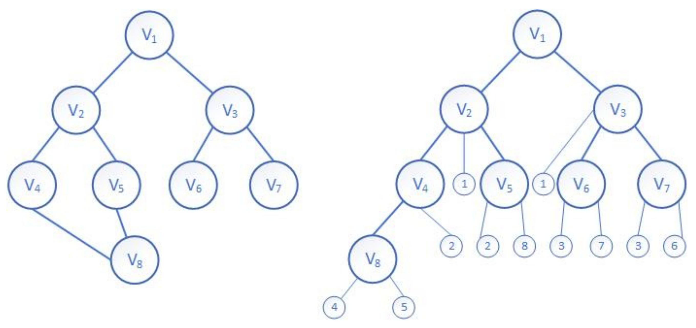
The A* algorithm is a graph search algorithm for path planning, and its search method is based on breadth-first search. In the algorithm, visit to nodes is similar to tree traversal. Only by completing the search of all nodes in this layer can the nodes of the next layer be searched. This may cause blind search and lead to low search efficiency. However, as long as there is a feasible path, it must be able to find and is the optimal path. The process of BFS is shown as Figure 1.

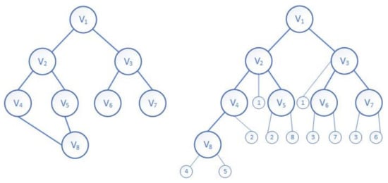
Figure 1. The process of BFS.

The A* algorithm is one of the best-known path planning algorithms and is a classic heuristic search algorithm. The A* algorithm aims to find a path from a start node to a goal node with the smallest cost by searching all possible paths. The heuristic information related to the characteristics of the problem is utilized to guide its performance, so it is superior to blind search algorithms [31]. The A* algorithm consists of an OPEN list, a CLOSED list, and a heuristic function, and it employs the heuristic function to evaluate the distance from an arbitrary node to the goal node on a 2D plane. The A* algorithm is defined as a best-first algorithm because each cell in the configuration space is evaluated by the value:

$$f\left(n\right)=g\left(n\right)+h\left(n\right)$$

(2)

where $g\left(n\right)$ is the cost of the path from the start node to the current node n, $h\left(n\right)$ is the cost of the path from node n to the goal node through the selected sequence of nodes, and $h\left(n\right)$ is the heuristic function of the A* algorithm. $f\left(n\right)$ is denoted as the evaluation function of node n. This sequence ends in the actually evaluated node. Each adjacent node of the actually reached node is evaluated by $f\left(n\right)$. The node with the minimum $f\left(n\right)$ is chosen as the next node in the sequence. The advantage of the A* algorithm is that other distances can be used, modified, or added as standard distances.

3.2. Expansion Distance

The paths obtained by the A* algorithm come close to obstacles. This is unreliable during the movement of a robot. Therefore, a concept is proposed in this paper based on the experience of Euclidean geometry: the expansion distance.

The expansion distance is a certain distance expanding outward along the edge of obstacles before path planning. This is the shortest distance to which the path can approach obstacles. The expansion distance sets a safe buffer area between the path and the obstacles. The nodes of the expansion distance are regarded as obstacle boundaries. In the path planning process, the critical nodes cannot be selected as candidate nodes. The expansion distance can be adjusted according to the size of the robot and the physical environment. A schematic diagram of the expansion distance is shown in Figure 2. The critical node is the node that is in contact with the obstacle, and the expansion node is the node that the algorithm has traversed.

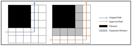
Figure 2. Schematic diagram of the expansion distance.

As the expansion distance is introduced, critical nodes are not traversed during path planning, which is equivalent to reducing the map scale and reducing the total number of nodes that need to be traversed, thereby improving the efficiency of the algorithm.

Because the algorithm does not traverse these critical nodes, the total number of nodes traversed by the algorithm decreases, and the path planning efficiency improves. The main function of the expansion distance is to maintain a certain safe distance between the path and obstacles to ensure the safety of the robot during the traveling process and to facilitate the smooth processing of the path afterward.

3.3. Bidirectional Search Optimization

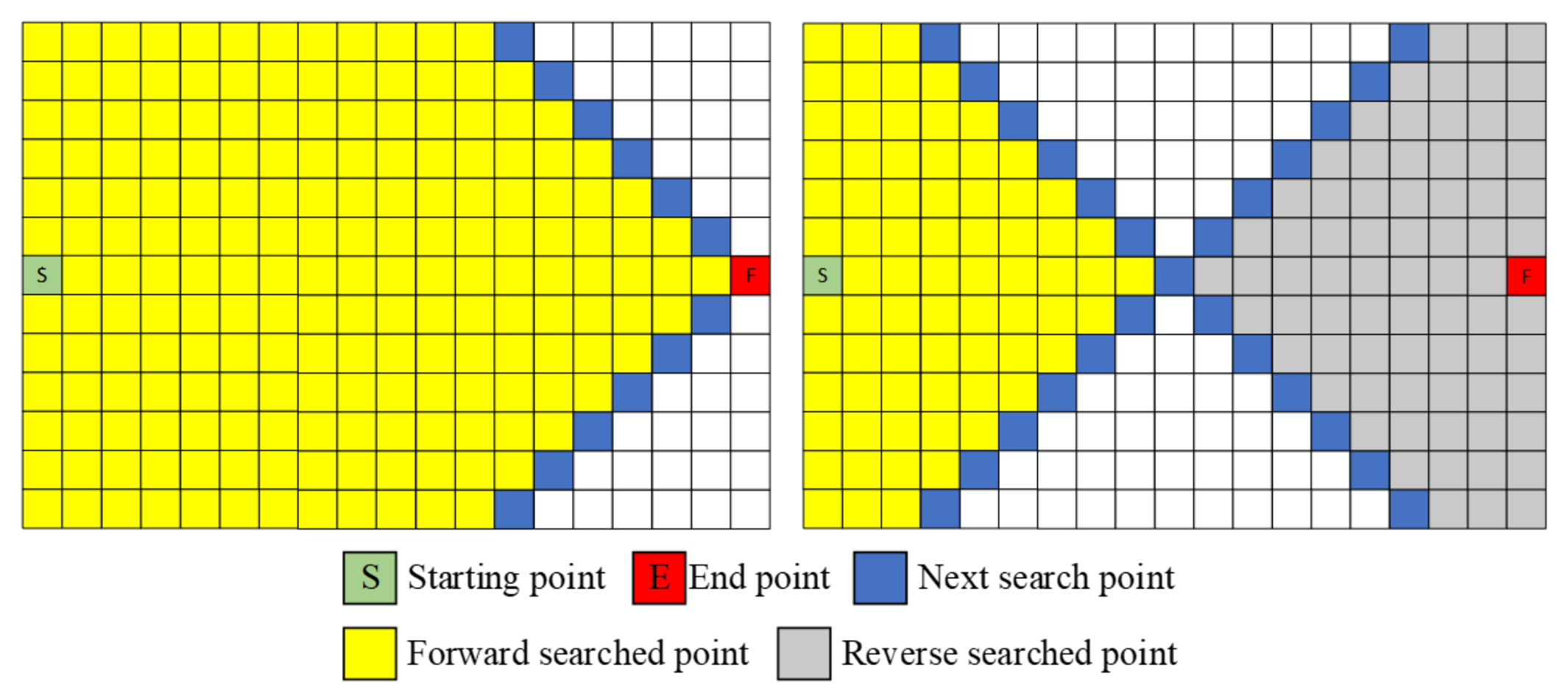
The search process of the traditional A* algorithm is a unidirectional search, finding a path from the start node to the end node. The bidirectional search method is introduced in this paper. The search is conducted from the start node and the end node at the same time. The search process finishes when the forward and reverse search nodes are adjacent during the search process. The positive and negative incomplete paths are spliced together to form a complete collision-free path. A schematic diagram of the search optimization is shown in Figure 3. The left figure is the single search, and the right figure is the bidirectional search.

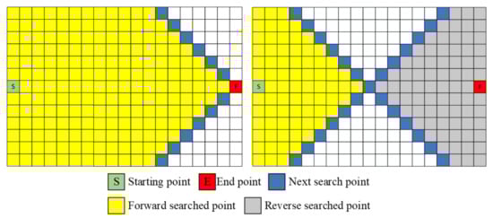
Figure 3. A schematic diagram of search optimization.

The search method introduces this parallel idea and searches from the start node and the goal node at the same time. A function call completes the two searches from the start node and the end node. This reduces the number of function calls and improves the path planning efficiency of the algorithm. In addition, the bidirectional search traverses fewer nodes than the unidirectional search, which further improves the path planning efficiency.

3.4. The Heuristic Function

The heuristic function is the minimum cost evaluation value of the A* algorithm from any node to the goal node and helps to reduce the number of nodes traversed. Therefore, the choice of heuristic function has a direct impact on the efficiency of the algorithm. The heuristic function of the traditional A* algorithm uses the Manhattan distance, and subsequent improvements include the Euclidean distance, diagonal distance and Chebyshev distance. These four heuristic functions are the most widely used functions, and their theories are shown in Formulas (3)–(6).

• Manhattan distance heuristic function

$$h\left(n\right)=/x_a{-x}_{\mathrm{b}}/+/y_a{-y}_b/$$

(3)

2.

Euclidean distance heuristic function

$$h\left(n\right)=\sqrt{{\left(x_a{-x}_b\right)}^2+{\left(y_a{-y}_b\right)}^2}$$

(4)

3.

Diagonal distance heuristic function

$$h\left(n\right)=/x_a{-x}_b/+/y_a{-y}_b/+\left(\sqrt{2}-2\right)\min \left(/x_a{-x}_b/,/y_a{-y}_b/\right)$$

(5)

4.

Chebyshev distance heuristic function

$$h\left(n\right)=\max \left(/x_a{-x}_b/,/y_a{-y}_b/\right)$$

(6)

h(n) is the heuristic function, and $(x_a,y_a)$ are the coordinates of the goal node. $\left(x_b,y_b\right)$ are the coordinates of any node.

The Manhattan distance is mostly used for a 4-direction search. In the case of an 8-direction search, there are too many nodes to traverse. When the Euclidean distance is used, the estimated function value is very similar when the path is close to the goal node, and the node selection may be unclear. When the diagonal distance is used, if there are few obstacles, it is not easy to obtain the shortest path near the goal node. When the Chebyshev distance is used, only the maximum value of the abscissa difference or the ordinate difference is used, and the path always starts from a straight line and then a diagonal, If the search path encounters an obstacle, the shortest path is not obtained.

Based on the analysis of the heuristic function and the experience of repeated experiments, we propose a new heuristic function, as shown in Formula (6).

$$h\left(n\right)=\sqrt{{\left(x_a{-x}_b\right)}^2+ {\left(y_a{-y}_b\right)}^2}+\max \left(/x_a{-x}_b/,/y_a{-y}_b/\right)\times 2$$

(7)

The optimized heuristic function is composed of the Euclidean distance and Chebyshev assignment, according to different weights. This heuristic function not only takes into account the advantages of the Euclidean distance and Chebyshev distance, but also weakens their disadvantages. The first part of the heuristic function ensures that the path is searched along the diagonal direction, and the latter part effectively reduces the number of nodes that are searched around after encountering obstacles in the search process. This advantage is clearly demonstrated in subsequent experiments.

3.5. Smoothing Optimization for Right-Angle Turns

There are three primary disadvantages in the traditional A* algorithm path [19]. The A* algorithm sacrifices the turning cost to find the shortest path length. In addition, a mobile robot needs to decelerate sharply when turning at right-angles, which affects the efficiency and robustness of the algorithm. To overcome these disadvantages, the A* algorithm needs to be improved and smoothed.

In the moving process of the mobile robot, if the turning angle is a right-angle, the turning motion of the mobile robot is broken down into three steps: deceleration, turning on the spot, and movement. This greatly reduces the speed of the mobile robot.

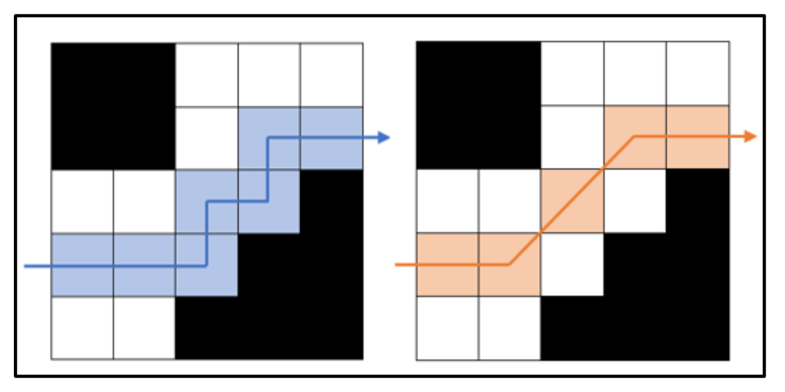
This section mainly optimizes the right-angle turns that are prone to occur during the path planning process. The idea for smoothing right-angle turns is decomposing a 90° turn into multiple small-angle turns to improve the smoothness of the planned path. There are two cases: namely, a single turn, and a continuous turn.

When there are no obstacles on the inside of the corner, the inflection point is deleted, its adjacent two nodes are used as the turning point in the corner, and a right-angle turn is decomposed into two 45° angles, as shown in Figure 4. When there are continuous right-angle turns, the inflection points are removed, and the adjacent nodes are directly connected to convert multiple right-angle turns into a small number of 45° acute-angle turns, as shown in Figure 5. The smoothing optimization of the right-angle turns improves the smoothness of the path, which not only improves the robustness of the algorithm but also improves the overall travel efficiency of the robot.

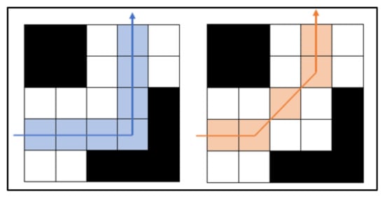
Figure 4. Single right-angle turn smoothing.

Figure 5. Continuous right-angle turns smoothing.

4. EBHSA* Algorithm Time Complexity Analysis

In this section, combining the optimization strategies proposed in Section 3, we conduct a coarse-grained time complexity analysis of the EBHSA* algorithm. This algorithm uses two loops: the inner loop traverses adjacent nodes with the current node as the center, and the node with lowest cost is marked and added to the open table. The outer loop traverses the nodes of the open table until the queue traversal ends. There are several factors that have obvious effects on the time complexity of various path planning algorithms, such as the map scale, starting node and target node location, etc. In general, the time complexity of various algorithms is given by Formula (8):

$$T\in \left[O\left(min\left[m,n\right]\right),O\left(m\ast n\right)\right]$$

(8)

In Formula (8), where $m$ and $n$ are the length and width of the map, respectively. Since a bidirectional search is a strategy that searches in two directions, when the path is solvable, the path formed by each search direction is smaller than the whole path, which reduces the number of nodes added to the open table and reduces the loop frequency. Therefore, the time complexity of the EBHSA* algorithm is less than or equal to half that of the traditional A* algorithm. The pseudocode of the EBHSA* algorithm is shown as Algorithm 1.

Algorithm 1: The pseudocode of the algorithm.

Function: Search(node_i, goal, CLOSE_LIST_i)

Input: Current search node node_i, goal node goal and positive close list CLOSE _LIST_i

Output: A path PATH from Start_i to End_i

Effect: Renew the open list and close list to find the target.

1: Find the surrounding nodes “node(0)”, “node(1)”, “node(2)”, “node(3)” of the node_i

2: for i = 0, i = 3, repeat

3:  if node(i) ∉ CLOSE_LIST_i

4:  heuristic(i) = sqrt((goal_x-node(i)_x)^2 + (goal_y-node(i)_y)^2)

+ max(abs(goal_x-node(i)_x),abs(goal_y-node(i)_y)) × 2

5:  OPEN_LIST_i <- node(i)

6:  else heuristic(i) = ∞

7:  end if

8: end for

For the path planning algorithm, the theoretical time complexity of the algorithm is the size of the entire map, which is O(n²) in this article, but the actual time complexity of the algorithm will vary with the actual map. When there are no obstacles in the map and the algorithm traverses all nodes in the map, the actual time complexity of the algorithm is a theoretical value of O(n²), and the actual complexity must be less than or equal to this value.

5. Simulation Testing

The EBHSA* algorithm was tested using Matlab 2020b, and Matlab 2020b was used for the statistical experiments. All tests were performed on a PC with Windows 10 as OS with I7-1065G7 quad-core CPU and 16GB RAM. A total of 154 maps were created and 181 times simulation tests were performed in this manuscript. In these maps, a total of 5150 × 50 grid maps were generated and tested 60 times, a total of 51,200 × 200 grid maps were generated and tested 60 times, a total of 52,100 × 100 grid maps were generated and tested 61 times, and one map was tested once for the comparison test. All maps and data of the simulation test are shared on GitHub.

Seconds were the used measuring unit for run time. In this simulation, we made several main assumptions to ensure the scientificity and rationality of the test.

• The maps and obstacles of maps are randomly generated. Randomized maps can more accurately verify the universality of the proposed algorithm.
• The size of each obstacle in the map is a 5 × 5 grid, and the number of obstacle center points accounts for about 1.5% of the map scale. A certain number of obstacles can more accurately verify the robustness of the algorithm.
• The firewall, anti-virus software and other software running on the PC were closed during the test to ensure no interference with the execution of the algorithm. We needed to ensure that the algorithm had a stable operating environment during repeated tests, and we found in the test that anti-virus software had a direct impact on the efficiency of the algorithm.
• The running time of the algorithm was used as the only ruler of the efficiency of the algorithm, and its measured unit was seconds.

5.1. Single and Randomized Maps Testing

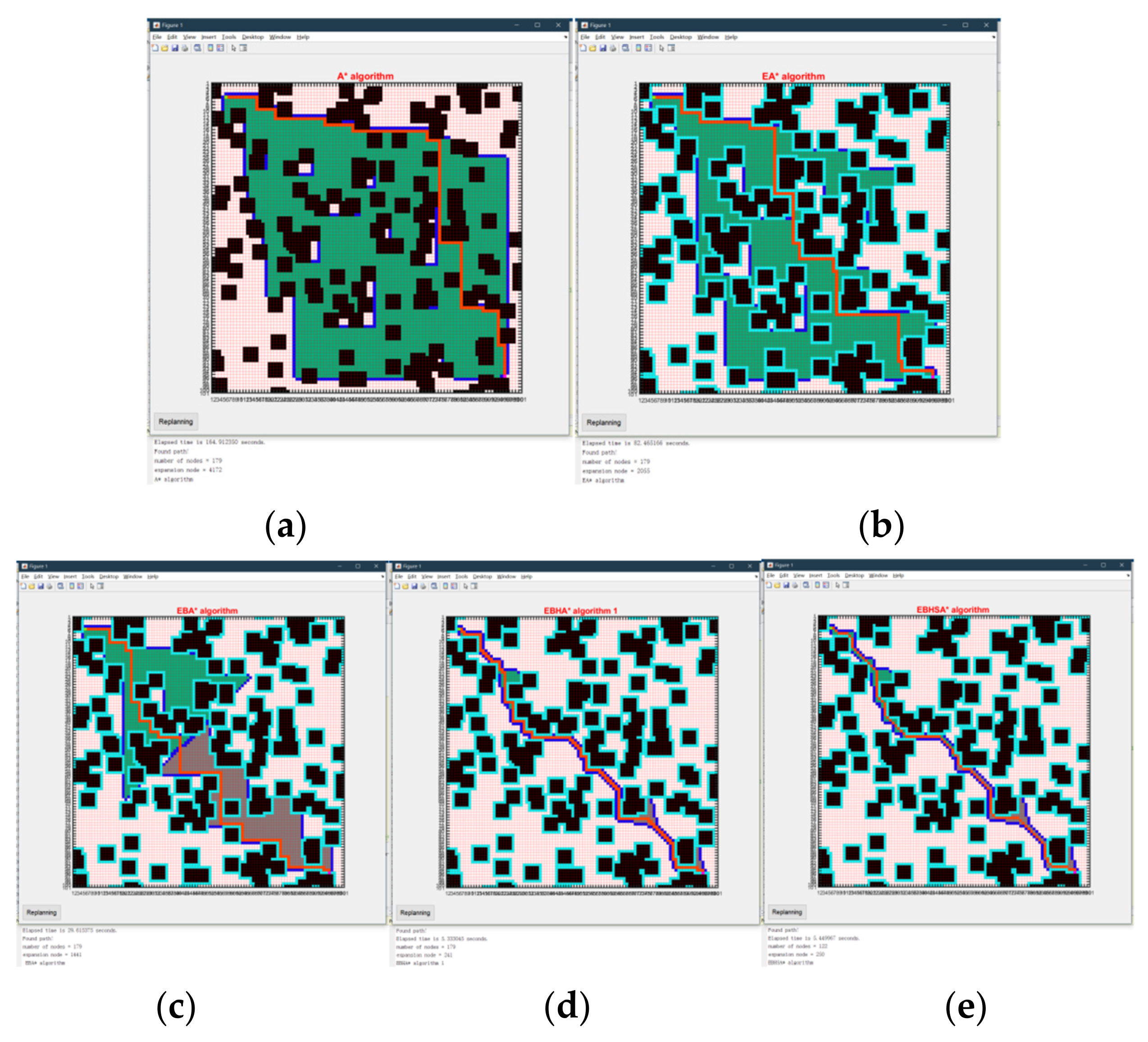
In this section, we simulate and test the five algorithms, traditional A*, A* with expansion distance (EA*), bidirectional EA* (EBA*), EBA* with the heuristic function (EBHA*), and EBHA* with smoothing (EBHSA*). The map scale was 100 × 100 grids in the simulation test. Each grid represents a physical distance of 5 m. The centers of the obstacles were randomly generated. The five algorithms were tested, and the path planning results are shown in Figure 6. The statistical results are shown in Table 1.

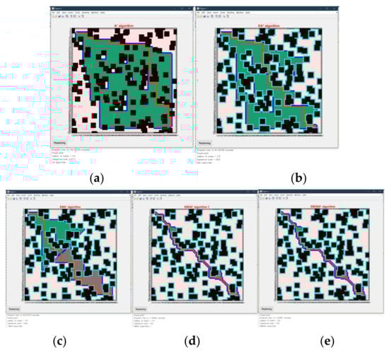
Figure 6. Simulation results of 5 algorithms on a 100 × 100 map scale. (a) A*. (b) EA*. (c) EBA*. (d) EBHA*. (e) EBHSA*.

Table 1. Simulation statistical results of the five algorithms.

Indicators	A*	EA*	EBA*	EBHA*	EBHSA*
Run-time/s	164.912 (100%)	82.465 (50.01%)	29.615 (17.96%)	5.330 (3.23%)	5.450 (3.30%)
Number of nodes	179	179	179	179	122
Number of right-angle turns	19	21	25	29	0
Max turning angle	90°	90°	90°	90°	45°
Number of expansion nodes	4172	2055	1441	241	250
Number of critical nodes	118	0	0	0	7

In Figure 6, the black blocks are randomly generated obstacles, the fluorescent blue blocks around the obstacles are the expansion distances of the obstacles, the green and gray areas are the nodes traversed by the forward and reverse searches respectively, and the red line is the path planned by the EBHSA* algorithm.

Table 1 shows that the run-time represents the total time for the algorithm to complete all path planning actions, such as the search, traverse, expansion, and smoothing. The number of nodes represents the path length. The number of right-angle turns and the maximum turning angle represent the path smoothness. The number of expansion nodes represents the total number of nodes traversed by the algorithm, and the indicator affects the algorithm efficiency. The number of critical nodes indicates the number of nodes adjacent to obstacles in the path.

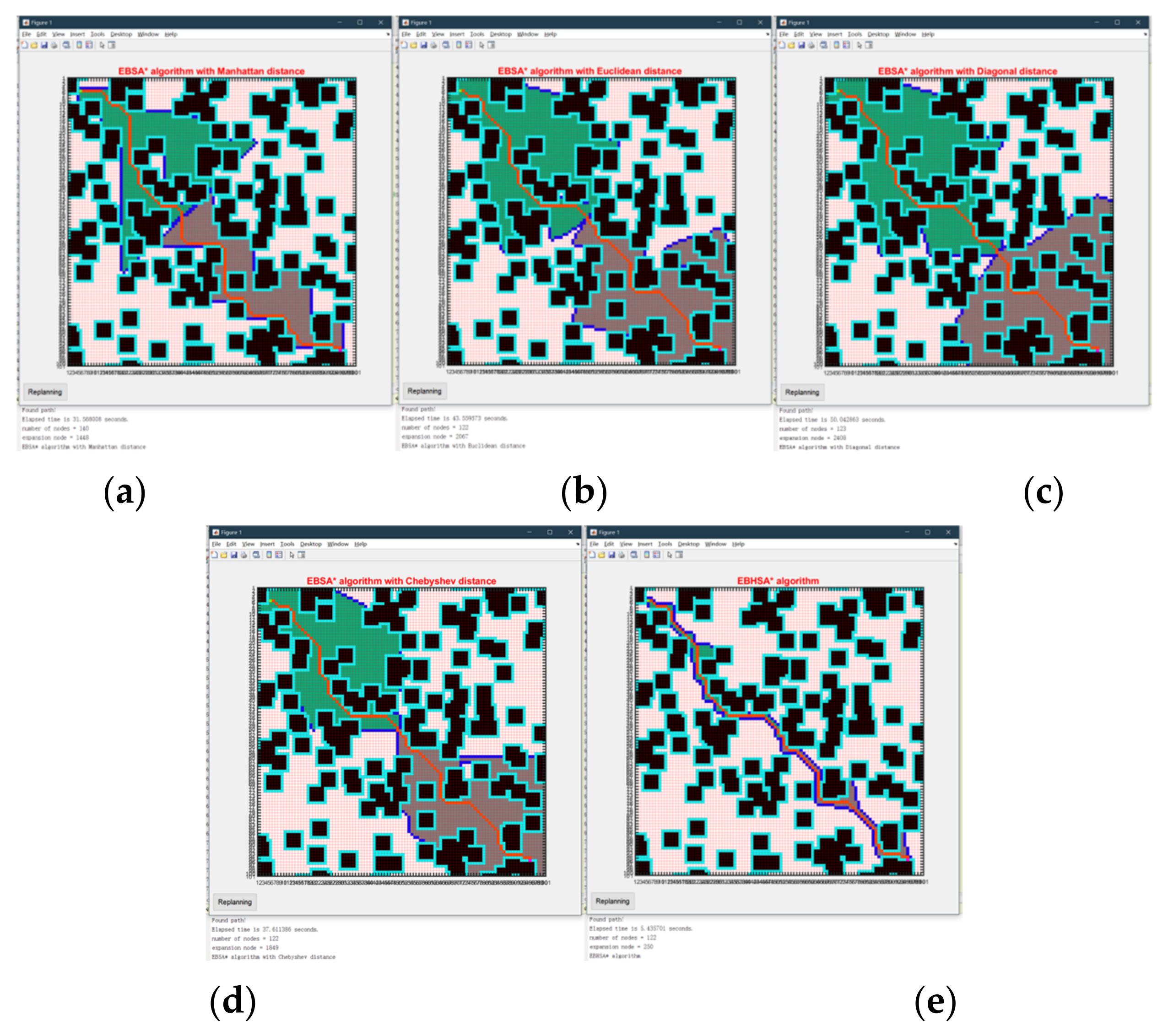
The five heuristic functions were also tested; the results are shown in Figure 7 and the statistical results are shown in Table 2.

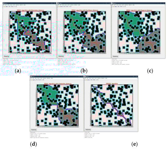
Figure 7. Simulation results of 5 algorithms on a 100 × 100 map scale. (a) Manhattan distance. (b) Euclidean distance. (c) Diagonal distance. (d) Chebyshev distance. (e) EBHSA*.

Table 2. Simulation statistical results of five heuristic functions.

Indicators	EBSA* with Manhattan	EBSA* with Euclidean	EBSA* with Diagonal	EBSA* with Chebyshev	EBHSA*
Runn-time/s	31.568	43.559	50.043	37.611	5.435
Number of nodes	140	122	123	122	122
Number of expansion nodes	1448	2067	2408	1849	250
Number of critical nodes	6	5	8	7	7

The five algorithms and the five heuristic functions were also tested five times on 100 ∗ 100 randomized maps. The test results are shown in Table 3 and Table 4, and all data are averages.

Table 3. Average simulation results of four algorithms on randomized maps.

Indicators	A*	EA*	EBA*	EBHA*	EBHSA*
Run-time/s	219.630 (100%)	155.716 (63.73%)	68.572 (16.80%)	8.080	8.923 (23.35%)
Number of nodes	179	179	180.6	181.4	120.4
Number of expansion nodes	4900.8	3296.2	2749.8	276.6	260.6

Table 4. Average simulation results of five heuristic functions on randomized maps.

Indicators	EBSA* with Manhattan	EBSA* with Euclidean	EBSA* with Diagonal	EBSA* with Chebyshev	EBHSA*
Run-time/s	61.138	83.484	87.521	58.620	8.627
Number of nodes	155.4	122.4	122.2	127.4	123.2
Number of expansion nodes	2697.4	3357.6	3378.4	2450.2	294.8
Number of critical nodes	6	6	7	7	8

The experimental results show that the efficiency of the EBHSA* algorithm was 24.614 times that of the A* algorithm. The run-time of the BA* algorithm was approximately 44.04% of that of the A* algorithm. The results of other indicators in this experiment were also in line with expectations.

To more accurately verify the universality of the algorithm, we repeated the above experiments on maps of different scales, using 50 ∗ 50 grids for small-scale maps, and 200 ∗ 200 grids for large-scale maps. The test data are shown in Table 5, Table 6, Table 7 and Table 8.

Table 5. Simulation statistical results of the five algorithms.

Indicators	A*	EA*	EBA*	EBHA*	EBHSA*
Run-time/s	39.714 (100%)	25.577 (50.01%)	11.429 (17.96%)	1.919 (3.23%)	1.932 (3.30%)
Number of nodes	79	79	79	79	55
Number of right-angle turns	7	11	16	31	0
Max turning angle	90°	90°	90°	90°	45°
Number of expansion nodes	1083	692	593	80	85
Number of critical nodes	35	0	0	0	4

Table 6. Simulation statistical results of five heuristic functions.

Indicators	EBSA* with Manhattan	EBSA* with Euclidean	EBSA* with Diagonal	EBSA* with Chebyshev	EBHSA*
Runn-time/s	11.848	14.958	14.876	12.380	2.036
Number of nodes	61	55	54	54	55
Number of expansion nodes	579	741	736	612	85
Number of critical nodes	4	4	5	5	4

Table 7. Average simulation results of four algorithms on randomized maps.

Indicators	A*	EA*	EBA*	EBHA*	EBHSA*
Run-time/s	51.018 (100%)	39.604 (77.63%)	21.590 (19.52%)	4.395 (8.61)	4.743 (9.29%)
Number of nodes	80.2	79	81.4	82.4	56.4
Number of expansion nodes	1100.6	776	784.2	109.8	122

Table 8. Average simulation results of five heuristic functions on randomized maps.

Indicators	EBSA* with Manhattan	EBSA* with Euclidean	EBSA* with Diagonal	EBSA* with Chebyshev	EBHSA*
Run-time/s	17.742	11.844	13.589	22.005	2.063
Number of nodes	65.4	56.8	55	53.4	54.4
Number of expansion nodes	589.8	817.8	892	766.6	117
Number of critical nodes	3	3	2	3	2

As shown in Table 5, Table 6, Table 7 and Table 8, the test results and statistics results were exactly consistent with the 100 × 100 maps. In addition, after rigorous testing on large-scale maps with 200 × 200 grids, the test and statistics results are also exactly consistent with the 100 × 100 maps.

5.2. Comparison Testing for Other A* Modification

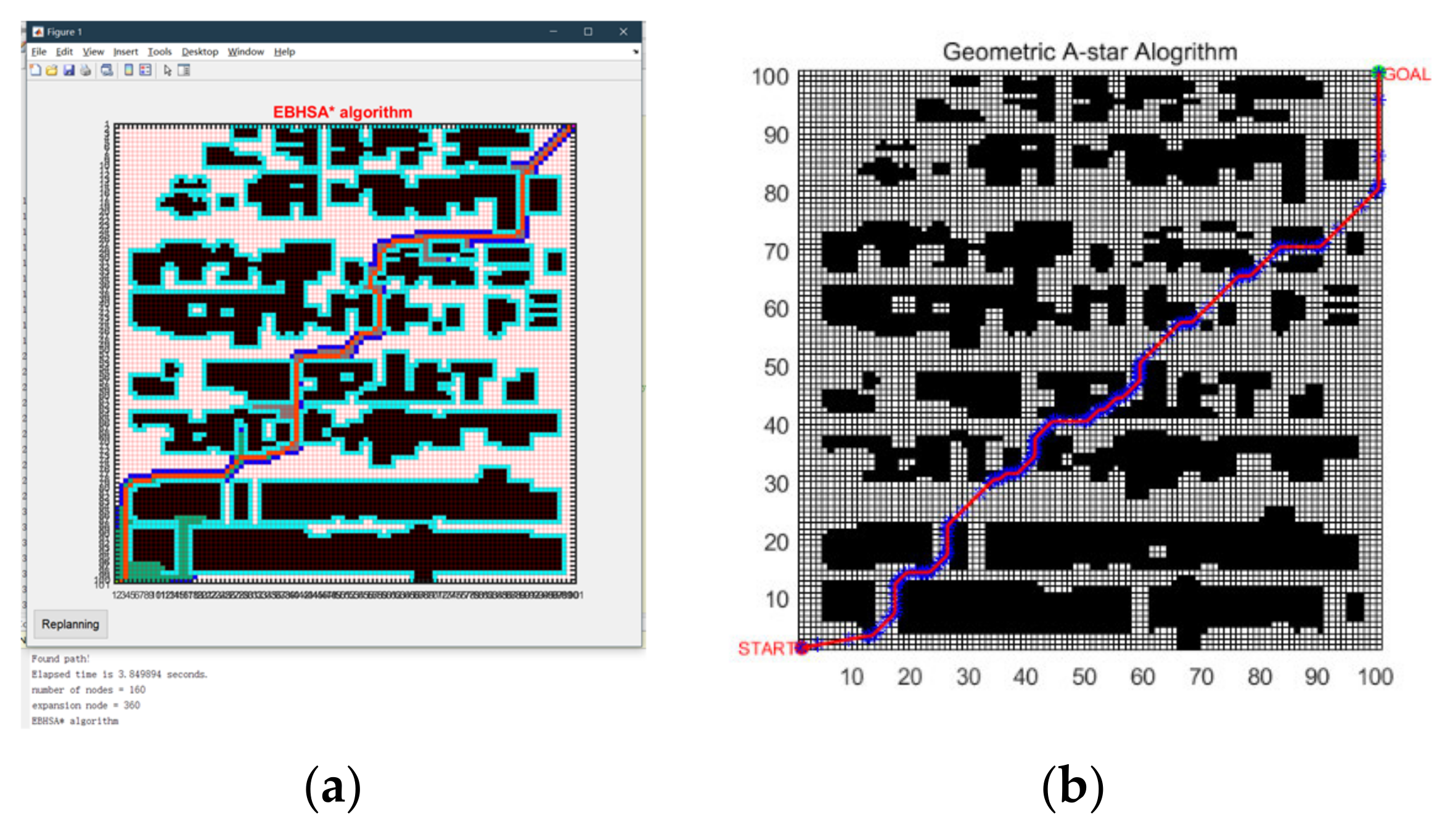
A geometric A* algorithm is proposed in [30] for AGV path planning. The algorithm is also optimized based on the conventional A* algorithm. To compare the efficiency and robustness of EBHSA* and geometric A*, the 100 × 100 scale rasterized map in [30] was reproduced. The path planning result of the EBHSA* algorithm is shown in Figure 8.

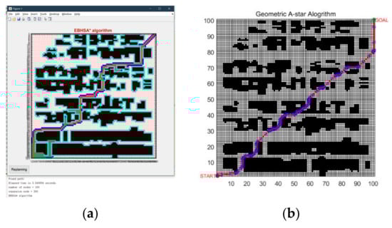
Figure 8. Path planning of the EBHSA* and the Geometric A* algorithm. (a) EBHSA* algorithm. (b) Geometric A* algorithm.

In Table 9, the data of [30] are quoted in the 2nd to 7th columns, and the 8th column is the test results of the EBHSA* algorithm.

Table 9. Algorithm performance comparison.

Indicators	A*	BFS	Dijkstra	Bidirectional A*	DFS	Geometric A*	EBHSA*
Run-time/s	316.334	322.962	316.334	316.334	394.83	295.142	3.850
Number of nodes	131	131	131	131	198	109	160
Number of turns	36	33	27	30	/	27	21
Max turning angle	45°	135°	45°	45°	90°	45°	45°
Number of expansion nodes	2246	5936	6047	1611	198	109	360

Analyzing the data in Table 9 shows that the efficiency of the EBHSA* algorithm was vastly superior to that of Geometric A*. If absolute data are directly used for comparison, it may seem unacceptable because the run-time of the algorithm is affected by many factors, such as the programming language, platform, and computer performance. Therefore, it may be unreasonable to use the absolute time. The A* algorithm was also tested and compared with the Geometric A* algorithm. After careful consideration, the proportional transformation comparison method was used in this comparative experiment. This method is based on the run-time of the A* algorithm in each experiment and calculates the ratio of the two benchmarks: the run-time of the EBHSA* algorithm and the ratio are multiplied to obtain the relative run-time. The relative time was used for comparison with geometric A*. The comparison results are shown in Table 10. The proportional transformation comparison method was also used to compare with the literature [25], and the efficiency of EBHSA* algorithm was 13.83 times.

Table 10. Comparison of the run-times of the geometric A* and the EBHSA* algorithms.

	Conventional A*	Geometric A*	EBHSA*
[30]	316.334	295.142	/
This research	164.912	/	5.450
Ratio	1.918	1	1.918
Relative runtime	/	295.142 *	10.454 *

5.3. Discussion

5.3.1. Efficiency

The experimental results show that the run-time of the EBHSA* algorithm was approximately 3.30% of that of the traditional A* algorithm, which means that the efficiency was 30.26 times that of the A* algorithm. The run-time of the EBA* algorithm was approximately 35.91% of that of the EA* algorithm, and the experimental result was consistent with the time complexity analysis introduced in the previous section. The results of the comparison testing with Geometric A* are shown in Table 5. The efficiency of the EBHSA* algorithm was 28.23 times that of the geometric A* algorithm, an A* modification was 13.83 times faster than suggested in the literature [25].

Analyzing the data in Table 1 shows that the run-time of the EBHSA* algorithm was longer than that of the EBHA* algorithm. This occurred because smoothing was introduced where all nodes of the path needed to be traversed during smoothing and smoothing was performed if a right-angle turn was found. Therefore, EBHSA* effectively enhances the robustness of the path at a small, worthwhile cost.

As shown in Table 2, the efficiency of the EBHSA* algorithm was better than those of the other four heuristic functions in the case of other similar indicators, which means that the proposed heuristic function optimization strategy is significant for path planning.

These data show that EBHSA* algorithm has excellent performance in terms of efficiency; this was one of the original intentions that guided the design of the EBHSA* algorithm.

5.3.2. Robustness

Table 1 shows that the number of path nodes was 31.84% lower than that of the A* algorithm. The maximum turning angle of 45° means that all right-angle turns were smoothed. The number of critical nodes for the A* algorithm was 118, and it was 0 after expansion distance optimization, which means that this strategy effectively enhanced the robustness of the path. In addition, the number of the EBHSA* algorithm critical nodes was higher by seven because critical nodes need to be borrowed when smoothing the corner positions of obstacles. In this case, the right-angle was decomposed into two 45° angles, and the robustness was not significantly reduced. In combination, the number of critical nodes of the EBHSA* algorithm was 94.07% lower, thereby greatly reducing the chance of collisions.

Table 9 shows that the number of turns of the EBHSA* algorithm was the lowest of all the algorithms in the experiment, indicating that its path smoothness was the best. The expansion distance was designed in the EBHSA* algorithm to establish a safe buffer area, and to effectively ensure path robustness. This strategy is especially important in an environment with dense obstacles. The comparison test result is shown in Figure 8a. In Figure 8b, multiple sections of the geometric A* algorithm path are close to obstacles, and the path robustness was greatly threatened. Therefore, it can be concluded that the robustness of the EBHSA* algorithm was better than those other algorithms, including the geometric A* algorithm. This was another goal pursued by the developers of the EBHSA* algorithm.

Since the EBHSA* algorithm does not pursue the shortest path as the target at the beginning of the design, it does not have an advantage in terms of path length. The design idea of the EBHSA* algorithm is to first ensure that the path is reliable, because the cost of collision would be far greater than the performance advantages of other indicators.

The above experiments show that the comprehensive performance of the EBHSA* algorithm is better than that of the other algorithms in the experiments.

6. Effectiveness Test

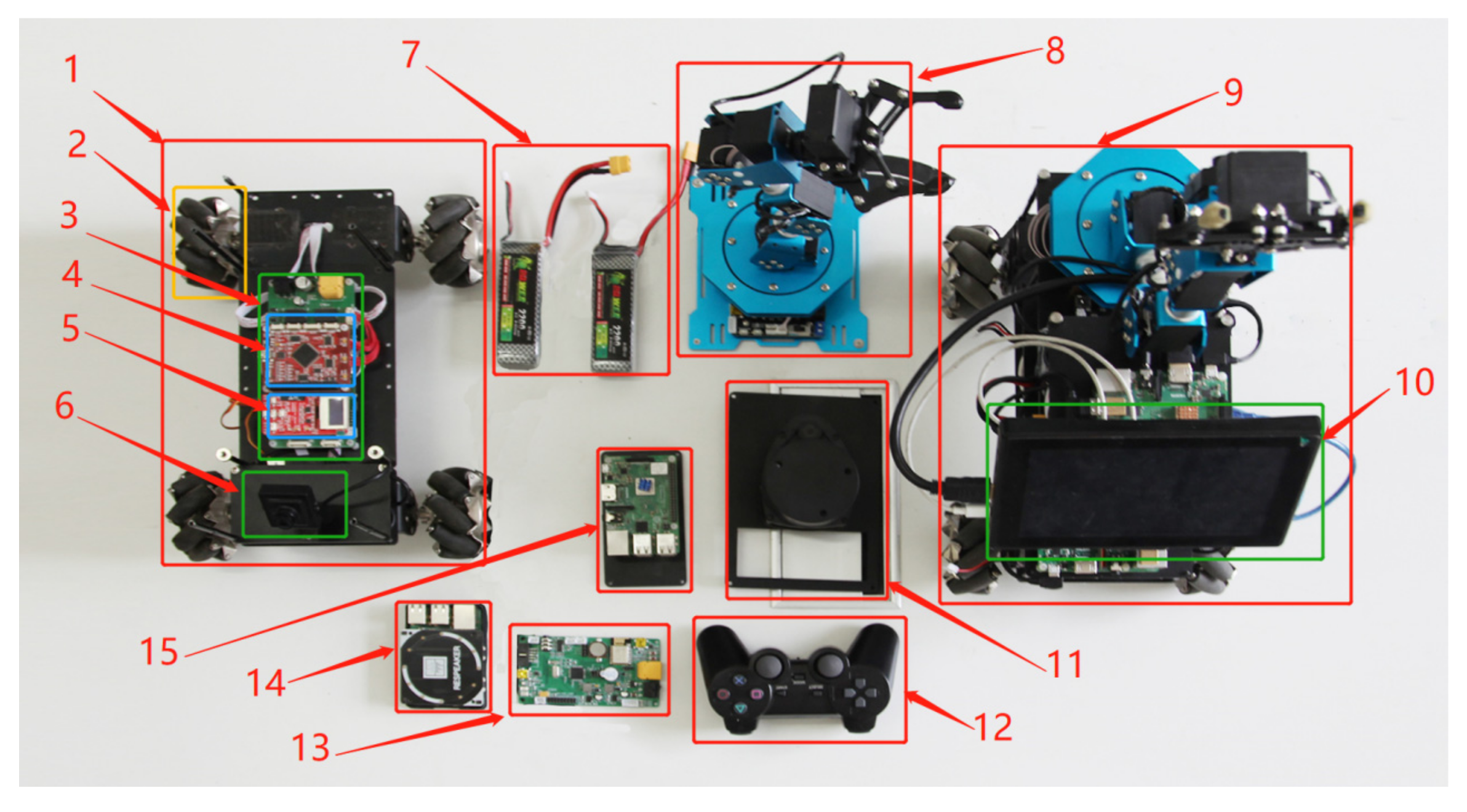
To verify the effectiveness of the EBHSA* algorithm on a real mobile robot platform, the EBHSA* algorithm was transplanted to the FS-AIROBOTB mobile robot hardware platform produced by China HuaQing YuanJian. The algorithm in the open source Robot Operating System (ROS) was rewritten to realize the transplantation of the algorithm. The components are shown in Figure 9, and the parts of each component in Figure 9 are shown in Table 11.

Figure 9. FS-AIROBOTB component diagram.

Table 11. FS-AIROBOTB component serial number comparison table.

Serial Number	Part Name	Serial Number	Part Name
1	ROS omnidirectional vehicle chassis	9	FS_AIROBOTB
2	Mecanum wheel	10	7-inch HDMI display
3	Omnidirectional vehicle drive module	11	360-degree lidar
4	Cortex-M4 chassis core control board	12	Wireless Bluetooth remote control handle
5	FS_Explore sensor board	13	Cortex-M3 robotic arm control board
6	1080P industrial module camera	14	4 array microphones
7	Grep 3S/25C/1300 mA power lithium battery	15	3B+ Raspberry Pi
8	Six degrees of freedom robotic arm

In this experiment, we made several main assumptions to ensure the rationality of the test.

• A real environment is set, and the start point and goal point are set in the scene.
• Since the wheels of the robot are Mecanum wheels with 360-degree steering capability, the initial state of the robot does not require a small space.
• In order to verify the obstacle-free ability of the robot, a certain number of obstacles are set in the real scene.

The effectiveness test is divided into 3 steps: (1) EBHSA* algorithm transplantation, (2) simultaneous localization and mapping (SLAM) test, and (3) a robot autonomous navigation test. The algorithm transplantation involved writing the EBHSA* algorithm into the robot system. The SLAM test built a test map to use the radar on the robot in the real world. The robot autonomous navigation test verified the effectiveness of the algorithm in the real world. To enable other researchers to reproduce our experimental process, we are sharing the source and instructions of this paper on GitHub.

This section mainly introduces the implementation of robot autonomous navigation tests through EBHSA* algorithm transplantation and SLAM map construction to verify the effectiveness of the EBHSA* algorithm in real applications. The corresponding digital map of the real environment constructed through SLAM is shown in Figure 10.

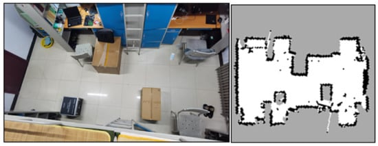
Figure 10. Actual test environment and the map constructed by SLAM.

As shown in Figure 11, the left picture is the rviz interface of the ROS navigation and the right picture is the extracted path.

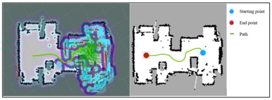
Figure 11. The rviz interface of path planning and extracted path.

In this experiment, we provide a real-world application scenario for the algorithm and carried out basic autonomous navigation tests to verify the effectiveness of the EBHSA* algorithm. The developed algorithm was written into a real mobile robot. The robot could independently plan a reliable and smooth path according to the algorithm and complete the autonomous navigation test from the starting point to the target point. This experiment verifies that the EBHSA* algorithm can be applied to real robots and has the potential to be applied to industrial scenarios.

7. Conclusions

We have presented EBHSA*, an improved A* algorithm for path planning which aims to enhance the algorithm robustness by avoiding collisions and eliminating right-angle turns while improving algorithm efficiency by reducing expansion nodes and run time. Since the A* algorithm was invented for shortest path determination without consideration for robustness, we have presented two strategies for guiding the practice of applying to mobile robots to plan a path for enhancing robustness. The two strategies are expansion distance and smoothing. Moreover, the running time of A* algorithm was also considered to be in need of improvements for efficiency, so we also have presented a set of strategies for improving efficiency. These strategies are bidirectional search, new heuristic function and expansion distance. These strategies should be combined to be used because they have great potential in solving the problems of A* algorithm. We created a scheme for evaluating the performance of EBHSA* algorithm; systematic experiments demonstrated that the EBHSA* algorithm can achieve much higher efficiency than other A* modifications (Geometric A*), while the robustness of EBHSA* algorithm was also effectively enhanced. From Section 5, the EBHSA* has 2925.91% better path planning efficiency, 94.07% fewer critical nodes, and 100% fewer right-angle turns. The practical meaning of this study as to design a path planning algorithm that can be used for mobile robots with excellent efficiency and robustness and has great potential for industrial application in the field of mobile robots.

References

- Zafar, M.N.; Mohanta, J.C. Methodology for path planning and optimization of mobile robots: A review. Procedia Comput. Sci. 2018, 133, 141–152. [Google Scholar] [CrossRef]
- Injarapu, A.S.H.H.V.; Gawre, S.K. A survey of autonomous mobile robot path planning approaches. In Proceedings of the 2017 International Conference on Recent Innovations in Signal Processing and Embedded Systems (RISE), Bhopal, India, 27–29 October 2017; pp. 624–628. [Google Scholar]
- Costa, M.M.; Silva, M.F. A survey on path planning algorithms for mobile robots. In Proceedings of the 2019 IEEE International Conference on Autonomous Robot Systems and Competitions (ICARSC), Porto, Portugal, 24–26 April 2019; pp. 1–7. [Google Scholar]
- Mac, T.; Copot, C.; Tran, D.; Keyser, R. Heuristic approaches in robot path planning: A survey. Robot. Auton. Syst. 2016, 86, 13–28. [Google Scholar] [CrossRef]
- Dijkstra, E. A note on two problems in connexion with graphs. Numer. Math. 1959, 1, 269–271. [Google Scholar] [CrossRef] [Green Version]
- Duchoň, F.; Babinec, A.; Kajan, M.; Beňo, P.; Florek, M.; Fico, T.; Jurišica, L. Path planning with modified a star algorithm for a mobile robot. Procedia Eng. 2014, 96, 59–69. [Google Scholar] [CrossRef] [Green Version]
- Zhang, C.; Chu, D.; Liu, S.; Deng, Z.; Wu, C.; Su, X. Trajectory planning and tracking for autonomous vehicle based on state lattice and model predictive control. IEEE Intell. Transp. Syst. Mag. 2019, 11, 29–40. [Google Scholar] [CrossRef]
- Zhang, L.; Lin, Z.; Wang, J.; He, B. Rapidly-exploring Random Trees multi-robot map exploration under optimization framework. Robot. Auton. Syst. 2020, 131, 103565. [Google Scholar] [CrossRef]
- Tuncer, A.; Yildirim, M. Dynamic path planning of mobile robots with improved genetic algorithm. Comput. Electr. Eng. 2012, 38, 1564–1572. [Google Scholar] [CrossRef]
- Karur, K.; Sharma, N.; Dharmatti, C.; Siegel, J.E. A Survey of Path Planning Algorithms for Mobile Robots. Vehicles 2021, 3, 448–468. [Google Scholar] [CrossRef]
- Dudi, T.; Singhal, R.; Kumar, R. Shortest Path Evaluation with Enhanced Linear Graph and Dijkstra Algorithm. In Proceedings of the 2020 59th Annual Conference of the Society of Instrument and Control Engineers of Japan (SICE), Chiang Mai, Thailand, 23–26 September 2020; pp. 451–456. [Google Scholar]
- Liu, Q.; Zhao, L.; Tan, Z.; Chen, W. Global path planning for autonomous vehicles in off-road environment via an A-star algorithm. Int. J. Veh. Auton. Syst. 2017, 13, 330–339. [Google Scholar] [CrossRef]
- Ziqiang, W.; Xiaoguang, H.; Xiaoxiao, L. Overview of Global Path Planning Algorithms for Mobile Robots. Comput. Sci. 2021, 48, 1–16. [Google Scholar]
- Sedighi, S.; Nguyen, D.V.; Kuhnert, K.D. Guided hybrid A-star path planning algorithm for valet parking applications. In Proceedings of the 2019 5th International Conference on Control, Automation and Robotics (ICCAR), Beijing, China, 19–22 April 2019; pp. 570–575. [Google Scholar]
- Liu, C.; Mao, Q.; Chu, X.; Xie, S. An improved A-star algorithm considering water current, traffic separation and berthing for vessel path planning. Appl. Sci. 2019, 9, 1057. [Google Scholar] [CrossRef] [Green Version]
- Erke, S.; Bin, D.; Yiming, N.; Qi, Z.; Liang, X.; Dawei, Z. An improved A-Star based path planning algorithm for autonomous land vehicles. Int. J. Adv. Robot. Syst. 2020, 17, 172988142096226. [Google Scholar] [CrossRef]
- Zhao, J.; Zhang, Y.; Ma, Z.; Ye, Z. Improvement and verification of A-star algorithm for AGV path planning. Comput. Eng. Appl. 2018, 54, 217–223. [Google Scholar]
- Kim, H.; Park, B.; Myung, H. Curvature path planning with high resolution graph for unmanned surface vehicle. In Robot Intelligence Technology and Applications (RiTA); Springer: Gwangju, Korea, 2013; pp. 147–154. [Google Scholar]
- Song, R.; Liu, Y.; Bucknall, R. Smoothed A* algorithm for practical unmanned surface vehicle path planning. Appl. Ocean Res. 2019, 83, 9–20. [Google Scholar] [CrossRef]
- Gunawan, S.A.; Pratama, G.N.; Cahyadi, A.I.; Winduratna, B.; Yuwono, Y.C.; Wahyunggoro, O. Smoothed A-star Algorithm for Nonholonomic Mobile Robot Path Planning. In Proceedings of the 2019 International Conference on Information and Communications Technology (ICOIACT), Yogyakarta, Indonesia, 24–25 July 2019; pp. 654–658. [Google Scholar]
- Sheikh, T.S.; Afanasyev, I.M. Stereo vision-based optimal path planning with stochastic maps for mobile robot navigation. In International Conference on Intelligent Autonomous Systems; Springer: Cham, Switzerland, 2018; pp. 40–55. [Google Scholar]
- Singh, Y.; Sharma, S.; Sutton, R.; Hatton, D.; Khan, A. A constrained A* approach towards optimal path planning for an unmanned surface vehicle in a maritime environment containing dynamic obstacles and ocean currents. Ocean. Eng. 2018, 169, 187–201. [Google Scholar] [CrossRef] [Green Version]
- Cheng, L.; Liu, C.; Yan, B. Improved hierarchical A-star algorithm for optimal parking path planning of the large parking lot. In Proceedings of the 2014 IEEE International Conference on Information and Automation (ICIA), Hailar, China, 28–30 July 2014; pp. 695–698. [Google Scholar]
- Yang, J.-M.; Tseng, C.-M.; Tseng, P.S. Path planning on satellite images for unmanned surface vehicles. Int. J. Nav. Archit. Ocean Eng. 2015, 7, 87–99. [Google Scholar] [CrossRef] [Green Version]
- Yao, J.; Lin, C.; Xie, X.; Wang, A.; Hung, C.C. Path Planning for Virtual Human Motion Using Improved A* Star Algorithm. In Proceedings of the 2010 Seventh International Conference on Information Technology, New Generations, Las Vegas, NV, USA, 12–14 April 2010; pp. 1154–1158. [Google Scholar]
- Gao, Q.J.; Yu, Y.S.; Hu, D.D. Feasible Path Search and Optimization Based on Improved A* Algorithm. J. Civ. Aviat. Univ. China 2005, 23, 42–45. [Google Scholar]
- Peng, J.; Huang, Y.; Luo, G. Robot Path Planning Based on Improved A* Algorithm. Cybern. Inf. Technol. 2015, 15, 171–180. [Google Scholar] [CrossRef] [Green Version]
- Guruji, A.K.; Agarwal, H.; Parsediya, D.K. Time-Efficient A* Algorithm for Robot Path Planning. Procedia Technol. 2016, 23, 144–149. [Google Scholar] [CrossRef] [Green Version]
- Zhang, X.; Cheng, C.Q.; Hao, X.Y.; Li, J.; Hu, P. A dynamic path planning algorithm for robots with both global and local characteristics. J. Surv. Mapp. Sci. Technol. 2018, 35, 315–320. [Google Scholar]
- Tang, G.; Tang, C.; Claramunt, C.; Hu, X.; Zhou, P. Geometric A-Star Algorithm: An Improved A-Star Algorithm for AGV Path Planning in a Port Environment. IEEE Access 2021, 9, 59196–59210. [Google Scholar] [CrossRef]
- Fu, B.; Chen, L.; Zhou, Y.; Zheng, D.; Wei, Z.; Dai, J.; Pan, H. An improved A* algorithm for the industrial robot path planning with high success rate and short length. Robot. Auto. Syst. 2018, 106, 26–37. [Google Scholar] [CrossRef]
Publisher’s Note: MDPI stays neutral with regard to jurisdictional claims in published maps and institutional affiliations. |
© 2021 by the authors. Licensee MDPI, Basel, Switzerland. This article is an open access article distributed under the terms and conditions of the Creative Commons Attribution (CC BY) license (https://creativecommons.org/licenses/by/4.0/).