An Improvised SIMPLS Estimator Based on MRCD-PCA Weighting Function and Its Application to Real Data

Abstract

Multicollinearity often occurs when two or more predictor variables are correlated, especially for high dimensional data (HDD) where $p>>n$. The statistically inspired modification of the partial least squares (SIMPLS) is a very popular technique for solving a partial least squares regression problem due to its efficiency, speed, and ease of understanding. The execution of SIMPLS is based on the empirical covariance matrix of explanatory variables and response variables. Nevertheless, SIMPLS is very easily affected by outliers. In order to rectify this problem, a robust iteratively reweighted SIMPLS (RWSIMPLS) is introduced. Nonetheless, it is still not very efficient as the algorithm of RWSIMPLS is based on a weighting function that does not specify any method of identification of high leverage points (HLPs), i.e., outlying observations in the X-direction. HLPs have the most detrimental effect on the computed values of various estimates, which results in misleading conclusions about the fitted regression model. Hence, their effects need to be reduced by assigning smaller weights to them. As a solution to this problem, we propose an improvised SIMPLS based on a new weight function obtained from the MRCD-PCA diagnostic method of the identification of HLPs for HDD and name this method MRCD-PCA-RWSIMPLS. A new MRCD-PCA-RWSIMPLS diagnostic plot is also established for classifying observations into four data points, i.e., regular observations, vertical outliers, and good and bad leverage points. The numerical examples and Monte Carlo simulations signify that MRCD-PCA-RWSIMPLS offers substantial improvements over SIMPLS and RWSIMPLS. The proposed diagnostic plot is able to classify observations into correct groups. On the contrary, SIMPLS and RWSIMPLS plots fail to correctly classify observations into correct groups and show masking and swamping effects.

1. Introduction

Multicollinearity occurs when independent variables in the regression model are highly correlated to each other. As a result of multicollinearity, the standard error of the ordinary least squares (OLS) estimate becomes inflated, which weakens the statistical power of the regression model, especially when confronting high dimensional data (HDD). Hence, one may be unable to declare an individual independent variable significant even if it has a strong relationship with the response variable. Moreover, an independent variables’ coefficient may change its signs and renders it more difficult to specify the correct model. Additionally, multicollinearity can cause the correlation matrix of X variables to become singular; thus, OLS fails to produce estimates, and no predictions of the y-variable can be made. These problems become severe when dealing with high dimensional data where $p>>n$. The rapid advancement of computer technology and statistics allows for the generation of data on thousands of variables. Classical multivariate statistical methods are no longer capable of effectively analyzing such high-dimensional data. As a result, Partial Least Squares (PLS) was developed to address this issue, and its applications have gained popularity in a wide variety of natural science fields. For example, PLS is used to quantify genes in genomic and proteomic data. In neuroinformatics, PLS is used to investigate brain function. It is also used in computer science for image recognition and in the engineering industry for process control. PLS was originally designed to solve a problem in chemometrics, but it has since become a standard tool in spectroscopy, magnetic resonance, atomic omission, and chromatography experiments.

Partial Least Squares Regression (PLSR) is introduced with the main aim to build a regression model for multicollinear and high dimensional data with one or several response variables [1]. This method is very popular in chemometrics [2], genomic and proteomic analysis [3], and neural network study [4] and is widely applied in engineering areas. When dealing with one or multivariate responses, the partial least squares regression is commonly referred to as PLS1 or PLS2, respectively. In general, the PLSR method is used to form a relationship between dependent variables and independent variables by constructing new independent explanatory variables called PLS factors, latent variables, or PLS components. The PLS components describe maximum correlations between predictors and response variables. The concept of the PLS method is similar to the Principal Component Regression (PCR) method. As in PCR, a set of uncorrelated components is formed to make a prediction. The major difference between these two procedures is, in the PLS procedure, the PLS components are chosen based on the maximum covariance of $X$ and $Y$ variables while in PCR, the components are chosen with a maximum variance of $X$ variables solely.

There are numerous PLS approaches in the literature, such as NIPALs which was introduced by Wold around 1975 [5]. NIPALS requires deflation of $X$ and $Y$ in order to compute components that are very time consuming for a huge dataset [5]. Lindgren et al. [6] proposed the Kernel Algorithm, and the result is identical to NIPALS but in the Kernel Algorithm, deflation is carried out only for the matrix $X$ in the next computation of components. The latter method also requires much time since the procedure works based on eigen decomposition. The SIMPLS technique was introduced by S. De Jong [7]. In SIMPLS, no deflation of the centered data matrices $X$ and $Y$ is made, but the deflation is carried out based on the covariance matrix, $S=X^{T}Y$. Hoskuldson [8] suggested a method similar to the Kernel Algorithm named the Eigenvector algorithm. The idea is to compute all eigenvectors to the largest eigenvalues, where $k$ is the desired number of PLS components. Orthogonal Projections to Latent Structures (O-PLS) was introduced by Trygg et al. [9] in order to maximize both correlation and covariance between the x and y scores in order to achieve both good prediction and interpretation.

However, it is now evident that PLS is not robust in the sense that its estimate is easily affected by outliers. In regression, outliers can be categorized into vertical outliers, residual outliers, and high leverage points (HLPs) or simply called leverage points [10]. Vertical outliers are outlying observations in the $Y$-space, while residual outliers are observations that have large residuals. HLPs are the outlying observations in the $X$-space. It has the most detrimental effect on the computed values of various estimates, which results in incorrect statistical model development and instills impacts on decision making. Therefore, accurate HLPs detection using reliable methods is vital. In general, classical approaches typically fail to correctly identify outliers in the dataset. As a result, the estimated model will be affected by the masking and swamping problems. ‘Masking’ refers to a situation where outliers are incorrectly declared as inliers, while ‘swamping’ refers to normal observations incorrectly declared as outliers.

Since outliers have an unduly effects on the computed values of various classical estimates, robust methods that are not easily affected by outliers are put forward. Robustness refers to the ability of a method to remain unaffected or less affected by outliers. Several robust alternatives to conventional or classical PLS have been suggested in several literature. The key objective of the robust PLS is to discover contaminated data and reduce their effects by assigning smaller weights to them when estimating a regression model. There are two approaches of robust PLS: down weighting of outliers and robustifying the covariance matrix. For instance, Wakeling et al. [11] used nonrobust initial weights to replace the univariates OLS regression. Cummin et al. [12] proposed iteratively reweighted algorithms, but the weights were not resistant to high leverage points. For the second approach, Gil et al. [13] proposed a method based on constructing robust covariance matrices by using the Stahel–Donoho estimator. However, this method cannot be applied to high-dimensional datasets since it uses a resampling technique by drawing subsets of size p + 2. Hubert and Branden [14] developed robust SIMPLS by constructing a robust covariance matrix using the minimum covariance determinant (MCD) and the idea of projection pursuit to perform on low and high dimensional data. Then in 2005, Serneels et al. [15] proposed partial robust M-regression (PRM) in order to reduce the effect of outliers in $Y$-space and $X$-space of predictor variables. In 2017, Aylin and Agostinelli [16] developed a robust iteratively reweighted SIMPLS (RWSIMPLS) by employing the weight function of Markatou et al. [17]. The weakness of this weight function is that there is no clear discussion on how the effects of outliers or HLPs are reduced since they did not employ any method of identification of outliers or HLPs. It is possible to incorrectly detect and minimize non-outlier observations.

The work of [16] has motivated us to improvise their method, i.e., the robust weighted SIMPLS based on a new robust weighting function. The weight is formulated based on the minimally regularized covariance determinant and principal component analysis (MRCD-PCA) algorithm for the identification of HLPs in HDD. MRCD-PCA is the extension work of MRCD [18], which incorporates the PCA method in the algorithm of MRCD. MRCD-PCA is used for the detection of high leverage points. A simulation study and two real datasets are used to assess the performance of our proposed method compared to SIMPLS and RWSIMPLS. All analyses were performed using R program [16].

The objectives of this study are as follows: (1) to develop a new robust weighted SIMPLS by incorporating a new weight function based on our newly proposed MRCD-PCA algorithm for identifying HLPs; (2) to establish a new algorithm of classifying observations into four categories including regular or good observations, good leverage points (outlying observations in $X$-space), vertical outliers (outlying observations in $Y$-space), and bad leverage points (outlying observations in both $X$-space and $Y$-space); (3) to determine the optimum number of PLS components, denoted as $k$, where $k$ is determined based on the proposed robust root mean squared error prediction, i.e., R-RMSEP; and (4) to evaluate the performance of the proposed method compared to the existing methods, namely SIMPLS and RWSIMPLS. This paper focusses only on PLS1 regression and SIMPLS.

In the next section, we describe the classical SIMPLS algorithm and some existing robust algorithms. In Section 3, we present our proposed MRCD-PCA-RWSIMPLS. In Section 4, we demonstrate the performance of our proposed technique on some simulated data and two real datasets. We compare our method with conventional SIMPLS and the RWSIMPLS methods. We also illustrate our proposed robust diagnostic plots and compute the influence function of real datasets.

2. The SIMPLS Algorithm

The algorithm of SIMPLS maximizes the problem of $t^{T}u=\mathrm{cov}(X_{w,}{Y}_c)\Rightarrow \max$ under the orthogonal constraints of $\Vert u\Vert =\Vert Y_c\Vert =1$ and $\Vert t\Vert =\Vert X_w\Vert =1$. The first SIMPLS component is identical to the NIPALS result or the Kernel algorithm, but the following components are different. In the SIMPLS approach, there is no deflation of the data-centered matrices $X$ and $Y$, but deflation is executed in a covariance matrix or cross-product matrix of $X$ and $Y$, given as $S=X^{T}Y$. Thus, the computation of SIMPLS algorithm is much simpler and less complicated than other PLS algorithms.

2.1. Classical SIMPLS

The multiple linear regression or multivariate regression can be written as follows:

$$y=X\beta +e,$$

(1)

where $X$ is a $n\times p$ matrix, containing $p$ values of explanatory variables at $n$ points. $\beta ={({\beta }_1,{\beta }_2,\dots ,{\beta }_p)}^T$ is a p-dimensional column vector containing regression coefficients, and $e=\left(e_1,e_2,\dots ,e_m\right)$ is $n\times m$ matrix of random errors, and response variable $Y$ is a $n\times m$ matrix, where $m$ is a dimension of response variables at $n$ observations.

In the SIMPLS method, $X$ and $Y$ variables are modeled by linear latent variables based on regression models as in (2) and (3):

$$X=T{P}^T+E_x,$$

(2)

$$Y=U{Q}^T+F_y,$$

(3)

where $X$ is a matrix of predictors with size $n\times p$, and $Y$ is a matrix of response variables with size $n\times m$. $E_x$ and $F_y$ are the error terms, assumed to be independent and identically distributed random normal variables for $X$ and $Y$, respectively. $T$ and $U$ are the score matrices or latent variables of $X$ and $Y$, respectively, and they are formulated as follows:

$$T=XW,$$

(4)

$$U=YC,$$

(5)

for $T=\left(t_1,t_2,t_3\dots ,t_k\right)$ and $U=\left(u_1,u_2,u_3\dots ,u_k\right)$. The $p\times k$ matrix $W$ and the $m\times k$ matrix $C$ are the weight matrices that can be computed by singular value decomposition (SVD). The optimal $X$-weight vector, $w_j$, is the first eigenvector of the eigenvalue problem, and the optimal $Y$-weight vector, $c_j$, is proportional to $Y^{T}X{w}_j$. $w_j$ and $c_j$ are the first left and right singular vectors of the cross-product matrix of $S^j=X^{T}Y$. $k$ is the number of PLS component that is less than or equal to $p$. $P=\left(p_1,p_2,p_3\dots ,p_k\right)$ and $Q=\left(q_1,q_2,q_3\dots ,q_k\right)$ are the $p\times k$ and $m\times k$ orthogonal loading matrices for $X$ and $Y$, respectively.

The fundamental goal of the SIMPLS is to maximize the covariance between the $T$ ($x$-scores) and $U$ ($y$-scores). In conventional SIMPLS, the covariance between vectors t and u is estimated by sample covariance $t^{T}u/\left(n-1\right)$. The constraint of score vectors, $\left|t\right|=\left|u\right|=1$ is needed to solve a problem of maximization. The unique maximization under the constraint of length 1 is given in Equation (6),

$$\mathrm{cov}(t,u)=\mathrm{cov}(X_w,Y_c)=t^{T}u={(X_w)}^T{Y}_c=w^T{X}^T{Y}_c\Rightarrow \max$$

(6)

The first score vectors $t_1$ and $u_1$ are the solutions to the maximization problem for $X$ and $Y$ spaces, respectively. The subsequent score vectors are maximized in the same manner as in Equation (6) with additional constraints that the subsequent score vectors are orthogonal to previous score vectors, i.e., $t_j^T{t}_l=0$ and $u_j^T{u}_l=0$ for $1<j<l<k$. Instead of the original $X$ and $Y$ matrices, orthogonality is provided by finding the subsequent score vectors on the residual matrices. Different algorithms of PLS provide a different method of calculating residual matrices.

Below is the algorithm of the classical SIMPLS approach [5].

Step 1: Compute the centered data matrix, $X$ and $Y$, by subtracting the mean of each column, respectively.

$${\tilde{x}}_{ij}=x_{ij}-mean\left(x_j\right) for i=1,\dots ,n and j=1,\dots ,p$$

(7)

$${\tilde{y}}_{is}=y_i-mean\left(y_s\right) for i=1,\dots ,n and s=1,\dots ,m$$

(8)

Step 2: Based on the centered matrix $X$ and $Y$ in Step 1, determine the initial empirical covariance matrix $S_0=X^{T}Y$.

Step 3: Iterate steps 3 to 9 for $j=1,2,3,\dots ,k$.

If $j=1$, $S_j=S_0$.

If $j>1$, $S_j=S_{j-1}-P_{j-1}{(P_{j-1}^T{P}_{j-1})}^{-1}{P}_{j-1}^T{S}_{j-1}$.

This step accounts for the orthogonal scores on all previous score vectors, as the search is performed in the orthogonal complement of $S_{j-1}$.

Step 4: Perform SVD on $S_j$ and obtain the first left singular vector $w_j$ of $S_j$ where $w_j$ is the dominant eigenvector of $S_j$.

Step 5: $w_j$ is normalized to possess a Euclidean length of 1.

$$w_j=\frac{w_j}{\Vert w_j\Vert }$$

(9)

Step 6: The score matrices $t_j$ are obtained by projecting matrix $X$ on the optimal direction $w_j$, and it can be calculated as follows.

$$t_j={Xw}_j$$

(10)

Step 7: Then, $t_j$ is normalized to possess a Euclidean length of 1.

$$t_j=\frac{t_j}{\Vert t_j\Vert }$$

(11)

Step 8: The loading vector of $X$, $p_j$, is determined by regressing the matrix $X$ on $t_j$.

$$p_j=\frac{X_j^T{t}_j}{t_j^T{t}_j}$$

(12)

Step 9: Next, the loading vector of $Y$, $q_j$ is calculated as follows.

$$q_j=\frac{y_j^T{t}_j}{t_j^T{t}_j}$$

(13)

Note that steps 3 to 9 are iteratively repeated for all extracted $k$ components. Then, the model $y=X\beta +e$ can be estimated by computing the final estimated regression coefficient $\widehat{\beta }$ by using the algorithm above. The parameter estimate $\widehat{\beta }$ is calculated as described in Equation (14):

$$\hat{\beta }=W{(P^{T}W)}^{-1}{Q}^T$$

(14)

where $W$ is the vector of $w_j$, $P$ is the vectors of $p_j$, and $Q$ is the vector of $q_j$. The conventional OLS is applied in step 8 and 9. As already mentioned, the conventional methods such as the OLS method is not robust, i.e., it is easily affected by outlying observations particularly to high leverage points. Subsequently, the empirical covariance matrix is not reliable as it is extremely affected by outlying points. Hence, the SIMPLS algorithm produces non-robust estimates, resulting in inefficient estimates and misleading conclusions about the fitted regression model. These drawbacks have inspired researchers to develop many robust SIMPLS algorithms.

2.2. Robust Iteratively Reweighted SIMPLS (RWSIMPLS)

Aylin and Agostinelli [16] proposed Robust Iteratively Reweighted SIMPLS, which is an improvement of the SIMPLS algorithm where they integrated the weight function suggested by [17] as in Equation (15) in the SIMPLS algorithm in order to reduce the influence of outlying observations in the dataset:

$${\omega }_{r_i}=\omega (r_i(\hat{\beta });m(\cdot ;\hat{\sigma }),{\hat{F}}_n)=\min \left\{1,\frac{{[A(\delta (r_i(\hat{\beta })))+1]}^{+}}{\delta \left(r_i\left(\hat{\beta }\right)\right)+1}\right\}$$

(15)

where $r_i(\hat{\beta })$ is the residual of the estimate $\hat{\beta }$. This weight function depends on the residual, the chosen model distribution density, $m\left(\cdot ;\hat{\sigma }\right)$, and the sample empirical distribution, ${\widehat{F}}_n$. For the RWSIMPLS procedure, the components are extracted by deflating a weighted covariance matrix as described in Equation (16):

$$S^w=X^{w^T}{Y}^w$$

(16)

where $X^w$ and $Y^w$ are the weighted matrices obtained by multiplying each $i^{th}$ row by square root of the following:

$${\omega }_{r_i}=\underset{s}{median}\left({\omega }_{r_{is}}\right) for s=1,\dots ,m and i=1,\dots ,n$$

(17)

where ${\omega }_{r_{is}}$ is the weight of residual corresponding to the $s^{th}$ response, $m$ is a dimension of response variables, and $n$ is the number of observations.

The algorithm of RWSIMPLS can be summarized as follows.

Step 1: Center each of the observation in $X$ and $Y$ matrices by subtracting the median of each column.

$${\tilde{x}}_{ij}=x_{ij}-{med}_{L_1}\left(X\right) j=1,\dots ,p$$

(18)

$${\tilde{y}}_{is}=y_{is}-{med}_{L_1}\left(Y\right) s=1,\dots ,m$$

(19)

$p$ is the dimension of $X$ variables, and m is the dimension of $Y$.

Step 2: Scale the response variable observations in column $Y$ by using median absolute deviation (MAD).

$$y_{is}^{\ast }=\frac{y_{is}}{MAD\left(y_{1s,\dots ,}{y}_{ns}\right)} s=1,\dots ,m$$

(20)

$$MAD\left(y_{1s,\dots ,}{y}_{ns}\right)=\frac{\underset{i}{median}\left|y_{is}-{med}_{L_1}\left(Y\right)\right|}{0.6745}$$

(21)

Step 3: Compute the weights ${\omega }_{y_i^{\ast }}$ for each $y_i^{\ast }$ by using the formula in Equations (13) and (15) and substitute $r_{is}$ by $y_{is}$.

Step 4: Determine the weighted predictor variables $X^w$ and response variables $Y^w$ by multiplying each row by the squared root of weights.

$$x_{ij}^w=x_{ij}\sqrt{{\omega }_{y_i^{\ast }}} for each j=1,\dots ,p$$

(22)

$$y_{is}^w=y_{is}\sqrt{{\omega }_{y_i^{\ast }}} for each s=1,\dots ,m$$

(23)

Step 5: Take a small sample of $X_z^w$ and $Y_z^w$ out of $X^w$ and $Y^w$ without replacement. Then, perform the classical SIMPLS on these selected data, and use $Y_z^w$ to determine the initial coefficient estimates $\widehat{\beta }=({\widehat{\beta }}_1,..,{\widehat{\beta }}_m)$ ($z$ is a number of selected sample size).

Step 6: Calculate the residual of $r_{is}({\widehat{\beta }}_s)=y_{is}-x_i^w{\widehat{\beta }}_s$ where ${\widehat{\beta }}_s=({\widehat{\beta }}_{s0,\dots ,}{\widehat{\beta }}_{sp})$, $x_i^w=(x_{i1}^w{}_{,\dots ,}{w}_{ip}^w)$ for $s=1,\dots ,m$ and $i=1,\dots ,n$.

Step 7: Scale and center the residual, $r_{is}({\widehat{\beta }}_s)=y_{is}-x_i^w{\widehat{\beta }}_s$, in step 6:

$$r_{is}^{\ast }=\frac{r_{is}-{med}_{L1}(r)}{MAD(r_{is,\dots ,}{r}_{ns})}$$

(24)

with $MAD(r_{1s,\dots ,}{r}_{ns})=\frac{\underset{i}{median}\left|r_{is}-me{d}_{L1}(r)\right|}{d}$. Maronna et al. [19] suggested the use of $d=0.6745$ to make $MAD$ comparable to the standard deviation for normally distributed data.

Step 8: Compute the weights for each $r_i^{\ast }$, and then reweight each of the observations in $X^w$ and $Y^w$.

$$x_{ij}^w=x_{ij}\sqrt{{\omega }_{r_i^{\ast }}} for each j=1,\dots ,p$$

(25)

$$y_{is}^w=y_{is}\sqrt{{\omega }_{r_i^{\ast }}} for each s=1,\dots ,m$$

(26)

Step 9: Compute the reweighted covariance matrix $S^w=X^{w^T}{Y}^w$.

Step 10: The classical SIMPLS is applied on $S^w$ to estimate the new coefficients.

Step 11: Repeat the steps 6–10 until convergence, where convergence is achieved when the maximum value of the absolute deviation for two consecutive coefficient estimates ${\widehat{\beta }}_s$ is less than $1e^4$.

Step 12: Steps 5–11 are repeated for a few c times, say c = 5 times. The final $\widehat{\beta }$ will be the coefficient with the least value of five absolute deviations.

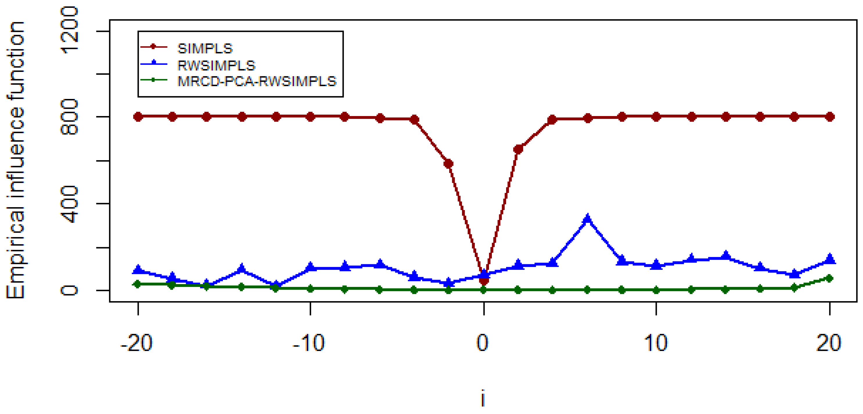
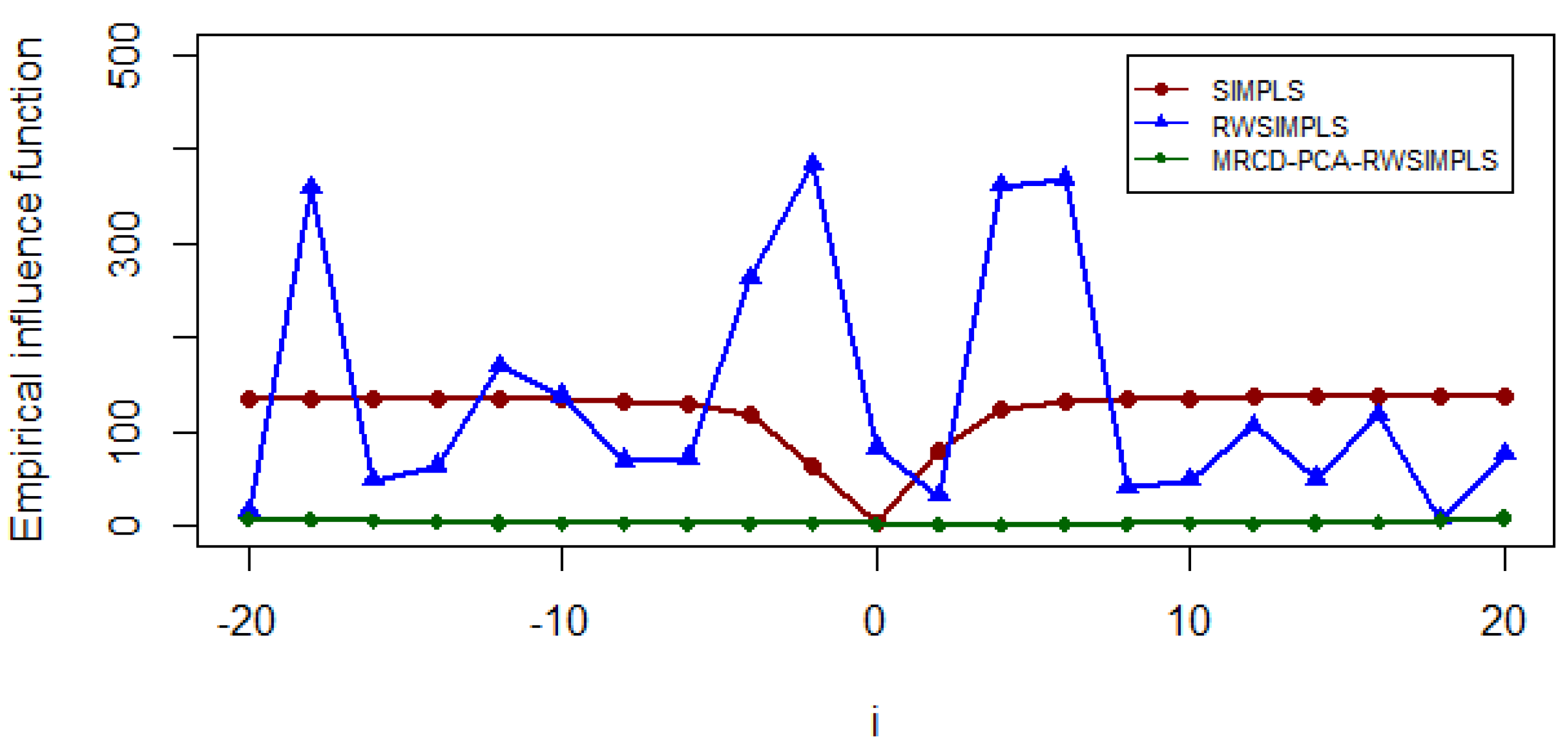
Although RWSIMPLS has been shown to be more efficient than the SIMPLS, it is suspected that it is not efficient enough due to using weighting functions in Equation (15) in the RWSIMPLS procedure. The main aim of using the weighting function in the RWSIMPLS algorithm is to reduce the effect of outliers, especially HLPs. However, no identification of HLPs method is considered when defining the weight function. Instead, [16] employed weight function as in Equation (15), which is based on the residual, model density, and function distribution but is not based on any method of the identification of HLPs. As a result, there is no guarantee that the weight they proposed will lessen the impact of true HLPs on the parameter estimates, and this will produce a misleading conclusion. This limitation prompted us to propose a new version of RWSIMPLS, which is based on the MRCD-PCA method of identification of HLPs for HDD, denoted as MRCD-PCA-RWSIMPLS. We expect that this method will be more efficient than SIMPLS and RWSIMPLS.

3. The Proposed MRCD-PCA-RWSIMPLS Algorithm

In this section, we introduce our new proposed MRCD-PCA-RWSIMPLS procedure. We first describe how the weighting function is formulated. Then, the full algorithm of the proposed method is illustrated.

3.1. Formulating the Weighting Function

The diagnostic robust Mahalanobis distance based on the combination of minimum regularized covariance determinant and principal component analysis (RMD(MRCD-PCA)) method is expected to be very successful in the detection of multiple HLPs in high dimensional data with sparse structures.

The method consists of three steps whereby, in the first step, the dimension of a high dimensional sparse dataset will be reduced by using the PCA method. The idea to exploit PCA is to replace the original $X$ matrix with k largest eigenvalues to the corresponding eigenvectors. In the second step, we generate a fitted $\widehat{X}$ matrix in the original dimension $p$ based on the chosen number of principal components such that its cumulative variance is at least 80%. In the third step, the fitted $\widehat{X}$ matrix will be shrunk, and an invertible covariance matrix for HDD is yielded. The MRCD [18] was then performed on these fitted $\widehat{X}$ to determine the robust mean and robust covariance of HDD. By using these robust estimators, the distance of each observation was computed by employing the Robust Mahalanobis Distance (RMD) based on MRCD-PCA.

The advantage of this method is that data are transformed based on the orthogonal PCA components, and it can reduce noise and solve the multicollinearity issue without losing much information. We have the following estimated:

MRCD-PCA location estimates:

$$M_{mrcd\text{-}pca}=V_{\hat{x}}+D_{\hat{x}}{m}_{\hat{u}}(H_{mrcd\text{-}pca})$$

(27)

MRCD-PCA scatter estimates:

$$K_{mrcd\text{-}pca}=D_{\hat{x}}{Q\mathsf{\Lambda }}^{-\frac{1}{2}}\left[\rho I+(1-\rho )S_{\hat{w}}(H_{mrcd\text{-}pca})\right]{\mathsf{\Lambda }}^{-\frac{1}{2}}{Q^{\prime }D}_{\hat{x}}$$

(28)

where $m_{\widehat{u}}(H_{mrcd\text{-}pca})$ is a location estimate based on subset $H_{mrcd\text{-}pca}$, $D_{\widehat{x}}$ is a diagonal matrix scale for each independent variables, $V_{\widehat{x}}$ is vector mean for each independent variable, $\rho$ is a regularization parameter, $Q$ is an eigenvector of identity matrix, $\mathsf{\Lambda }$ is an eigenvalue of identity matrix, $I$ is an identity matrix, $H_{mrcd\text{-}pca}$ is a subset of data points with smallest determinant, and $S_{\widehat{w}}(H_{mrcd\text{-}pca})$ is a sample covariance of $H_{mrcd\text{-}pca}$.

Following [20], after obtaining robust multivariate location and scale estimates given by MRCD, we compute the Robust Mahalanobis Distance (RMD) as follows:

$${RMD}_i(MRCD\text{-}PCA)=\sqrt{{({\hat{x}}_i-{\hat{\mu }}_{mrcd\text{-}pca})}^T{\mathsf{\Sigma }}_{mrcd\text{-}pca}^{-1}({\hat{x}}_i-{\hat{\mu }}_{mrcd\text{-}pca})}$$

(29)

where ${\widehat{\mu }}_{mrcd\text{-}pca}$ and ${\mathsf{\Sigma }}_{mrcd\text{-}pca}^{-1}$ are the estimates of the robust mean and robust covariance matrix of MRCD-PCA, respectively. Since the distribution of $RM{D}_i(MRCD\text{-}PCA)$ is intractable, as per [20], we use a confidence bound type cut-off point as follows.

$${(cut\text{-}off)}_{mrcd\text{-}pca}=median({RMD}_{mrcd\text{-}pca})+3MAD({RMD}_{mrcd\text{-}pca})$$

(30)

Any observation that corresponds to $RM{D}_i(MRCD\text{-}PCA)$ exceeding this cut-off point is considered as HLPs. Following [21,22], a weight function is formulated based on the diagnostic method of the detection of outliers with the main aim of reducing their effect on the parameter estimates. Thus, we formulate a new weight function based on $RM{D}_i(MRCD\text{-}PCA)$ as follows:

$$w_{mrcd\text{-}{pca}_i}=\left[1,\frac{{(cut\text{-}off)}_{mrcd\text{-}pca}}{{RMD}_{mrcd\text{-}{pca}_i}}\right]$$

(31)

where weight equals to $\frac{{(cut-off)}_{mrcd\text{-}pca}}{RM{D}_{mrcd\text{-}pc{a}_i}}$ is given to leverage points, and a weight equal to 1 is given to regular observations. Subsequently, this weight is integrated in the establishment of the MRCD-PCA-RWSIMPLS algorithm.

In our proposed algorithm, we scaled the dataset, $x_{ij}$, by using robust weighted mean, ${\overline{x}}_j{}^w$, and robust weighted standard deviation, $S_j{}^w$. The empirical covariance in our algorithm is computed based on the robust scaled weighted dataset, $X^w$ and $Y^w$. Then, we extract PLS-components by deflating a robust scaled weighted covariance matrix, $C^w=X^{w^T}{Y}^w$.

3.2. The Proposed Algorithm of MRCD-PCA-RWSIMPLS

Step 1: Calculate the weights as in Equation (31) and store them in a diagonal matrix.

Step 2: Compute the robust weighted mean and robust weighted standard deviation for each column of $X$ and column of $Y$ matrices:

$${\overline{x}}_j^w=\frac{{\displaystyle {\displaystyle \sum }_{i=1}^n}{w}_{mrcd\text{-}{pca}_i}{x}_{ij}}{{\displaystyle {\displaystyle \sum }_{i=1}^n}{w}_{mrcd\text{-}{pca}_i}} for j=1,\dots ,p and i=1,\dots ,n$$

(32)

$$s_j^w=\frac{{\displaystyle {\displaystyle \sum }_{i=1}^n}{w}_{mrcd\text{-}{pca}_i}(x_{ij}-{\overline{x}}_j^w)}{{\displaystyle {\displaystyle \sum }_{i=1}^n}{w}_{mrcd\text{-}{pca}_i}-1} for j=1,\dots ,p and i=1,\dots ,n$$

(33)

$${\overline{y}}^w=\frac{{\displaystyle {\displaystyle \sum }_{i=1}^n}{w}_{mrcd\text{-}{pca}_i}{y}_i}{{\displaystyle {\displaystyle \sum }_{i=1}^n}{w}_{mrcd\text{-}{pca}_i}} for i=1,\dots ,n$$

(34)

$$s_y^w=\frac{{\displaystyle {\displaystyle \sum }_{i=1}^n}{w}_{mrcd\text{-}{pca}_i}(y_i-{\overline{y}}^w)}{{\displaystyle {\displaystyle \sum }_{i=1}^n}{w}_{mrcd\text{-}{pca}_i}-1} for i=1,\dots ,n$$

(35)

where ${\overline{x}}_j^w$ is a robust weighted mean of column $X$, $s_j^w$ is a robust weighted standard deviation of column $X$, ${\overline{y}}^w$ is a robust weighted mean of column $Y$, and $s_y^w$ is a robust weighted standard deviation of column $Y$.

Step 3: Center and scale each of the data, $x_{ij}$ and $y_i$, by using robust weighted mean and robust weighted standard deviation in Step 2.

$$x_{ij}^w=\frac{x_{ij}-{\overline{x}}_j^w}{s_j^w}$$

(36)

$$y_i^w=\frac{y_i-{\overline{y}}^w}{s_y^w}$$

(37)

Step 4: Determine the robust weighted covariance based on the weighted scaled observations in step 3.

$$C^w=X^{w^T}{Y}^w$$

(38)

Step 5: Perform ordinary SIMPLS as in Section 2.1 on robust scaled weighted dataset, $X^w$ and $Y^w$, by using the robust weighted scaled covariance, $C^w$, in Step 4 to determine the estimated coefficients.

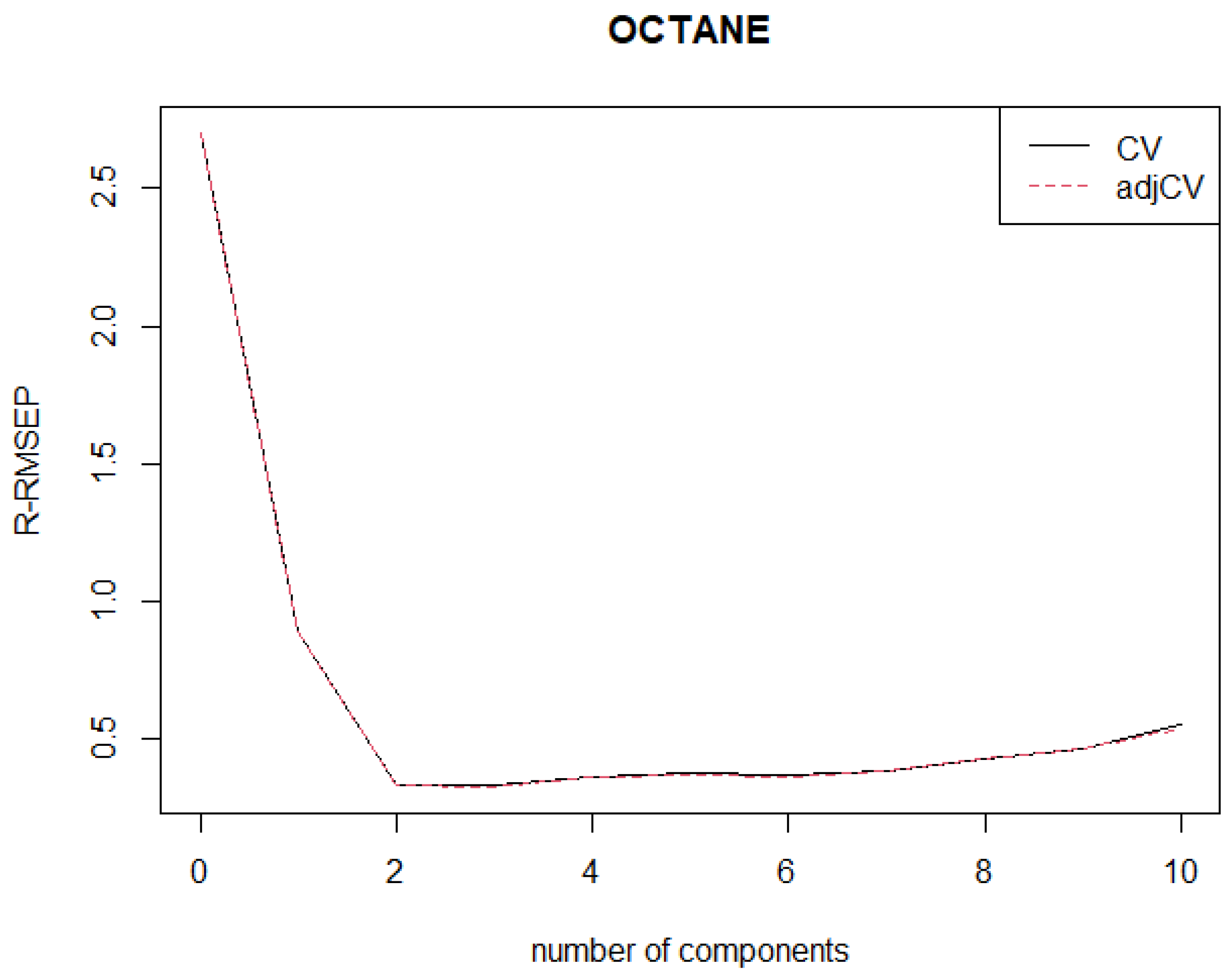
Step 6: Note that Steps 4 to 5 are repeated for all $k$, i.e., the optimal number of components selected based on robust root mean squared error prediction $R-RMSE{P}_k$. We call this algorithm a robust weighted SIMPLS based on MRCD-PCA (MRCD-PCA-RWSIMPLS).

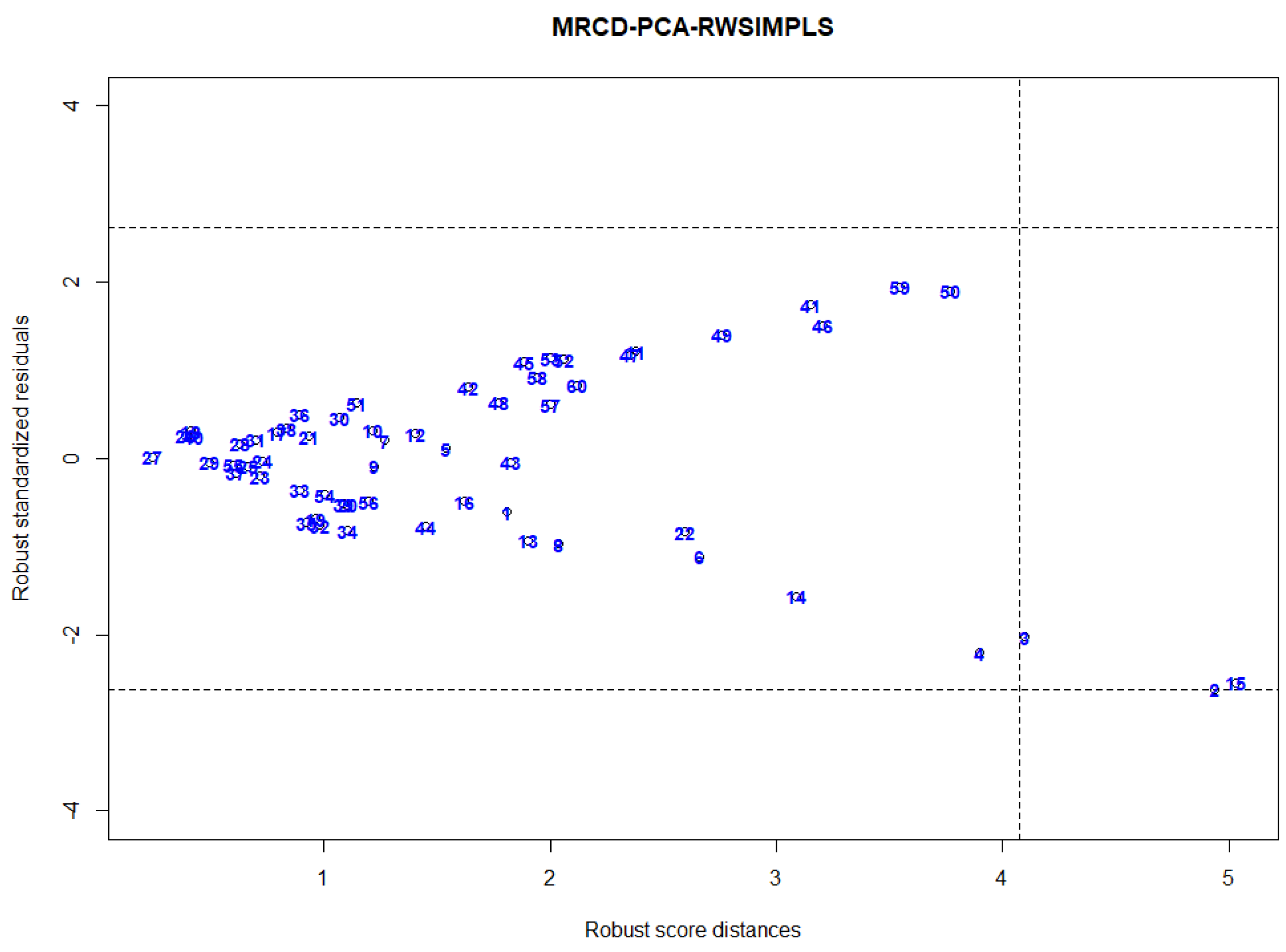
3.3. The Proposed Diagnostic Plots Based on MRCD-PCA-RWSIMPLS

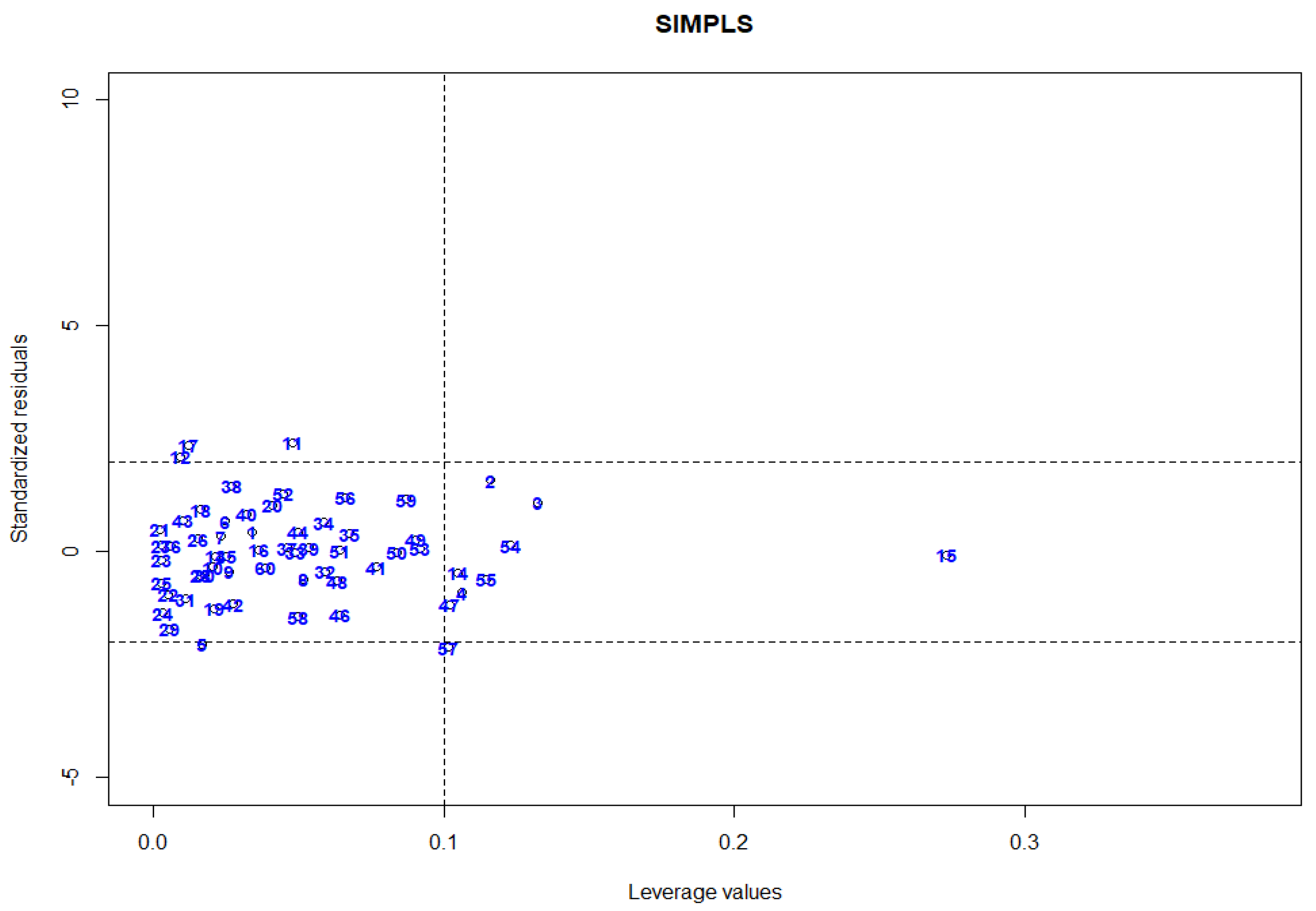
A diagnostic plot is very useful for practitioners to quickly capture abnormalities in data. Rousseeuw and Zomeren [23] established a diagnostic plot to classify observations into four types of data points, namely regular observations, good leverage points, vertical outliers, and bad leverage points. The proposed plot plots the standardized residual versus squared robust Mahalanobis distance based on minimum volume ellipsoid (MVE) or minimum covariance determinant (MCD). In PLS regression analysis, orthogonal, score, and residual distance can be used to measure the degree of outlyingness of an observation [14]. 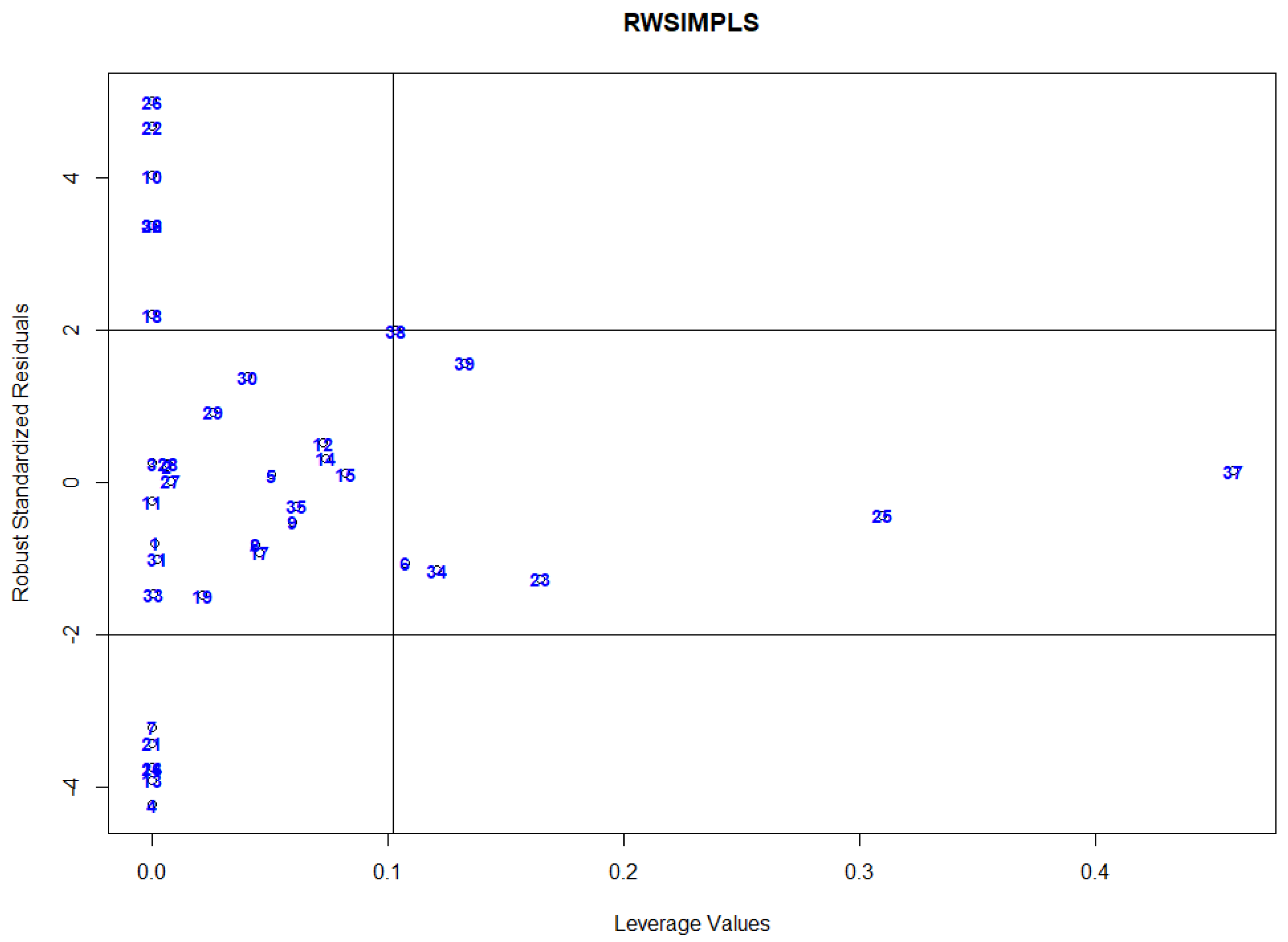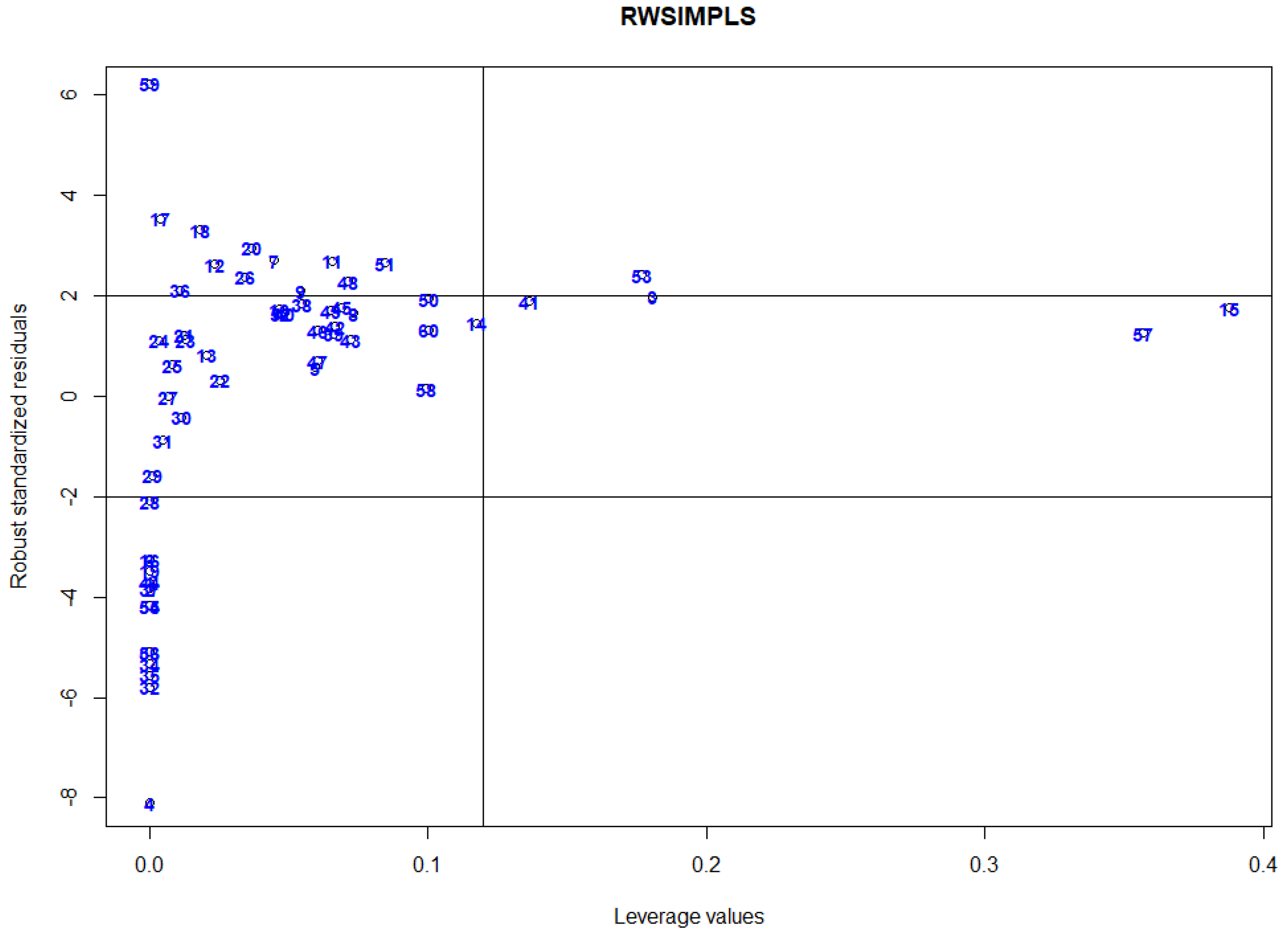Aylin and Agostinelli [16] proposed a diagnostic plot to classify observations into four types of data points by plotting RWSIMPLS standardized residuals versus leverage values, i.e., the diagonal elements of the hat matrix that is used to identify HLPs. Any observation that corresponds to a leverage value larger than the cut-off points, 2p/n, is considered as HLPs. 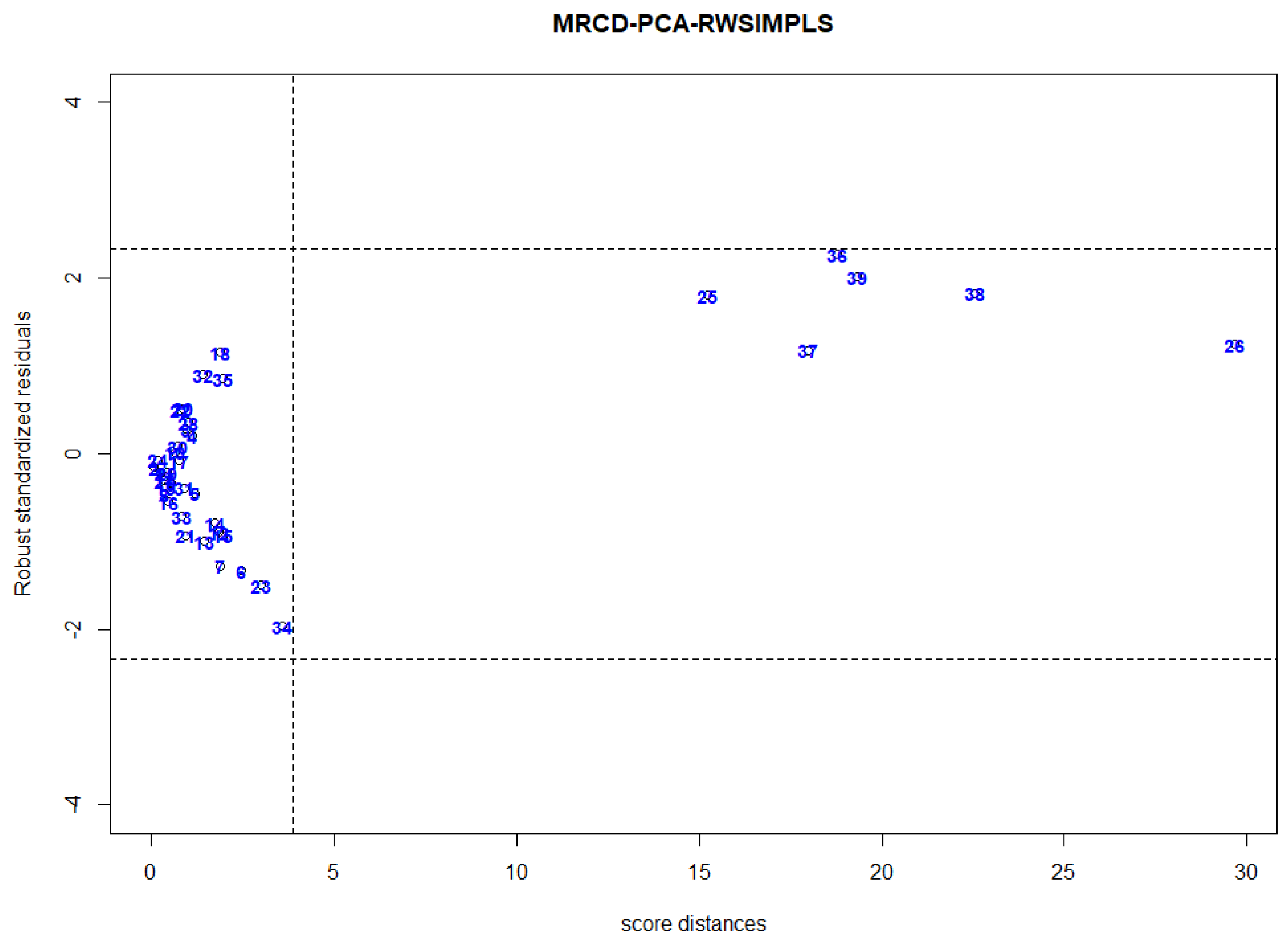The disadvantage of this plot is that it employs leverage values that are proven to not be very successful in detecting multiple HLPs due to the masking effect [24]. Hence, using leverage values as diagnostic measure for identifying HLPs will produce unsatisfactory results. Thus, we propose a new diagnostic plot by plotting the MRCD-PCA-RWSIMPLS standardized residual against the robust Mahalanobis distance as in Equation (29) and cut-off point as in Equation (30).

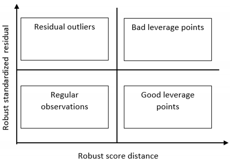
The robust standardized residual-score distance plot is a scatter plot of the robust standardized residual versus the robust diagnostic measure for identifying HLPs. The vertical axis of the graph is the robust standardized residual, and the horizontal axis is the robust score distance, as described Equation (29). The standardized robust residual and robust score distance threshold lines are also shown on the plot to indicate the existence and the types of outliers. Based on the robust standardized residual-score distance plot, we can categorize observations into four categories:

• Observations in the lower-left corner are “regular observations”
• In the upper left corner are the observations that are far away from the $y$ space and the observations that have large robust standardized residuals. These points are known as “vertical outliers”
• Observations in the lower right corner are “good leverage points” The points are far from the PLS space but proceed in the direction of the fitted line. These observations have a large robust score distance with a small robust standardized residual.
• Observations in the upper right corner are “bad leverage points” that have large robust standardized residual and large robust score distances.

It is important to highlight the difference between Rousseeuw and Zomeren [23] and our proposed diagnostic plots. The diagnostic plot proposed by Rousseeuw and Zomeren [23] plots standardized least trimmed squares residuals on the Y-axis while the robust Mahalanobis distance based on minimum volume ellipsoid (MVE) or minimum covariance determinant (MCD) is plotted on the X-axis. This plot can only be used for low dimensional data. Our proposed MRCD-PCA-RWSIMPLS diagnostic plot plots the MRCD-PCA-RWSIMPLS standardized residuals against the robust score distance based on the MRCD-PCA diagnostic measure for identifying HLPs for HDD. Our proposed plot can be applied to both low and high dimensional data.

4. Results and Discussion

This section reports an extensive Monte Carlo simulation study and the analysis of two real datasets in order to assess the performance of our proposed MRCD-PCA-RWSIMPLS compared to SIMPLS and RWSIMPLS methods. All computations were performed using R software.

4.1. Simulation Study

The simulation study was conducted similarly to [16]’s simulation design. The $i^{th}$ observation for the response variable is obtained by $y_i=x_i\beta +e_i$ where $x_i=(x_{i1},x_{i2},\dots x_{ik})$, $i=1,2,..,n$. A true parameter $\beta$ is drawn from a normal distribution with a mean of 0 and a standard deviation of 0.001. The explanatory variable matrix $X$ is calculated by $X=T{P}^T$ so that the rank of $X$ equals the number of components $K$, which is the number of columns T; T is matrix of $n\times k$, and P is a matrix of $p\times k$. The columns of $P$ and $T$ are generated from the standardized normal distribution, $p_k~N(0,1)$ and $t_k~N(0,1)$, where $k$ is the number of components, $k=1,2,3,\dots ,K$, and $e_i$ is drawn from N(0, 1).

In this study, we consider an asymmetric contamination scenario for two cases under a Student’s t-distribution with 2 degrees of freedom $(t_2)$ and Student’s t-distribution with 5 degrees of freedom $(t_5)$. In the first case, we contaminate the data in the X direction by generating three different proportions of outliers, $\epsilon$, such as 10%, 20%, and 30%, given the contamination models for Student’s t-distribution with 2 and 5 degrees of freedom, i.e., $X~(1-\epsilon )N(0,1)+\epsilon (t_2)$ and $X~(1-\epsilon )N(0,1)+\epsilon (t_5)$, respectively. In the second case, we contaminate the data in both the $X$ and $Y$ directions by generating the same percentage of outliers as in the first case. The contamination model can be written as $X~(1-\epsilon )N(0,1)+\epsilon (t_2)$ and $Y~(1-\epsilon )N(0,1)+\epsilon (t_2)$ for Student’s t-distribution with 2 degrees of freedom and $X~(1-\epsilon )N(0,1)+\epsilon (t_5)$ and $Y~(1-\epsilon )N(0,1)+\epsilon (t_5)$ for Student’s t-distribution with 5 degrees of freedom. In order to investigate the effect of different sizes and different number of predictors on the MRCD-PCA-RWSIMPLS estimates, four samples of different sizes (30, 60, 100, and 200) and different number of predictors (100, 400, 800, and 1000) were considered, and under each setting, we repeat the simulation 1000 times, i.e., S = 1000. Following [16] the optimal number of components, A is fixed as two for each setting. As per Aylin and Agostinelli [16], the Mean squared error (MSE) for $\widehat{\beta }$, i.e., $MSE=\frac{1}{S}{\displaystyle \sum }\Vert {\widehat{\beta }}^s-{\beta }_0{\Vert }^2$, is used as a criterion to evaluate the performance of our proposed MRCD-PCA-RWSIMPLS compared to the existing SIMPLS and RWSIMPLS estimators. MSE can easily be shown to have two components: one measures variability (precision), and the other measures its bias (accuracy). A good estimator is one that has the least MSE. The results are presented in Table 1 and Table 2.

Table 1. Mean square errors for regression parameter estimates. Contamination in $X$ direction.

Percentage	Dataset	Contamination	MRCD-PCA-RWSIMPLS	SIMPLS	RWSIMPLS
$10\%$	$30\times 100$	$t_2$	0.00474	0.16121	0.06745
		$t_5$	0.00195	0.28263	0.07529
	$60\times 400$	$t_2$	0.00168	0.06214	0.01430
		$t_5$	0.00220	0.14570	0.03876
	$100\times 800$	$t_2$	0.00252	0.03934	0.01751
		$t_5$	0.00213	0.12251	0.04608
	$200\times 1000$	$t_2$	0.00324	0.03479	0.01314
		$t_5$	0.00277	0.19720	0.08660
$20\%$	$30\times 100$	$t_2$	0.00329	0.09638	0.01958
		$t_5$	0.00323	0.26193	0.05962
	$60\times 400$	$t_2$	0.00194	0.02915	0.00641
		$t_5$	0.00164	0.13919	0.04685
	$100\times 800$	$t_2$	0.00198	0.01706	0.00821
		$t_5$	0.00257	0.11812	0.04264
	$200\times 1000$	$t_2$	0.00198	0.01461	0.00421
		$t_5$	0.00321	0.18562	0.08467
$30\%$	$30\times 100$	$t_2$	0.00476	0.06181	0.012623
		$t_5$	0.00375	0.25024	0.06458
	$60\times 400$	$t_2$	0.00196	0.01830	0.00553
		$t_5$	0.00229	0.13011	0.05796
	$100\times 800$	$t_2$	0.00191	0.01060	0.00343
		$t_5$	0.00187	0.11145	0.04180
	$200\times 1000$	$t_2$	0.00324	0.01077	0.00425
		$t_5$	0.00332	0.17711	0.06910

Table 2. Mean square errors for regression parameter estimates. Contamination in $X$ and $Y$ directions.

Percentage	Dataset	Contamination	MRCD-PCA-RWSIMPLS	SIMPLS	RWSIMPLS
$10\%$	$30\times 100$	$t_2$	0.00231	0.20613	0.04595
		$t_5$	0.00233	0.20613	0.08047
	$60\times 400$	$t_2$	0.00149	0.06427	0.02540
		$t_5$	0.00212	0.06427	0.04102
	$100\times 800$	$t_2$	0.00175	0.03903	0.01619
		$t_5$	0.00187	0.12910	0.04354
	$200\times 1000$	$t_2$	0.00166	0.05550	0.01911
		$t_5$	0.00282	0.32877	0.01911
$20\%$	$30\times 100$	$t_2$	0.00122	0.40328	0.01671
		$t_5$	0.00254	0.28565	0.01671
	$60\times 400$	$t_2$	0.00193	0.05798	0.01316
		$t_5$	0.00208	0.15039	0.01316
	$100\times 800$	$t_2$	0.00095	0.09147	0.00716
		$t_5$	0.00195	0.12677	0.04033
	$200\times 1000$	$t_2$	0.00162	0.04694	0.01093
		$t_5$	0.00165	0.14273	0.02664
$30\%$	$30\times 100$	$t_2$	0.00237	0.39527	0.00662
		$t_5$	0.00392	0.27682	0.06037
	$60\times 400$	$t_2$	0.00130	0.09185	0.00450
		$t_5$	0.00149	0.14653	0.03940
	$100\times 800$	$t_2$	0.00144	0.11145	0.0043
		$t_5$	0.00155	0.12823	0.03783
	$200\times 1000$	$t_2$	0.00213	0.07274	0.00576
		$t_5$	0.00233	0.14222	0.02767

It can be observed from Table 1 and Table 2 that MRCD-PCA-RWSIMPLS is the most efficient method evidenced by having the least MSE values followed by RWSIMPLS and SIMPLS irrespective of error distributions, sample size, outlier direction, and percentage of contamination. We observe that the classical SIMPLS performs poorly.

In the following section, the performance of our proposed MRCD-PCA-RWSIMPLS was further evaluated with regards to its classification of observations into four categories and empirical influence functions using two real datasets.

4.2. Gasoline Dataset

The Gasoline dataset contains 401 near-infrared (NIR) spectroscopy measurements ($x$-variables) from 900 nm to 1700 nm with 60 gasoline samples. The response element is the Octane number of 83.4 to 89.6. Mevik and Wehren [25] noted that this dataset contains no outliers. Branden and Hubert [26] used the same dataset to compare the performance of SIMPLS and the RSIMPLS methods for the empirical influence function. Aylin and Agostinelli [16] also employed this dataset in their study in order to compare the performance of their proposed RWSIMPLS compared to SIMPLS and PRM methods.

In building the PLS regression model, it is very crucial to select the optimal number of components, $k$ [27]. The most popular method used is the leave one out cross-validation (LOOCV) for choosing the appropriate number of PLS components [28]. Data are divided into a test and a training set. The test set is used to estimate the regression parameters and should be independent of the training set. The root mean squared error prediction $RMSE{P}_k$ is computed for each number of PLS components, and $k$ in the test set. $RMSEP$ is used to choose the appropriate number of PLS components. It is defined as $RMSE{P}_k=\sqrt{\frac{1}{n_t}{\displaystyle {\displaystyle \sum }_{i=1}^{n_t}}{(y_i-{\widehat{y}}_{i(k)})}^2}$ where $y_i$ is the respondent observation in the dataset, and ${\widehat{y}}_{i(k)}$ is the estimated values of respondent observation in the test set with $k$ PLS components.

In order to determine the optimal number of components, SIMPLS based on leave one out cross-validation (LOOCV) root mean square error is calculated for k = 1, 2, 3, …, and 10 components and the scree plot is obtained. We divide the dataset into train and test datasets. For gasoline data, we take $n_{train}=50$ and $n_{test}=10$ with 10 components. In this paper, we also propose a robust root means square error prediction $R\text{-}RMSE{P}_k=\sqrt{\frac{1}{n_{test}}{\displaystyle {\displaystyle \sum }_{i=1}^{n_t}}{(y_i-{\widehat{y}}_{MRCD\text{-}PCA\text{-}WSIMPL{S}_{i(k)}})}^2}$ where $y_i$ is the respondent observation in the dataset, and ${\widehat{y}}_{MRCD\text{-}PCA\text{-}WSIMPL{S}_{I(K)}}$ is the predicted values based on MRCD-PCA robust weighted SIMPLS observations in the test set. R-RMSEP is compared to the classical RMSEP, and the results are shown in Table 3 and Table 4. Based on Table 4, the optimal number of components chosen is k = 3, which explains 95.78 percent of the variation in Gasoline data, and this total variance is yielded by R-RMSEP. Likewise, in Table 3, R-RMSEP provides a low error value of 0.264. The scree plot of R-RMSEP in Figure 1 indicates that there is a significant drop from PLS component one to PLS component three, and after PLS component three, the graph line shows no changes and is almost flat. On the other hand, the scree plot of classical RMSEP in Figure 2 shows that there is a sharp elbow occurring at component two. However, as observed in Table 4, the classical RMSEP only indicates 85.58 percent of total variance explained for component two, which is less than the total variance computed by R-RMSEP with three components. Hence, $k=3$ is chosen as the number of components after which the cross-validation error does not show a significant decrease [25], and the total variance explained is more than 90 percent as suggested by [29]. We use the number of components equals to three to perform our proposed diagnostic plot on this dataset in order to classify the outlying observations into three types of outliers.

Table 3. Leave one out cross validation of R-RMSEP and classical RMSEP for Gasoline data.

Cross-Validated Using 50 Leave One Out Segments
	Intercept	1 Comp	2 Comps	3 Comps	4 Comps	5 Comps	6 Comps	7 Comps	8 Comps	9 Comps	10 Comps
R-RMSEP	1.344	1.140	0.658	0.264	0.207	0.226	0.214	0.227	0.259	0.269	0.267
RMSEP	1.545	1.357	0.297	0.252	0.248	0.240	0.232	0.239	0.232	0.245	0.267

Table 4. Percentage of variance explained of independent variables $(X)$ and response variable $(Y)$ for Gasoline data.

TRAINING: % Variance Explained
		1 Comp	2 Comps	3 Comps	4 Comps	5 Comps	6 Comps	7 Comps	8 Comps	9 Comps	10 Comps
X	R-RMSEP	62.14	83.06	95.78	97.21	97.59	98.27	98.72	98.83	99.16	99.26
	RMSEP	78.17	85.58	93.41	96.06	96.94	97.89	98.38	98.85	99.02	99.19
Y	R-RMSEP	33.19	81.43	97.07	98.37	98.82	98.92	99.02	99.32	99.41	99.55
	RMSEP	29.39	96.85	97.89	98.26	98.96	98.96	99.09	99.16	99.28	99.39

Figure 1. Scree plot for R-RMSEP for Gasoline data.

Figure 2. Scree plot for RMSEP for Gasoline data.

The diagnostic plots for SIMPLS, RWSIMPLS, and MRCD-PCA-RWSIMPLS are presented in Figure 3, Figure 4 and Figure 5. It can be observed from Figure 4 that the plot based on RWSIMPLS produces erroneous results because many good observations are declared as outliers. This phenomenon is referred to a swamping effect. The RWSIMPLS plot declared observations 3, 15, 41, and 57 as good leverage points, observation 53 as a bad leverage point, and observations 1, 2, 4, 6, 7, 9, 11, 12, 16, 17, 18, 19, 20, 26, 28, 32, 33, 34, 35, 36, 37, 44, 48, 51, 54, 55, 56, and 59 as vertical outliers. The plot in Figure 5 based on SIMPLS also shows the swamping effect whereby it declared eight good HLPs, i.e., cases 2, 3, 4, 14, 15, 47, 54, and 55. There is one bad HLPs for observation 57 and four vertical outliers for observations 5, 11, 12, and 17. However, it is interesting to observe the plot in Figure 3, which is based on our proposed MRCD-PCA-RWSIMPLS. It shows less swamping effects where it only declared three good leverage points on observations 2, 3, and 15. Thus, our proposed MRCD-PCA-RWSIMPLS plot is more reliable than the other two plots.

Figure 3. Diagnostic plot of MRCD-PCA-RWSIMPLS for Gasoline data.

Figure 4. Diagnostic plot of RWSIMPLS for Gasoline data.

Figure 5. Diagnostic plot of SIMPLS for Gasoline data.

The performance of MRCD-PCA-RWSIMPLS method is further evaluated with regard to its empirical influence function.

Influence Function

Following [16], the empirical influence function was constructed by first scaling the dependent variable ($Y$) to have a similar range with predictor variables. Next, in order to contaminate the dataset, we substitute the first explanatory variable $x_{11}$ and the first dependent variable $y_1$ with the value from −20 to 20 simultaneously. Then, the empirical influence function is calculated by Equation (39):

$$\Vert \frac{{\hat{\beta }}_c-\hat{\beta }}{\raisebox{1ex}{$1$}\!\left/ \!\raisebox{-1ex}{$n$}\right.}\Vert$$

(39)

where ${\widehat{\beta }}_c$ is the estimated coefficient parameter obtained from the contaminated dataset, $\widehat{\beta }$ is the estimated coefficient parameter of clean dataset, and $n$ is equals to 60.

Figure 6 demonstrates the results of empirical influence functions for SIMPLS, RWSIMPLS, and our proposed MRCD-PCA-RWSIMPLS method. We observe that the empirical influence function for SIMPLS is much affected when we replaced the first value of the response and explanatory variables with 0. It can be observed that SIMPLS has the largest empirical influence values, and its plot plunges at $x_{11}$ = 0 and $y_1$ = 0 and produces a small value of influence function at that point, similar to those of RWSIMPLS and MRCD-PCA-RWSIMPLS. It is interesting to observe that the MRCD-PCA-RWSIMPLS has the lowest empirical influence values and shows no fluctuation in its estimates. On the contrary, the empirical influence values for RWSIMPLS are higher than MRCD-PCA-RWSIMPLS, with moderate fluctuations.

Figure 6. Empirical influence functions of SIMPLS (red line), RWSIMPLS (blue line), and MRCD-PCARWSIMPLS (green line) for Gasoline data.

4.3. Octane Dataset

The second real example in this paper is the octane dataset where it contains near-infrared (NIR) and absorbance spectra over p = 226 wavelengths with n = 39 gasoline samples. Leave one out cross validation (LOOCV) is performed to determine the optimal number of components, SIMPLS for k = 1, 2, 3, …, 10 components, and the scree plot is obtained. The robust root mean squares error predicted (R-RMSEP) is computed. We first divide the dataset into train and test datasets. For octane data, we take $n_{train}=30$ and $n_{test}=9$ with 10 components. From the scree plot in Figure 7, it can be observed in the R-RMSEP plot that there is a substantial drop from component one to component two, and after component two, the graph line shows no major changes. Moreover, in Table 5, the R-RMSEP produces a smaller root mean square error of 0.576 compared to classical RMSEP. In Table 6, the two components of R-RMSEP explained almost 80 percent of the total variance in Octane data. Therefore, it is adequate to choose the number of components as equals to two for the Octane dataset. On the contrary, the classical RMSEP in Figure 8 shows the lowest point in the graph is on the third component, and there is a fluctuation in the line. It indicates that the classical RMSEP is intruded by the outliers in the Octane dataset. Based on Table 4, the third component of classical RMSEP produces very high variance explained at 99.06 percent, which is almost 100 percent of data explained, and this can cause overfitting as the classical RMSEP is influenced by outliers [30].

Figure 7. Scree plot of R-RMSEP for Octane data.

Table 5. Leave one out cross validation for R-RMSEP and classical RMSEP for Octane data.

Cross-Validated Using 30 Leave One Out Segments
	Intercept	1 Comp	2 Comps	3 Comps	4 Comps	5 Comps	6 Comps	7 Comps	8 Comps	9 Comps	10 Comps
R-RMSEP	1.643	0.943	0.576	0.573	0.601	0.612	0.603	0.621	0.655	0.683	0.740
RMSEP	2.105	2.116	0.738	0.282	0.390	0.535	1.297	1.310	0.752	0.492	0.356

Table 6. Percentage of variance explained of independent variables $(X)$ and response variable $(Y)$ for Octane data.

TRAINING: % Variance Explained
		1 Comp	2 Comps	3 Comps	4 Comps	5 Comps	6 Comps	7 Comps	8 Comps	9 Comps	10 Comps
X	R-RMSEP	63.96	79.60	90.23	95.32	96.67	97.96	98.51	99.32	99.71	99.84
	RMSEP	53.65	97.55	99.06	99.15	99.80	99.90	99.92	99.97	99.99	99.99
Y	R-RMSEP	69.99	90.51	92.32	93.01	93.97	94.43	94.99	95.25	95.69	96.53
	RMSEP	50.51	89.27	98.5	99.16	99.21	99.30	99.51	99.58	99.64	99.74

Figure 8. Scree plot of RMSEP for Octane data.

We also illustrate our proposed diagnostic plot on this dataset to classify outlying observations and to compare the robustness of our proposed algorithm, MRCD-PCA-RSIMPLS, and the other two methods, RWSIMPLS and classical SIMPLS. The authors of [18,31] used this dataset to identify outliers, and they diagnosed six outliers in X-space. The outliers are the observations that contain added ethanol. From Figure 9, it is clearly shown that MRCD-PCA-RSIMPLS successfully detects the true six high leverage points (Cases 25, 26, 36, 37, 38, and 39). On the other hand, in Figure 10, the RWSIMPLS method suffers from swamping and masking problems as it detects good observations as outliers, and it fails to detect real outliers. RWSIMPLS declares observations 6, 23, 25, 34, 37, 38 and 39 as good HLPs, vertical outliers for observations 4, 7, 10, 13, 16, 18, 20, 21, 22, 24, 26, 32, and 36. The classical SIMPLS also suffers from masking and swamping effects. As observed, the SIMPLS in Figure 11 identifies observations 23, 26, 36, 37, 38, and 39 as good HLPs and observation 7, 13, and 32 as vertical outliers. SIMPLS suffers from a masking problem as it fails to detect the outlier point on observation 25. MRCD-PCA-RWSIMPLS diagnostic plots are very efficient in detecting and classifying outliers without the masking and swamping problem. However, RWSIMPLS could detect the outlying observation correctly with additional false outliers, whereas the performance of the SIMPLS is even worse. The method fails to detect the true HLPs.

Figure 9. Diagnostic plot of MRCD-PCA-RWSIMPLS for Octane data.

Figure 10. Diagnostic plot of RWSIMPLS for Octane data.

Figure 11. Diagnostic plot of SIMPLS for Octane data.

Influence Function

In order to compute the empirical influence function for Octane data, we first removed the six outliers for observations 25, 26, 36, 37, 38, and 39 from the dataset in order to avoid distracting errors in the influence function computation. Data are then contaminated in the same manner as that of [16] by simultaneously replacing the first explanatory variable and the first dependent variable with values ranging from −20 to 20. The empirical influence function is calculated as in Equation (39). Figure 12 displays the graphical result of empirical influence functions for SIMPLS, RWSIMPLS, and our proposed MRCD-PCA-RWSIMPLS method. We observe that the empirical influence function for the SIMPLS is affected when we replaced the first value of the response and the explanatory variables with 0. It can be observed that SIMPLS has the large empirical influence values and its plot plunges at $x_{11}$ = 0 and $y_1$ = 0 and provides a small value of influence function at that point. The performance of RWSIMPLS is terrible as it fluctuates tremendously when the data are corrupted. It shows that RWSIMPLS is extremely vulnerable to even a single outlier in the data. It is interesting to observe that MRCD-PCA-RWSIMPLS has the lowest empirical influence values and shows no fluctuation in its estimates.

Figure 12. Empirical influence functions of SIMPLS (red line), RWSIMPLS (blue line), and MRCD-PCARWSIMPLS (green line) for Octane data.

5. Conclusions

In this paper, a robust weighted of SIMPLS, which is based on weight obtained from MRCD-PCA was developed. We call this method MRCD-PCA-RWSIMPLS. A new diagnostic plot for classifying observations into four types of data points, namely regular observations, good leverage points, vertical outliers, and bad leverage points, is also established. The robust weighting function introduced in the algorithm of MRCD-PCA-RWSIMPLS has tremendously improved the efficiency of its estimates. The MRCD-PCA-RWSIMPLS outperformed the SIMPLS and RWSIMPLS methods as it has the least MSE and the least empirical influence value. SIMPLS produced the worst performance. The proposed MRCD-PCA-RWSIMPLS diagnostic plot was able to classify observations into correct groups. SIMPLS and RWSIMPLS diagnostic plots failed to correctly identify the actual type of data points and suffered from masking and swamping effects. Hence, the merits of our proposed MRCD-PCA-RWSIMPLS method and its diagnostic plot are confirmed, as reflected in their application to real datasets and in the Monte Carlo simulation study. Nonetheless, our proposed MRCD-PCA-RWSIMPLS method has its own limitation as its computation running time is slightly longer than that of SIMPLS and RWSIMPLS methods. A slightly increased running time for obtaining MRCD-PCA-RWSIMPLS estimates compared to the other two methods is a trade-off one has to consider when using our proposed method as it is the most efficient method for confronting outliers for HDD.