Modeling RL Electrical Circuit by Multifactor Uncertain Differential Equation

Abstract

The symmetry principle of circuit system shows that we can equate a complex structure in the circuit network to a simple circuit. Hence, this paper only considers a simple series RL circuit and first presents an uncertain RL circuit model based on multifactor uncertain differential equation by considering the external noise and internal noise in an actual electrical circuit system. Then, the solution of uncertain RL circuit equation and the inverse uncertainty distribution of solution are derived. Some applications of solution for uncertain RL circuit equation are also investigated. Finally, the method of moments is used to estimate the unknown parameters in uncertain RL circuit equation.

1. Introduction

For the sake of rationally handling the likelihood that something will happen, uncertainty theory was established by Liu [1] and then perfected by Liu [2]. To this day, uncertainty theory has been extensively studied and has spawned numerous theoretical branches.

Among the theoretical branches of uncertainty theory, an uncertain differential equation is a type of differential equation driven by Liu process. It was first presented by Liu [3] to model the dynamic systems with continuous-time noises. For the purpose of investigating the solution of uncertain differential equation, Chen and Liu [4] first verified the existence and uniqueness theorem of solution of uncertain differential equation under linear growth condition and Lipschitz condition. Later, the theorem was extended to local linear growth condition and local Lipschitz condition by Gao [5]. After that, the first concept of stability of uncertain differential equation was proposed by Liu [2]. Afterwards, Yao and Gao [6] proved some theorems to develop the stability analysis of uncertain differential equation, and then other types of stability were presented by Sheng and Wang [7], Yao et al. [8], Yang et al. [9], etc. As the most significant contribution, the Yao–Chen formula was shown by Yao and Chen [10] to associate uncertain differential equation with ordinary differential equations, which greatly promoted the development of uncertain differential equation. Based on the Yao–Chen formula, the numerical method of solving uncertain differential equation was first presented by Yao and Chen [10], which was then developed by Yang and Shen [11], Yang and Ralescu [12], Gao [13], etc. As a topic that has attracted much attention in recent years, how to estimate the unknown parameters in an uncertain differential equation that fits the observed data as much as possible is a core problem. In order to deal with this problem, Yao and Liu [14] first presented the method of moments to estimate the unknown parameters. After that, several methods were proposed such as generalized moment estimation (Liu [15]), minimum cover estimation (Yang et al. [16]), least squares estimation (Sheng et al. [17]) and maximum likelihood estimation (Liu and Liu [18]). Based on that, uncertain differential equation was used to model the cumulative number of COVID-19 infections in China by scholars such as Lio and Liu [19], Chen et al. [20] and Jia and Chen [21].

As an important research field of physics systems, electrical circuit is nearly everywhere in our lives. To name only a few, electrical circuit is an essential component of power supply network, car, television, and mobile phone. In the actual electrical circuit system, due to the electromagnetic interference of external environment and the dimension error of potential source device, there is always noise in the circuit system (Bennett [22]). In order to study the effect of noise on circuit system, white noise was first used to describe the classification and numerical simulation of electrical circuit by Kampowsky et al. [23]. Later, the noise was modeled as Wiener process and stochastic differential equation was applied in the modeling of electrical circuit by Penski [24], Kolarova [25], Kolarova [26], etc. However, Liu [27] proved that stochastic circuit differential equation would lead to a paradox and suggested that the noise should be modeled by uncertain differential equation.

In order to model the series RL circuit system more reasonably, this paper first proposes the uncertain RL circuit equation based on multifactor uncertain differential equation by considering the external noise and internal noise. The main contributions of this paper are to derive the solution of uncertain RL circuit equation and the inverse uncertainty distributions of solution, supremum of solution and time integral of solution. The overall structure of this paper takes the form of five sections, including this introductory section. Section 2 begins by deriving the uncertain RL circuit equation, and then gives the solution of uncertain RL circuit equation and the inverse uncertainty distribution of solution. Section 3 investigates two applications of solution of uncertain RL circuit equation. In Section 4, parameter estimation for uncertain RL circuit equation is considered and a numerical experiment is provided. Finally, a concise conclusion is given in Section 5, and the future scope of the study is provided in Section 6.

2. Uncertain RL Circuit Equation

Based on the symmetry principle of circuit system, we only consider a simple series RL circuit, which is an electrical circuit composed of a resistor and inductor and is driven by a potential source. The resistance of the resistor R is denoted by r and measured in ohms ($\Omega$), and the inductance of the inductor L is denoted by l and measured in henrys (H). The current through the resistor and inductor at time t is denoted by $I_t$ and measured in amperes (A), the potential source provided to the circuit system is denoted by $F\left(t\right)$ and measured in volts (V).

2.1. Uncertain RL Circuit Model

Next, we will derive the uncertain RL circuit model based on multifactor uncertain differential equation. Let the time interval $[0,t]$ be divided into n subintervals such that

$$0=t_0<t_1<\cdots <t_{n-1}<t_n=t.$$

Then, we write

$${\displaystyle \Delta =\underset{1\le j\le n}{max}(t_j-t_{j-1}).}$$

For each index j with $1\le j\le n$, we consider the behavior of the circuit system in time interval $(t_{j-1},t_j]$. Due to the electromagnetic interference of external environment to the potential source and the dimension error of potential source device, the potential source provided to the circuit system is often affected by some noise, which is modeled by

$${\sigma }_1\frac{C_{1t_j}-C_{1t_{j-1}}}{t_j-t_{j-1}}.$$

Here,

$$\frac{C_{1t_j}-C_{1t_{j-1}}}{t_j-t_{j-1}}$$

is a normal uncertain variable of mean zero and variance one, and ${\sigma }_1>0$ is known as the intensity of noise. Thus, the actual potential source provided to the circuit system is

$$F\left(t_{j-1}\right)+{\sigma }_1\frac{C_{1t_j}-C_{1t_{j-1}}}{t_j-t_{j-1}}$$

when $\Delta$ is sufficiently small. When the current through the resistor, the resistor will generate heat, which will then disturb the resistance. Thus, the resistance of resistor can be regarded as

$$r+{\sigma }_2\frac{C_{2t_j}-C_{2t_{j-1}}}{t_j-t_{j-1}}$$

where ${\sigma }_2>0$ is also known as the intensity of noise. By using Ohm’s law, the resistor voltage is

$$I_{t_{j-1}}\left(r+{\sigma }_2\frac{C_{2t_j}-C_{2t_{j-1}}}{t_j-t_{j-1}}\right).$$

According to the definition of inductance, the voltage across the inductor is

$$l\left(\frac{I_{t_j}-I_{t_{j-1}}}{t_j-t_{j-1}}\right).$$

It follows from Kirchhoff’s second law that

$$I_{t_{j-1}}\left(r+{\sigma }_2\frac{C_{2t_j}-C_{2t_{j-1}}}{t_j-t_{j-1}}\right)+l\left(\frac{I_{t_j}-I_{t_{j-1}}}{t_j-t_{j-1}}\right)=F\left(t_{j-1}\right)+{\sigma }_1\frac{C_{1t_j}-C_{1t_{j-1}}}{t_j-t_{j-1}},$$

which can be rewritten as

$$I_{t_j}-I_{t_{j-1}}=\frac{F\left(t_{j-1}\right)-r{I}_{t_{j-1}}}{l}\left(t_j-t_{j-1}\right)+\frac{{\sigma }_1}{l}\left(C_{1t_j}-C_{1t_{j-1}}\right)-\frac{{\sigma }_2{I}_{t_j}}{l}\left(C_{1t_j}-C_{1t_{j-1}}\right).$$

Thus,

$$\begin{array}{cc}\hfill & \hfill I_t-I_0\hfill \\ \hfill & \hfill =\sum _{j=1}^n\left(I_{t_j}-I_{t_{j-1}}\right)\hfill \\ \hfill & \hfill =\sum _{j=1}^n\left(\frac{F\left(t_{j-1}\right)-r{I}_{t_{j-1}}}{l}\left(t_j-t_{j-1}\right)+\frac{{\sigma }_1}{l}\left(C_{1t_j}-C_{1t_{j-1}}\right)-\frac{{\sigma }_2{I}_{t_j}}{l}\left(C_{1t_j}-C_{1t_{j-1}}\right)\right)\hfill \\ \hfill & \hfill =\sum _{j=1}^n\frac{F\left(t_{j-1}\right)-r{I}_{t_{j-1}}}{l}\left(t_j-t_{j-1}\right)+\sum _{j=1}^n\frac{{\sigma }_1}{l}\left(C_{1t_j}-C_{1t_{j-1}}\right)-\sum _{j=1}^n\frac{{\sigma }_2{I}_{t_j}}{l}\left(C_{1t_j}-C_{1t_{j-1}}\right).\hfill \end{array}$$

Letting $\Delta \to 0$, we have

$$I_t-I_0={\int }_0^t\frac{F\left(s\right)-r{I}_s}{l}\mathrm{d}s+{\int }_0^t\frac{{\sigma }_1}{l}\mathrm{d}{C}_{1s}-{\int }_0^t\frac{{\sigma }_2{I}_s}{l}\mathrm{d}{C}_{2s}.$$

This is equivalent to the following multifactor uncertain differential equation

$$\begin{array}{c}\hfill \mathrm{d}{I}_t=\left(\frac{F\left(t\right)}{l}-\frac{r}{l}{I}_t\right)\mathrm{d}t+\frac{{\sigma }_1}{l}\mathrm{d}{C}_{1t}-\frac{{\sigma }_2}{l}{I}_t\mathrm{d}{C}_{2t}\end{array}$$

(1)

which is called the uncertain RL circuit equation.

2.2. Solution of Uncertain RL Circuit Equation

Next, we will give the solution for the uncertain RL circuit Equation (1).

Theorem 1.

Let $F\left(t\right)$ be a continuous functions on ℜ. Then the uncertain RL circuit equation,

$$\mathrm{d}{I}_t=\left(\frac{F\left(t\right)}{l}-\frac{r}{l}{I}_t\right)\mathrm{d}t+\frac{{\sigma }_1}{l}\mathrm{d}{C}_{1t}-\frac{{\sigma }_2}{l}{I}_t\mathrm{d}{C}_{2t},$$

has a solution

$$\begin{array}{cc}\hfill I_t& \hfill =I_{0}exp\left(-\frac{r}{l}t-\frac{{\sigma }_2}{l}{C}_{2t}\right)+\frac{1}{l}{\int }_0^{t}F\left(s\right)exp\left(\frac{r}{l}\left(s-t\right)+\frac{{\sigma }_2}{l}\left(C_{2s}-C_{2t}\right)\right)\mathrm{d}s\hfill \\ \hfill & \hfill +\frac{{\sigma }_1}{l}{\int }_0^{t}exp\left(\frac{r}{l}\left(s-t\right)+\frac{{\sigma }_2}{l}\left(C_{2s}-C_{2t}\right)\right)\mathrm{d}{C}_{1s}\hfill \end{array}$$

(2)

where $I_0$ is the initial current through the circuit system.

Proof of Theorem 1.

We first define two uncertain processes $U_t$ and $V_t$ via uncertain differential equations,

$$\mathrm{d}{U}_t=-\frac{r}{l}{U}_t\mathrm{d}t-\frac{{\sigma }_2}{l}{U}_t\mathrm{d}{C}_{2t},\mathrm{d}{V}_t=\frac{F\left(t\right)}{l{U}_t}\mathrm{d}t+\frac{{\sigma }_1}{l{U}_t}\mathrm{d}{C}_{1t}.$$

Since

$$\begin{array}{cc}\hfill \mathrm{d}\left(U_t{V}_t\right)& \hfill =V_t\mathrm{d}{U}_t+U_t\mathrm{d}{V}_t\hfill \\ \hfill & \hfill =-\frac{r}{l}{V}_t{U}_t\mathrm{d}t-\frac{{\sigma }_2}{l}{V}_t{U}_t\mathrm{d}{C}_{2t}+\frac{F\left(t\right)}{l}\mathrm{d}t+\frac{{\sigma }_1}{l}\mathrm{d}{C}_{1t}\hfill \\ \hfill & \hfill =\left(\frac{F\left(t\right)}{l}-\frac{r}{l}{V}_t{U}_t\right)\mathrm{d}t+\frac{{\sigma }_1}{l}\mathrm{d}{C}_{1t}-\frac{{\sigma }_2}{l}{V}_t{U}_t\mathrm{d}{C}_{2t},\hfill \end{array}$$

the uncertain process $U_t{V}_t$ is a solution of the uncertain RL circuit Equation (1). Note that

$$U_t=U_{0}exp\left(-{\int }_0^t\frac{r}{l}\mathrm{d}s-{\int }_0^t\frac{{\sigma }_2}{l}\mathrm{d}{C}_{2s}\right)=U_{0}exp\left(-\frac{r}{l}t-\frac{{\sigma }_2}{l}{C}_{2t}\right)$$

and

$$\begin{array}{cc}\hfill V_t& \hfill =V_0+{\int }_0^t\frac{F\left(s\right)}{l{U}_s}\mathrm{d}s+{\int }_0^t\frac{{\sigma }_1}{l{U}_s}\mathrm{d}{C}_{1s}\hfill \\ \hfill & \hfill =V_0+\frac{1}{l{U}_0}{\int }_0^{t}F\left(s\right)exp\left(\frac{r}{l}s+\frac{{\sigma }_2}{l}{C}_{2s}\right)\mathrm{d}s+\frac{{\sigma }_1}{l{U}_0}{\int }_0^{t}exp\left(\frac{r}{l}s+\frac{{\sigma }_2}{l}{C}_{2s}\right)\mathrm{d}{C}_{1s}.\hfill \end{array}$$

Hence, we have

$$\begin{array}{cc}\hfill U_t{V}_t& \hfill =V_0{U}_{0}exp\left(-\frac{r}{l}t-\frac{{\sigma }_2}{l}{C}_{2t}\right)+\frac{1}{l}{\int }_0^{t}F\left(s\right)exp\left(\frac{r}{l}\left(s-t\right)+\frac{{\sigma }_2}{l}\left(C_{2s}-C_{2t}\right)\right)\mathrm{d}s\hfill \\ \hfill & \hfill +\frac{{\sigma }_1}{l}{\int }_0^{t}exp\left(\frac{r}{l}\left(s-t\right)+\frac{{\sigma }_2}{l}\left(C_{2s}-C_{2t}\right)\right)\mathrm{d}{C}_{1s}.\hfill \end{array}$$

Taking $U_0=1$ and $V_0=I_0$, we can get the solution (2). The theorem is proved.

□

2.3. Inverse Uncertainty Distribution of Solution

We first introduce an important lemma before giving the inverse uncertainty distribution of solution (2).

Lemma 1.

Let $I_t$ be the solution of the uncertain RL circuit equation

$$\begin{array}{c}\hfill \mathrm{d}{I}_t=\left(\frac{F\left(t\right)}{l}-\frac{r}{l}{I}_t\right)\mathrm{d}t+\frac{{\sigma }_1}{l}\mathrm{d}{C}_{1t}-\frac{{\sigma }_2}{l}{I}_t\mathrm{d}{C}_{2t}.\end{array}$$

Then, we have

$$\mathrm{M}\{I_t\le {\Psi }_t^{-1}\left(\alpha \right),\forall t\}=\alpha$$

and

$$\mathrm{M}\{I_t>{\Psi }_t^{-1}\left(\alpha \right),\forall t\}=1-\alpha ,$$

where

$$\begin{array}{cc}\hfill {\Psi }_t^{-1}\left(\alpha \right)& \hfill =\left(I_0+\frac{{\sigma }_1{\Phi }^{-1}\left(\alpha \right)}{{\sigma }_2{\Phi }^{-1}\left(\alpha \right)-r}\right)exp\left(\frac{{\sigma }_2{\Phi }^{-1}\left(\alpha \right)-r}{l}t\right)-\frac{{\sigma }_1{\Phi }^{-1}\left(\alpha \right)}{{\sigma }_2{\Phi }^{-1}\left(\alpha \right)-r}\hfill \\ \hfill & \hfill +\frac{1}{l}{\int }_0^{t}F\left(s\right)exp\left(\frac{{\sigma }_2{\Phi }^{-1}\left(\alpha \right)-r}{l}\left(t-s\right)\right)\mathrm{d}s\hfill \end{array}$$

and

$${\Phi }^{-1}\left(\alpha \right)=\frac{\sqrt{3}}{\pi }ln\frac{\alpha }{1-\alpha }$$

is the inverse standard normal uncertainty distribution.

Proof of Lemma 1.

For any $\alpha \in (0,1)$, we define some events as follows,

$${\Lambda }_1^{+}=\left\{\gamma |\frac{\mathrm{d}{C}_{1t}\left(\gamma \right)}{\mathrm{d}t}\le {\Phi }^{-1}\left(\alpha \right),\forall t\right\},$$

$${\Lambda }_1^{-}=\left\{\gamma |\frac{\mathrm{d}{C}_{1t}\left(\gamma \right)}{\mathrm{d}t}>{\Phi }^{-1}\left(\alpha \right),\forall t\right\},$$

$${\Lambda }_2^{+}=\left\{\gamma |\frac{\mathrm{d}{C}_{2t}\left(\gamma \right)}{\mathrm{d}t}<{\Phi }^{-1}(1-\alpha ),\forall t\right\},$$

$${\Lambda }_2^{-}=\left\{\gamma |\frac{\mathrm{d}{C}_{2t}\left(\gamma \right)}{\mathrm{d}t}\ge {\Phi }^{-1}(1-\alpha ),\forall t\right\}.$$

Since $C_{1t}$ and $C_{2t}$ are two uncertain independent increment processes, we have

$$\mathrm{M}\left\{{\Lambda }_1^{+}\right\}=\mathrm{M}\left\{{\Lambda }_2^{-}\right\}=\alpha$$

and

$$\mathrm{M}\left\{{\Lambda }_1^{-}\right\}=\mathrm{M}\left\{{\Lambda }_2^{+}\right\}=1-\alpha .$$

On the one hand, we have

$$\begin{array}{cc}\hfill & \hfill \mathrm{M}\{I_t\le {\Psi }_t^{-1}\left(\alpha \right),\forall t\}\hfill \\ \hfill & \hfill =\mathrm{M}\left\{I_{0}exp\left(-\frac{r}{l}t-\frac{{\sigma }_2}{l}{C}_{2t}\right)+\frac{1}{l}{\int }_0^{t}F\left(s\right)exp\left(\frac{r}{l}\left(s-t\right)+\frac{{\sigma }_2}{l}\left(C_{2s}-C_{2t}\right)\right)\mathrm{d}s\right.\hfill \\ \hfill & \hfill +\frac{{\sigma }_1}{l}{\int }_0^{t}exp\left(\frac{r}{l}\left(s-t\right)+\frac{{\sigma }_2}{l}\left(C_{2s}-C_{2t}\right)\right)\mathrm{d}{C}_{1s}\hfill \\ \hfill & \hfill \le \left(I_0+\frac{{\sigma }_1{\Phi }^{-1}\left(\alpha \right)}{{\sigma }_2{\Phi }^{-1}\left(\alpha \right)-r}\right)exp\left(\frac{{\sigma }_2{\Phi }^{-1}\left(\alpha \right)-r}{l}t\right)-\frac{{\sigma }_1{\Phi }^{-1}\left(\alpha \right)}{{\sigma }_2{\Phi }^{-1}\left(\alpha \right)-r}\hfill \end{array}$$

$$\begin{array}{cc}\hfill & \hfill \left.+\frac{1}{l}{\int }_0^{t}F\left(s\right)exp\left(\frac{{\sigma }_2{\Phi }^{-1}\left(\alpha \right)-r}{l}\left(t-s\right)\right)\mathrm{d}s,\forall t\right\}\hfill \\ \hfill & \hfill \ge \mathrm{M}\left\{C_{2t}\ge t{\Phi }^{-1}(1-\alpha ),C_{2t}-C_{2s}\ge (t-s){\Phi }^{-1}(1-\alpha ),\right.\hfill \\ \hfill & \hfill \left.\frac{\mathrm{d}{C}_{1s}\left(\gamma \right)}{\mathrm{d}s}\le {\Phi }^{-1}\left(\alpha \right),\forall 0\le s\le t,\forall t\right\}\hfill \\ \hfill & \hfill \ge \mathrm{M}\left\{\gamma |\frac{\mathrm{d}{C}_{2s}\left(\gamma \right)}{\mathrm{d}s}\ge {\Phi }^{-1}(1-\alpha ),\frac{\mathrm{d}{C}_{1s}\left(\gamma \right)}{\mathrm{d}s}\le {\Phi }^{-1}\left(\alpha \right),\forall 0\le s\le t,\forall t\right\}\hfill \\ \hfill & \hfill =\mathrm{M}\left\{\gamma |\frac{\mathrm{d}{C}_{2t}\left(\gamma \right)}{\mathrm{d}t}\ge {\Phi }^{-1}(1-\alpha ),\frac{\mathrm{d}{C}_{1t}\left(\gamma \right)}{\mathrm{d}t}\le {\Phi }^{-1}\left(\alpha \right),\forall t\right\}\hfill \\ \hfill & \hfill =\mathrm{M}\left\{\gamma |\frac{\mathrm{d}{C}_{1t}\left(\gamma \right)}{\mathrm{d}t}\le {\Phi }^{-1}\left(\alpha \right),\forall t\right\} \wedge \mathrm{M} \left\{\gamma |\frac{\mathrm{d}{C}_{2t}\left(\gamma \right)}{\mathrm{d}t}\ge {\Phi }^{-1}(1-\alpha ),\forall t\right\}\hfill \\ \hfill & \hfill =\mathrm{M}\left\{{\Lambda }_1^{+}\right\} \wedge \mathrm{M} \left\{{\Lambda }_2^{-}\right\}\hfill \\ \hfill & \hfill =\alpha .\hfill \end{array}$$

On the other hand, we have

$$\begin{array}{cc}\hfill & \hfill \mathrm{M}\{I_t>{\Psi }_t^{-1}\left(\alpha \right),\forall t\}\hfill \\ \hfill & \hfill =\mathrm{M}\left\{I_{0}exp\left(-\frac{r}{l}t-\frac{{\sigma }_2}{l}{C}_{2t}\right)+\frac{1}{l}{\int }_0^{t}F\left(s\right)exp\left(\frac{r}{l}\left(s-t\right)+\frac{{\sigma }_2}{l}\left(C_{2s}-C_{2t}\right)\right)\mathrm{d}s\right.\hfill \\ \hfill & \hfill +\frac{{\sigma }_1}{l}{\int }_0^{t}exp\left(\frac{r}{l}\left(s-t\right)+\frac{{\sigma }_2}{l}\left(C_{2s}-C_{2t}\right)\right)\mathrm{d}{C}_{1s}\hfill \\ \hfill & \hfill >\left(I_0+\frac{{\sigma }_1{\Phi }^{-1}\left(\alpha \right)}{{\sigma }_2{\Phi }^{-1}\left(\alpha \right)-r}\right)exp\left(\frac{{\sigma }_2{\Phi }^{-1}\left(\alpha \right)-r}{l}t\right)-\frac{{\sigma }_1{\Phi }^{-1}\left(\alpha \right)}{{\sigma }_2{\Phi }^{-1}\left(\alpha \right)-r}\hfill \\ \hfill & \hfill \left.+\frac{1}{l}{\int }_0^{t}F\left(s\right)exp\left(\frac{{\sigma }_2{\Phi }^{-1}\left(\alpha \right)-r}{l}\left(t-s\right)\right)\mathrm{d}s,\forall t\right\}\hfill \\ \hfill & \hfill \ge \mathrm{M}\left\{C_{2t}<t{\Phi }^{-1}(1-\alpha ),C_{2t}-C_{2s}<(t-s){\Phi }^{-1}(1-\alpha ),\right.\hfill \\ \hfill & \hfill \left.\frac{\mathrm{d}{C}_{1s}\left(\gamma \right)}{\mathrm{d}s}>{\Phi }^{-1}\left(\alpha \right),\forall 0\le s\le t,\forall t\right\}\hfill \\ \hfill & \hfill \ge \mathrm{M}\left\{\gamma |\frac{\mathrm{d}{C}_{2s}\left(\gamma \right)}{\mathrm{d}s}<{\Phi }^{-1}(1-\alpha ),\frac{\mathrm{d}{C}_{1s}\left(\gamma \right)}{\mathrm{d}s}>{\Phi }^{-1}\left(\alpha \right),\forall 0\le s\le t,\forall t\right\}\hfill \\ \hfill & \hfill =\mathrm{M}\left\{\gamma |\frac{\mathrm{d}{C}_{2t}\left(\gamma \right)}{\mathrm{d}t}<{\Phi }^{-1}(1-\alpha ),\frac{\mathrm{d}{C}_{1t}\left(\gamma \right)}{\mathrm{d}t}>{\Phi }^{-1}\left(\alpha \right),\forall t\right\}\hfill \\ \hfill & \hfill =\mathrm{M}\left\{\gamma |\frac{\mathrm{d}{C}_{1t}\left(\gamma \right)}{\mathrm{d}t}>{\Phi }^{-1}\left(\alpha \right),\forall t\right\}\wedge \mathrm{M}\left\{\gamma |\frac{\mathrm{d}{C}_{2t}\left(\gamma \right)}{\mathrm{d}t}<{\Phi }^{-1}(1-\alpha ),\forall t\right\}\hfill \\ \hfill & \hfill =\mathrm{M}\left\{{\Lambda }_1^{-}\right\}\wedge \mathrm{M}\left\{{\Lambda }_2^{+}\right\}\hfill \\ \hfill & \hfill =1-\alpha .\hfill \end{array}$$

Thus, we can get

$$\mathrm{M}\{I_t\le {\Psi }_t^{-1}\left(\alpha \right),\forall t\}\ge \alpha$$

(3)

and

$$\mathrm{M}\{I_t>{\Psi }_t^{-1}\left(\alpha \right),\forall t\}\ge 1-\alpha .$$

(4)

Note that

$$\{I_t\le {\Psi }_t^{-1}\left(\alpha \right),\forall t\}$$

and

$$\{I_t>{\Psi }_t^{-1}\left(\alpha \right),\forall t\}$$

are two disjoint events with each other. Thus, we obtain

$$\{I_t>{\Psi }_t^{-1}\left(\alpha \right),\forall t\}\subset {\{I_t\le {\Psi }_t^{-1}\left(\alpha \right),\forall t\}}^c.$$

According to the duality axiom and monotonicity theorem, we have

$$\mathrm{M}\{I_t\le {\Psi }_t^{-1}\left(\alpha \right),\forall t\}+\mathrm{M}\{I_t>{\Psi }_t^{-1}\left(\alpha \right),\forall t\}\le 1.$$

(5)

It follows from (3), (4) and (5) that

$$\mathrm{M}\{I_t\le {\Psi }_t^{-1}\left(\alpha \right),\forall t\}=\alpha$$

and

$$\mathrm{M}\{I_t>{\Psi }_t^{-1}\left(\alpha \right),\forall t\}=1-\alpha .$$

The lemma is proved. □

Theorem 2.

Let $I_t$ be the solution of the RL uncertain circuit equation

$$\begin{array}{c}\hfill \mathrm{d}{I}_t=\left(\frac{F\left(t\right)}{l}-\frac{r}{l}{I}_t\right)\mathrm{d}t+\frac{{\sigma }_1}{l}\mathrm{d}{C}_{1t}-\frac{{\sigma }_2}{l}{I}_t\mathrm{d}{C}_{2t}.\end{array}$$

Then $I_t$ has an inverse uncertainty distribution

$$\begin{array}{cc}\hfill {\Psi }_t^{-1}\left(\alpha \right)& \hfill =\left(I_0+\frac{{\sigma }_1{\Phi }^{-1}\left(\alpha \right)}{{\sigma }_2{\Phi }^{-1}\left(\alpha \right)-r}\right)exp\left(\frac{{\sigma }_2{\Phi }^{-1}\left(\alpha \right)-r}{l}t\right)-\frac{{\sigma }_1{\Phi }^{-1}\left(\alpha \right)}{{\sigma }_2{\Phi }^{-1}\left(\alpha \right)-r}\hfill \\ \hfill & \hfill +\frac{1}{l}{\int }_0^{t}F\left(s\right)exp\left(\frac{{\sigma }_2{\Phi }^{-1}\left(\alpha \right)-r}{l}\left(t-s\right)\right)\mathrm{d}s.\hfill \end{array}$$

Proof of Theorem 2.

For each $\alpha \in (0,1)$ and $t>0$, it is easy to infer that

$$\{I_s\le {\Psi }_s^{-1}\left(\alpha \right),\forall s\}\subset \{I_t\le {\Psi }_t^{-1}\left(\alpha \right)\}$$

and

$$\{I_s>{\Psi }_s^{-1}\left(\alpha \right),\forall s\}\subset \{I_t>{\Psi }_t^{-1}\left(\alpha \right)\}.$$

It follows from the monotonicity theorem and Lemma 1 that

$$\mathrm{M}\{I_t\le {\Psi }_t^{-1}\left(\alpha \right)\}\ge \{I_s\le {\Psi }_s^{-1}\left(\alpha \right),\forall s\}=\alpha$$

and

$$\mathrm{M}\{I_t>{\Psi }_t^{-1}\left(\alpha \right)\}\ge \{I_s>{\Psi }_s^{-1}\left(\alpha \right),\forall s\}=1-\alpha .$$

Since $\{I_t\le {\Psi }_t^{-1}\left(\alpha \right)\}$ and $\{I_t>{\Psi }_t^{-1}\left(\alpha \right)\}$ are two opposite events, we have

$$\mathrm{M}\{I_t\le {\Psi }_t^{-1}\left(\alpha \right)\}+\mathrm{M}\{I_t>{\Psi }_t^{-1}\left(\alpha \right)\}=1.$$

Thus,

$$\mathrm{M}\{I_t\le {\Psi }_t^{-1}\left(\alpha \right)\}=\alpha$$

and ${\Psi }_t^{-1}\left(\alpha \right)$ is the inverse uncertainty distribution of $I_t$ immediately. □

2.4. Examples of Uncertain RL Circuit Equation

Next we provide some examples to illustrate the results of the solution of uncertain RL circuit Equation (1) and the inverse uncertainty distribution of solution.

Example 1.

Suppose that$F\left(t\right)=5$and${\sigma }_1={\sigma }_2=1$and then the potential source is${\displaystyle 5+\frac{\Delta C_{1t}}{\Delta t}}$. Then, the differential equation

$$\begin{array}{c}\hfill \mathrm{d}{I}_t=\left(\frac{5}{l}-\frac{r}{l}{I}_t\right)\mathrm{d}t+\frac{1}{l}\mathrm{d}{C}_{1t}-\frac{1}{l}{I}_t\mathrm{d}{C}_{2t}\end{array}$$

(6)

is an uncertain RL circuit equation. It follows from Theorem 1 that uncertain RL circuit Equation (6) has a solution

$$\begin{array}{cc}\hfill I_t& \hfill =I_{0}exp\left(-\frac{r}{l}t-\frac{1}{l}{C}_{2t}\right)+\frac{5}{l}{\int }_0^{t}exp\left(\frac{r}{l}\left(s-t\right)+\frac{1}{l}\left(C_{2s}-C_{2t}\right)\right)\mathrm{d}s\hfill \\ \hfill & \hfill +\frac{1}{l}{\int }_0^{t}exp\left(\frac{r}{l}\left(s-t\right)+\frac{1}{l}\left(C_{2s}-C_{2t}\right)\right)\mathrm{d}{C}_{1s}.\hfill \end{array}$$

By using Theorem 2,$I_t$has an inverse uncertainty distribution

$$\begin{array}{cc}\hfill {\Psi }_t^{-1}\left(\alpha \right)& \hfill =\left(I_0+\frac{{\Phi }^{-1}\left(\alpha \right)+5}{{\Phi }^{-1}\left(\alpha \right)-r}\right)exp\left(\frac{{\Phi }^{-1}\left(\alpha \right)-r}{l}t\right)-\frac{{\Phi }^{-1}\left(\alpha \right)+5}{{\Phi }^{-1}\left(\alpha \right)-r}\hfill \end{array}$$

which is shown in Figure 1.

Example 2.

Suppose that$F\left(t\right)=exp(-t)$and${\sigma }_1={\sigma }_2=0.1$and then the potential source is

$${\displaystyle exp(-t)+0.1\frac{\Delta C_{1t}}{\Delta t}.}$$

Then, the differential equation

$$\begin{array}{c}\hfill \mathrm{d}{I}_t=\left(\frac{exp(-t)}{l}-\frac{r}{l}{I}_t\right)\mathrm{d}t+\frac{1}{10l}\mathrm{d}{C}_{1t}-\frac{1}{10l}{I}_t\mathrm{d}{C}_{2t}\end{array}$$

(7)

is an uncertain RL circuit equation. It follows from Theorem 1 that uncertain RL circuit Equation (7) has a solution

$$\begin{array}{cc}\hfill I_t& \hfill =I_{0}exp\left(-\frac{r}{l}t-\frac{1}{10l}{C}_{2t}\right)+\frac{1}{l}{\int }_0^{t}exp\left(\frac{r-l}{l}s-\frac{r}{l}t+\frac{1}{10l}\left(C_{2s}-C_{2t}\right)\right)\mathrm{d}s\hfill \\ \hfill & \hfill +\frac{1}{10l}{\int }_0^{t}exp\left(\frac{r}{l}\left(s-t\right)+\frac{1}{10l}\left(C_{2s}-C_{2t}\right)\right)\mathrm{d}{C}_{1s}.\hfill \end{array}$$

By using Theorem 2,$I_t$has an inverse uncertainty distribution

$$\begin{array}{cc}\hfill {\Psi }_t^{-1}\left(\alpha \right)& \hfill =\left(I_0+\frac{{\Phi }^{-1}\left(\alpha \right)}{{\Phi }^{-1}\left(\alpha \right)-10r}+\frac{10}{{\Phi }^{-1}\left(\alpha \right)-10r+10l}\right)exp\left(\frac{{\Phi }^{-1}\left(\alpha \right)-10r}{10l}t\right)\hfill \\ \hfill & \hfill -\frac{10}{{\Phi }^{-1}\left(\alpha \right)-10r+10l}exp(-t)-\frac{{\Phi }^{-1}\left(\alpha \right)}{{\Phi }^{-1}\left(\alpha \right)-10r}\hfill \end{array}$$

which is shown in Figure 2.

3. Applications of Solution

In this section, two applications of solution are introduced. First is the supremum of solution and the other is the time integral of solution.

3.1. Supremum of Solution

When current flows through a circuit system, we usually care about the maximum value of the current in the time interval [0, t] to prevent it from exceeding the maximum fault current that the circuit system can withstand, which is showed in the following theorem.

Theorem 3.

Let $I_t$ be the solution of the uncertain RL circuit equation

$$\begin{array}{c}\hfill \mathrm{d}{I}_t=\left(\frac{F\left(t\right)}{l}-\frac{r}{l}{I}_t\right)\mathrm{d}t+\frac{{\sigma }_1}{l}\mathrm{d}{C}_{1t}-\frac{{\sigma }_2}{l}{I}_t\mathrm{d}{C}_{2t}.\end{array}$$

Then, the maximum current through the circuit over time $[0,t]$,

$$\underset{0\le s\le t}{sup}{I}_s,$$

has an inverse uncertainty distribution

$${{\rm Y}}_t^{-1}\left(\alpha \right)=\underset{0\le s\le t}{sup}{\Psi }_s^{-1}\left(\alpha \right)$$

where ${\Psi }_t^{-1}\left(\alpha \right)$ is the inverse uncertainty distribution of $I_t$.

Proof of Theorem 3.

For any given time $t>0$ and $\alpha \in (0,1)$, it follows from the basic property of extreme value that

$$\left\{I_s\le {\Psi }_s^{-1}\left(\alpha \right),\forall s\right\}\subset \left\{\underset{0\le s\le t}{sup}{I}_s\le \underset{0\le s\le t}{sup}{\Psi }_s^{-1}\left(\alpha \right)\right\}$$

and

$$\left\{I_s>{\Psi }_s^{-1}\left(\alpha \right),\forall s\right\}\subset \left\{\underset{0\le s\le t}{sup}{I}_s>\underset{0\le s\le t}{sup}{\Psi }_s^{-1}\left(\alpha \right)\right\}.$$

By using the monotonicity theorem and Lemma 1, we can get

$$\mathrm{M}\left\{\underset{0\le s\le t}{sup}{I}_s\le \underset{0\le s\le t}{sup}{\Psi }_s^{-1}\left(\alpha \right)\right\}\ge \mathrm{M}\left\{I_s\le {\Psi }_s^{-1}\left(\alpha \right),\forall s\right\}=\alpha$$

and

$$\mathrm{M}\left\{\underset{0\le s\le t}{sup}{I}_s>\underset{0\le s\le t}{sup}{\Psi }_s^{-1}\left(\alpha \right)\right\}\ge \mathrm{M}\left\{I_s>{\Psi }_s^{-1}\left(\alpha \right),\forall s\right\}=1-\alpha .$$

Since

$$\left\{\underset{0\le s\le t}{sup}{I}_s\le \underset{0\le s\le t}{sup}{\Psi }_s^{-1}\left(\alpha \right)\right\}$$

and

$$\left\{\underset{0\le s\le t}{sup}{I}_s>\underset{0\le s\le t}{sup}{\Psi }_s^{-1}\left(\alpha \right)\right\}$$

are two opposite events, we have

$$\mathrm{M}\left\{\underset{0\le s\le t}{sup}{I}_s\le \underset{0\le s\le t}{sup}{\Psi }_s^{-1}\left(\alpha \right)\right\}+\mathrm{M}\left\{\underset{0\le s\le t}{sup}{I}_s>\underset{0\le s\le t}{sup}{\Psi }_s^{-1}\left(\alpha \right)\right\}=1.$$

Hence

$$\mathrm{M}\left\{\underset{0\le s\le t}{sup}{I}_s\le \underset{0\le s\le t}{sup}{\Psi }_s^{-1}\left(\alpha \right)\right\}=\alpha$$

and ${{\rm Y}}_t^{-1}\left(\alpha \right)$ is the inverse uncertainty distribution of

$$\underset{0\le s\le t}{sup}{I}_s$$

immediately. □

3.2. Time Integral of Solution

Sometimes, we also care about the amount of charge passing through an electrical component such as resistor in the time period $[0,t]$, which can be calculated by the time integral of $I_t$.

Theorem 4.

Let $I_t$ be the solution of the uncertain RL circuit equation

$$\begin{array}{c}\hfill \mathrm{d}{I}_t=\left(\frac{F\left(t\right)}{l}-\frac{r}{l}{I}_t\right)\mathrm{d}t+\frac{{\sigma }_1}{l}\mathrm{d}{C}_{1t}-\frac{{\sigma }_2}{l}{I}_t\mathrm{d}{C}_{2t}.\end{array}$$

Then, the amount of charge passing through the resistor over $[0,t]$,

$${\int }_0^t{I}_s\mathrm{d}s,$$

has an inverse uncertainty distribution

$$\begin{array}{c}\hfill G_t^{-1}\left(\alpha \right)={\int }_0^t{\Psi }_s^{-1}\left(\alpha \right)\mathrm{d}s\end{array}$$

where ${\Psi }_t^{-1}\left(\alpha \right)$ is the inverse uncertainty distribution of $I_t$.

Proof of Theorem 4.

For any given time $t>0$ and $\alpha \in (0,1)$, it follows from the basic property of time integral that

$$\left\{I_s\le {\Psi }_s^{-1}\left(\alpha \right),\forall s\right\}\subset \left\{{\int }_0^t{I}_s\mathrm{d}s\le {\int }_0^t{\Psi }_s^{-1}\left(\alpha \right)\mathrm{d}s\right\}$$

and

$$\left\{I_s>{\Psi }_s^{-1}\left(\alpha \right),\forall s\right\}\subset \left\{{\int }_0^t{I}_s\mathrm{d}s>{\int }_0^t{\Psi }_s^{-1}\left(\alpha \right)\mathrm{d}s\right\}.$$

By using the monotonicity theorem and Lemma 1, we can get

$$\mathrm{M}\left\{{\int }_0^t{I}_s\mathrm{d}s\le {\int }_0^t{\Psi }_s^{-1}\left(\alpha \right)\mathrm{d}s\right\}\ge \mathrm{M}\left\{I_s\le {\Psi }_s^{-1}\left(\alpha \right),\forall s\right\}=\alpha$$

and

$$\mathrm{M}\left\{{\int }_0^t{I}_s\mathrm{d}s>{\int }_0^t{\Psi }_s^{-1}\left(\alpha \right)\mathrm{d}s\right\}\ge \mathrm{M}\left\{I_s>{\Psi }_s^{-1}\left(\alpha \right),\forall s\right\}=1-\alpha .$$

Since

$$\left\{{\int }_0^t{I}_s\mathrm{d}s\le {\int }_0^t{\Psi }_s^{-1}\left(\alpha \right)\mathrm{d}s\right\}$$

and

$$\left\{{\int }_0^t{I}_s\mathrm{d}s>{\int }_0^t{\Psi }_s^{-1}\left(\alpha \right)\mathrm{d}s\right\}$$

are two opposite events, we have

$$\mathrm{M}\left\{{\int }_0^t{I}_s\mathrm{d}s\le {\int }_0^t{\Psi }_s^{-1}\left(\alpha \right)\mathrm{d}s\right\}+\mathrm{M}\left\{{\int }_0^t{I}_s\mathrm{d}s>{\int }_0^t{\Psi }_s^{-1}\left(\alpha \right)\mathrm{d}s\right\}=1.$$

Hence

$$\mathrm{M}\left\{{\int }_0^t{I}_s\mathrm{d}s\le {\int }_0^t{\Psi }_s^{-1}\left(\alpha \right)\mathrm{d}s\right\}=\alpha$$

and $G_t^{-1}\left(\alpha \right)$ is the inverse uncertainty distribution of

$${\int }_0^t{I}_s\mathrm{d}s$$

immediately. □

3.3. Example of Applications

Next we will provide an example to illustrate the results of the applications of solution.

Example 3.

Consider the uncertain RL circuit equation in Example 1. According to Theorem 3, the inverse uncertainty distribution of the maximum current through the circuit over time$[0,t]$is

$$\begin{array}{c}\hfill {{\rm Y}}_t^{-1}\left(\alpha \right)=\left\{\begin{array}{c}{I}_0,\\ & \mathrm{if}\alpha \le {\left(1+exp\left({\displaystyle \frac{\pi \left(5-r{I}_0\right)}{\sqrt{3}\left(I_0+1\right)}}\right)\right)}^{-1}\\ {\displaystyle \left(I_0+\frac{{\Phi }^{-1}\left(\alpha \right)+5}{{\Phi }^{-1}\left(\alpha \right)-r}\right)exp\left(\frac{{\Phi }^{-1}\left(\alpha \right)-r}{l}t\right)-\frac{{\Phi }^{-1}\left(\alpha \right)+5}{{\Phi }^{-1}\left(\alpha \right)-r},}\\ & \mathrm{if}\alpha >{\left(1+exp\left({\displaystyle \frac{\pi \left(5-r{I}_0\right)}{\sqrt{3}\left(I_0+1\right)}}\right)\right)}^{-1}\end{array}\right.\end{array}$$

and is shown in Figure 3. By using Theorem 4, we can get the inverse uncertainty distribution of the amount of charge passing through the resistor over$[0,t]$as

$$\begin{array}{c}\hfill G_t^{-1}\left(\alpha \right)=\frac{l}{{\Phi }^{-1}\left(\alpha \right)-r}\left(I_0+\frac{{\Phi }^{-1}\left(\alpha \right)+5}{{\Phi }^{-1}\left(\alpha \right)-r}\right)\left(exp\left(\frac{{\Phi }^{-1}\left(\alpha \right)-r}{l}t\right)-1\right)-\frac{{\Phi }^{-1}\left(\alpha \right)+5}{{\Phi }^{-1}\left(\alpha \right)-r}t\end{array}$$

which is shown in Figure 4.

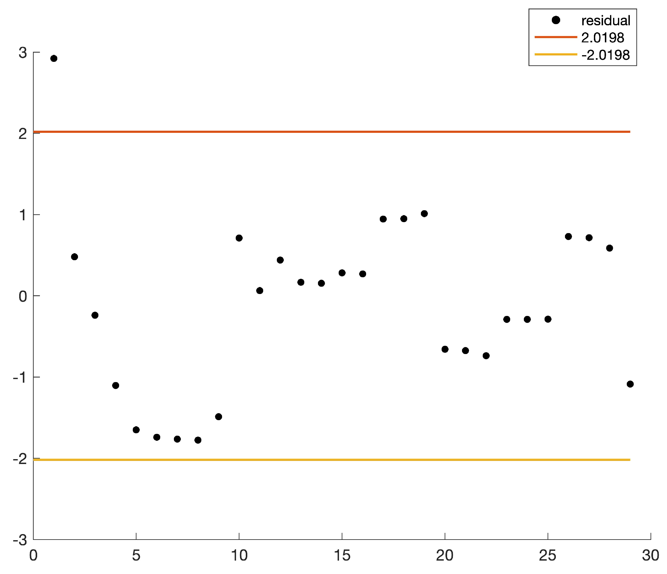
4. Parameter Estimation

How to estimate the unknown parameters of uncertain RL circuit equation based on observed data is a core problem in practice. In this section, we will apply the method of moments to estimating the unknown parameters.

Consider the uncertain RL circuit Equation (1)

$$\mathrm{d}{I}_t=\left(\frac{F\left(t\right)}{l}-\frac{r}{l}{I}_t\right)\mathrm{d}t+\frac{{\sigma }_1}{l}\mathrm{d}{C}_{1t}-\frac{{\sigma }_2}{l}{I}_t\mathrm{d}{C}_{2t}.$$

Suppose that $F\left(t\right)$ is a continuous functions on ℜ, r, l, ${\sigma }_1>0$ and ${\sigma }_2>0$ are unknown parameters to be estimated. Ye [28] suggested that we should consider the difference form of uncertain RL circuit Equation (1), which can be written as

$$\begin{array}{c}\hfill I_{t_{j+1}}-I_{t_j}=\left(\frac{F\left(t_j\right)}{l}-\frac{r}{l}{I}_{t_j}\right)(t_{j+1}-t_j)+\frac{{\sigma }_1}{l}(C_{1t_{j+1}}-C_{1t_j})-\frac{{\sigma }_2}{l}{I}_{t_j}(C_{2t_{j+1}}-C_{2t_j}),\end{array}$$

i.e.,

$$\begin{array}{c}\hfill l{I}_{t_{j+1}}-l{I}_{t_j}+\left(r{I}_{t_j}-F\left(t_j\right)\right)(t_{j+1}-t_j)={\sigma }_1(C_{1t_{j+1}}-C_{1t_j})-{\sigma }_2{I}_{t_j}(C_{2t_{j+1}}-C_{2t_j}).\end{array}$$

Dividing both sides of the above equation by

$$\left({\sigma }_1+{\sigma }_2\left|I_{t_j}\right|\right)(t_{j+1}-t_j),$$

we obtain

$$\begin{array}{c}\hfill \frac{l{I}_{t_{j+1}}-l{I}_{t_j}+\left(r{I}_{t_j}-F\left(t_j\right)\right)(t_{j+1}-t_j)}{\left({\sigma }_1+{\sigma }_2\left|I_{t_j}\right|\right)(t_{j+1}-t_j)}=\frac{{\sigma }_1(C_{1t_{j+1}}-C_{1t_j})-{\sigma }_2{I}_{t_j}(C_{2t_{j+1}}-C_{2t_j})}{\left({\sigma }_1+{\sigma }_2\left|I_{t_j}\right|\right)(t_{j+1}-t_j)}.\end{array}$$

(8)

Suppose that there are n observed data $i_{t_1},i_{t_2},\cdots ,i_{t_n}$ of the solution $I_t$ at time-points $t_1<t_2<\cdots <t_n$. By substituting the observed data into Equation (8), we write

$$h_j(r,l,{\sigma }_1,{\sigma }_2)=\frac{l{i}_{t_{j+1}}-l{i}_{t_j}+\left(r{i}_{t_j}-F\left(t_j\right)\right)(t_{j+1}-t_j)}{\left({\sigma }_1+{\sigma }_2\left|i_{t_j}\right|\right)(t_{j+1}-t_j)}$$

(9)

and

$${\xi }_j=\frac{{\sigma }_1(C_{1t_{j+1}}-C_{1t_j})-{\sigma }_2{i}_{t_j}(C_{2t_{j+1}}-C_{2t_j})}{\left({\sigma }_1+{\sigma }_2\left|i_{t_j}\right|\right)(t_{j+1}-t_j)}$$

(10)

for $j=1,2,\cdots ,n-1$. It is easy to infer that $h_j(r,l,{\sigma }_1,{\sigma }_2)$ can be regarded as a sample of ${\xi }_j$ with $1\le j\le n-1$. On the other hand, it follows from the definition of Liu process and $C_{1t}$ and $C_{2t}$ are two independent Liu processes that

$$\begin{array}{c}\hfill {\xi }_j\sim \frac{\mathcal{N}(0,\left({\sigma }_1+{\sigma }_2\left|i_{t_j}\right|\right)(t_{j+1}-t_j))}{\left({\sigma }_1+{\sigma }_2\left|i_{t_j}\right|\right)(t_{j+1}-t_j)}=\mathcal{N}(0,1)\end{array}$$

for $j=1,2,\cdots ,n-1$. Thus, $h_j(r,l,{\sigma }_1,{\sigma }_2)$, $j=1,2,\cdots ,n-1$ can be regarded as $n-1$ samples of the standard normal uncertainty distribution $\mathcal{N}(0,1)$. For the purpose of estimating the unknown parameters, Yao and Liu [14] suggested that we should equate the first 4 sample moments to the corresponding first 4 population moments. Then, we can get the following system of equations:

$$\begin{array}{c}\hfill \left\{\begin{array}{cc}& {\displaystyle \frac{1}{n-1}\sum _{j=1}^{n-1}{h}_j(r,l,{\sigma }_1,{\sigma }_2)=0}\\ & {\displaystyle \frac{1}{n-1}\sum _{j=1}^{n-1}{\left(h_j(r,l,{\sigma }_1,{\sigma }_2)\right)}^2=1}\\ & {\displaystyle \frac{1}{n-1}\sum _{j=1}^{n-1}{\left(h_j(r,l,{\sigma }_1,{\sigma }_2)\right)}^3=0}\\ & {\displaystyle \frac{1}{n-1}\sum _{j=1}^{n-1}{\left(h_j(r,l,{\sigma }_1,{\sigma }_2)\right)}^4=\frac{21}{5}.}\end{array}\right.\end{array}$$

(11)

The solution $(r^{*},l^{*},{\sigma }_1^{*},{\sigma }_2^{*})$ of the above system of equations is the estimate of unknown parameters, which is called the moment estimate of uncertain RL circuit Equation (1).

Next, we will provide an example to illustrate the moment estimate of uncertain RL circuit equation.

Example 4.

Suppose the potential source provided to the series RL circuit is 5 V, and Simulink (MATLAB R2021a, 9.10.0.1602886, maci64, Simulink, 10.3.) has provided a credible collection of current through the circuit as shown in

Table 1. Observations of a simple series RL circuit in Example 4.

$t_j$ (s)	0.1615	0.3615	0.5615	0.7615	1.0000	1.1924	1.3924	1.5924
$i_{t_j}$ (A)	0.7248	1.4743	2.0879	2.5903	3.0718	3.3696	3.6241	3.8324
$t_j$ (s)	1.7924	2.0381	2.2283	2.6283	2.8283	3.2000	3.6000	3.8000
$i_{t_j}$ (A)	4.0030	4.1827	4.3398	4.5869	4.6780	4.8058	4.8994	4.9338
$t_j$ (s)	4.0000	4.4000	4.8000	5.0000	5.4000	5.8000	6.0000	6.4000
$i_{t_j}$ (A)	4.9621	5.0462	5.1027	5.1234	5.0635	5.0234	5.0086	5.0090
$t_j$ (s)	6.8000	7.0000	7.2000	7.4000	8.0000	9.2000
$i_{t_j}$ (A)	5.0092	5.0093	5.0376	5.0608	5.1080	4.8716

. Since the potential source is constant at 5 V, we have

$$\begin{array}{c}\hfill h_j(r,l,{\sigma }_1,{\sigma }_2)=\frac{l{i}_{t_{j+1}}-l{i}_{t_j}+\left(r{i}_{t_j}-5\right)(t_{j+1}-t_j)}{\left({\sigma }_1+{\sigma }_2\left|i_{t_j}\right|\right)(t_{j+1}-t_j)}\end{array}$$

(12)

for$j=1,2,\cdots ,29$. By solving the system of Equation (11), we have

$$r^{*}=0.9888,l^{*}=1.1621,{\sigma }_1^{*}=0.0015,{\sigma }_2^{*}=0.0318.$$

Therefore, the uncertain RL circuit equation is

$$\begin{array}{c}\hfill \mathrm{d}{I}_t=\left(4.3024-0.8508I_t\right)\mathrm{d}t+0.0013\mathrm{d}{C}_{1t}-0.0274I_t\mathrm{d}{C}_{2t}.\end{array}$$

(13)

Next, we test whether the estimates of unknown parameters are appropriate. By substituting the estimates into (12), we can get 29 residuals ${\epsilon }_1,{\epsilon }_2,\cdots ,{\epsilon }_{29}$ of uncertain RL circuit Equation (13) as shown in

Table 2. Residual plot in Example 4.

j	1	2	3	4	5	6	7	8
${\epsilon }_j$	2.9205	0.4789	−0.2392	−1.1031	−1.6516	−1.7423	−1.7655	−1.7768
j	9	10	11	12	13	14	15	16
${\epsilon }_j$	−1.4899	0.7102	0.0640	0.4388	0.1662	0.1536	0.2809	0.2700
j	17	18	19	20	21	22	23	24
${\epsilon }_j$	0.9452	0.9479	1.0107	−0.6577	−0.6759	−0.7379	−0.2892	−0.2904
j	25	26	27	28	29
${\epsilon }_j$	−0.2891	0.7299	0.7156	0.5866	−1.0873

. Since we have regarded $h_1(r,l,{\sigma }_1,{\sigma }_2),h_2(r,l,{\sigma }_1,{\sigma }_2),$ $\cdots ,h_{29}(r,l,{\sigma }_1,{\sigma }_2)$ as samples of the population $\mathcal{N}(0,1)$, then if the estimates are appropriate, the residuals should be samples of $\mathcal{N}(0,1)$.

Suppose that the residuals are samples of $\mathcal{N}(e,\sigma )$. Then, we consider the following hypotheses:

$$\begin{array}{c}\hfill H_0:e=0 \mathrm{and} \sigma =1 \mathrm{versus} H_1:e\ne 0 \mathrm{or} \sigma \ne 1.\end{array}$$

(14)

For the level of significance $\alpha =0.05$, it follows from uncertain hypothesis test (Ye and Liu [29]) that the test for the hypotheses (14) is

$$\begin{array}{cc}\hfill W=\{& \hfill (z_1,z_2,\cdots ,z_{29}):\mathrm{there} \mathrm{is} \mathrm{at} \mathrm{least}2\mathrm{of} \mathrm{indexes}{j}^{\prime }s \mathrm{with}1\le j\le 29\hfill \\ \hfill & \hfill \mathrm{such} \mathrm{that}{z}_j<-2.0198\mathrm{or}{z}_j>2.0198\}.\hfill \end{array}$$

As shown in Figure 5, we can see that only

$${\epsilon }_1\notin [-2.0198,2.0198].$$

Thus, $({\epsilon }_1,{\epsilon }_2,\cdots ,{\epsilon }_{29})\notin W$ and then we think the estimated parameters $(r^{*},l^{*},{\sigma }_1^{*},{\sigma }_2^{*})$ is appropriate.

In addition, if we divide the residuals into two groups to test whether ${\epsilon }_1,{\epsilon }_2,\cdots ,{\epsilon }_9$ and ${\epsilon }_{10},{\epsilon }_{11},\cdots ,{\epsilon }_{29}$ are from the same population, then the result of the two-sample Kolmogorov–Smirnov test is to reject the hypothesis that they are from the same population with a significance level $\alpha =0.05$, and the p-value is $0.0038$. That is, the residuals are not identically distributed in the sense of probability theory. Therefore, we should regard the residuals as uncertain variables and use uncertain differential equation to model the circuit system.

5. Conclusions

By considering the external noise and internal noise, this paper first applied a multifactor uncertain differential equation to modeling the time evolution of a simple series RL electrical circuit system. Based on the uncertain RL circuit equation, some results were obtained, such as the solution of uncertain RL circuit equation, the inverse uncertainty distribution of solution and the applications of solution. Furthermore, parameter estimation for the uncertain RL circuit equation was also considered.

6. Future Work

Further research may consider modeling more complex circuit systems such as RLC circuit systems, delay circuit systems, and circuit networks.

References

1. Liu, B. Uncertainty Theory, 2nd ed.; Springer: Berlin, Germany, 2007. [Google Scholar]
2. Liu, B. Some research problems in uncertainty theory. J. Uncertain Syst. 2009, 3, 3–10. [Google Scholar]
3. Liu, B. Fuzzy process, hybrid process and uncertain process. J. Uncertain Syst. 2008, 2, 3–16. [Google Scholar]
4. Chen, X.; Liu, B. Existence and uniqueness theorem for uncertain differential equations. Fuzzy Optim. Decis. Ma. 2010, 9, 69–81. [Google Scholar]
5. Gao, Y. Existence and uniqueness theorem on uncertain differential equations with local Lipschitz condition. J. Uncertain Syst. 2012, 6, 223–232. [Google Scholar]
6. Yao, K.; Gao, J.; Gao, Y. Some stability theorems of uncertain differential equation. Fuzzy Optim. Decis. Ma. 2013, 12, 3–13. [Google Scholar] [CrossRef]
7. Sheng, Y.; Wang, C. Stability in the p-th moment for uncertain differential equation. J. Intell. Fuzzy Syst. 2014, 26, 1263–1271. [Google Scholar] [CrossRef]
8. Yao, K.; Ke, H.; Sheng, Y. Stability in mean for uncertain differential equation. Fuzzy Optim. Decis. Ma. 2015, 14, 365–379. [Google Scholar] [CrossRef]
9. Yang, X.; Ni, Y.; Zhang, Y. Stability in inverse distribution for uncertain differential equations. J. Intell. Fuzzy Syst. 2017, 32, 2051–2059. [Google Scholar] [CrossRef] [Green Version]
10. Yao, K.; Chen, X. A numerical method for solving uncertain differential equations. J. Intell. Fuzzy Syst. 2013, 25, 825–832. [Google Scholar] [CrossRef]
11. Yang, X.; Shen, Y. Runge-Kutta method for solving uncertain differential equations. J. Uncertain. Anal. Appl. 2015, 3, 17. [Google Scholar] [CrossRef] [Green Version]
12. Yang, X.; Ralescu, D. Adams method for solving uncertain differential equations. Appl. Math. Comput. 2015, 270, 993–1003. [Google Scholar] [CrossRef]
13. Gao, R. Milne method for solving uncertain differential equations. Appl. Math. Comput. 2016, 274, 774–785. [Google Scholar]
14. Yao, K.; Liu, B. Parameter estimation in uncertain differential equations. Fuzzy Optim. Decis. Ma. 2020, 19, 1–12. [Google Scholar] [CrossRef]
15. Liu, Z. Generalized moment estimation for uncertain differential equations. Appl. Math. Comput. 2021, 392, 125724. [Google Scholar] [CrossRef]
16. Yang, X.; Liu, Y.; Park, G. Parameter estimation of uncertain differential equation with application to financial market. Chaos Solitons Fract. 2020, 139, 110026. [Google Scholar] [CrossRef]
17. Sheng, Y.; Yao, K.; Chen, X. Least squares estimation in uncertain differential equations. IEEE Trans. Fuzzy Syst. 2020, 28, 2651–2655. [Google Scholar] [CrossRef]
18. Liu, Y.; Liu, B. Estimating Unknown Parameters in Uncertain Differential Equation by Maximum Likelihood Estimation. 2020. submitted. [Google Scholar]
19. Lio, W.; Liu, B. Initial value estimation of uncertain differential equations and zero-day of COVID-19 spread in China. Fuzzy Optim. Decis. Ma. 2021, 20, 177–188. [Google Scholar]
20. Chen, X.; Li, J.; Xiao, C.; Yang, P. Numerical solution and parameter estimation for uncertain SIR model with application to COVID-19. Fuzzy Optim. Decis. Ma. 2021, 20, 189–208. [Google Scholar]
21. Jia, L.; Chen, W. Uncertain SEIAR model for COVID-19 cases in China. Fuzzy Optim. Decis. Mak. 2021, 20, 243–259. [Google Scholar] [CrossRef]
22. Bennett, W. Electrical Noise; McGraw-Hill: New York, NY, USA, 1960. [Google Scholar]
23. Kampowsky, W.; Rentrop, P.; Schmidt, W. Classification and numerical simulation of electric circuits. Sur. Math. Ind. 1992, 2, 23–65. [Google Scholar]
24. Penski, C. A new numerical method for SDEs and its application in circuit simulation. J. Comput. Appl. Math. 2000, 115, 461–470. [Google Scholar] [CrossRef] [Green Version]
25. Kolarova, E. Modelling RL electrical circuits by stochastic differential equations. In Proceedings of the The International Conference on “Computer as a Tool”, Belgrade, Serbia, 21–24 November 2005; pp. 1236–1238. [Google Scholar]
26. Kolarova, E. An application of stochastic integral equations to electrical networks. Acta Electrotech. Inform. 2008, 8, 14–17. [Google Scholar]
27. Liu, Y. Uncertain circuit equation. J. Uncertain Syst. 2021, 14, 2150018. [Google Scholar] [CrossRef]
28. Ye, T. Parameter Estimation in Multifactor Uncertain Differential Equation with Application to Stock Market; Technical Report; 2021. [Google Scholar]
29. Ye, T.; Liu, B. Uncertain hypothesis test with application to uncertain regression analysis. Fuzzy Optim. Decis. Mak. 2021. [Google Scholar] [CrossRef]
Figure 1. Inverse uncertainty distribution of solution with I 0 = 0 , r = 5 and l = 10 in Example 1.
Symmetry 13 02103 g001
Figure 2. Inverse uncertainty distribution of solution with I 0 = 0 , r = 5 and l = 10 in Example 2.
Symmetry 13 02103 g002
Figure 3. Inverse uncertainty distribution of the maximum current with α ( 0 , 0.8 ] , I 0 = 0 , r = 5 and l = 10 in Example 3.
Symmetry 13 02103 g003
Figure 4. Inverse uncertainty distribution of the amount of charge passing through the resistor with I 0 = 0 , r = 5 and l = 10 in Example 3.
Symmetry 13 02103 g004
Figure 5. Residual plot in Example 4.
Symmetry 13 02103 g005