Article

PQMLE of a Partially Linear Varying Coefficient Spatial Autoregressive Panel Model with Random Effects

1
College of Mathematics and Statistics, Fujian Normal University, Fuzhou 350117, China
2
School of Computer Science and Mathematics, Fujian University of Technology, Fuzhou 350118, China
*
Author to whom correspondence should be addressed.
Symmetry 2021, 13(11), 2057; https://doi.org/10.3390/sym13112057
Submission received: 26 September 2021 / Revised: 15 October 2021 / Accepted: 19 October 2021 / Published: 1 November 2021
(This article belongs to the Special Issue Probability, Statistics and Applied Mathematics)

Abstract

:
This article deals with asymmetrical spatial data which can be modeled by a partially linear varying coefficient spatial autoregressive panel model (PLVCSARPM) with random effects. We constructed its profile quasi-maximum likelihood estimators (PQMLE). The consistency and asymptotic normality of the estimators were proved under some regular conditions. Monte Carlo simulations implied our estimators have good finite sample performance. Finally, a set of asymmetric real data applications was analyzed for illustrating the performance of the provided method.

1. Introduction

Spatial regression models are used to deal with spatially dependent data which widely exist in many fields, such as economics, environmental science and geography. According to the different types of spatial interaction effects, spatial regression models can be sorted into three basic categories (see [1]). The first category is spatial autoregressive (SAR) models, which include endogenous interaction effects among observations of response variables at different spatial scales (see [2]). The second category is spatial durbin models (SDM), which include exogenous interaction effects among observations of covariates and endogenous interaction effects among observations of response variables at different spatial scales (see [3,4]). The third category is spatial error models (SEM), which include interaction effects among disturbance terms of different spatial scales (see [5]). Among them, the SAR models proposed by [6] may be the most popular. The developments in the testing and estimation of SAR models for sectional data were summarized in the books by [7,8,9] and the surveys by [10,11,12,13,14,15,16], among others. Compared to sectional data models, panel data models exhibit an excellent capacity for capturing the complex situations by using abundant datasets built up over time and adding individual-specific or time-specific fixed or random effects. Their theories, methods and applications can be found in the books by [17,18,19,20] and the surveys by [21,22,23,24,25,26], among others.
The above mentioned research literature mainly focuses on linear parametric models. Although the estimations and properties of these models have been well established, they are often unrealistic in application, for the reason that they are unable to accommodate sufficient flexibility to accommodate complex structures (e.g., nonlinearity). Moreover, mis-specification of the data generation mechanism by a linear parametric model could lead to excessive modeling biases or even erroneous conclusions.
Ref. [27] pointed out that the relationship between variables in space usually exhibits highly complexity in reality. Therefore, researches have proposed a number of solution methods. In video coding systems, transmission problems are usually dealt with wavelet-based methods. Ref. [28] proposed a low-band-shift method which avoids the shift-variant property of the wavelet transform and performs the motion compensation more precisely and efficiently. Ref. [29] obtained a wavelet-based lossless video coding scheme that switches between two operations based on the different amount of motion activities between two consecutive frames. More theories and applications can be found in [30,31,32]. In econometrics, some nonparametric and semiparametric spatial regression models have been developed to relax the linear parametric model settings. For sectional spatial data, ref. [33] studied the GMM estimation of a nonparametric SAR model; Ref. [34] investigated the PQMLE of a partially linear nonparametric SAR model. However, such nonparametric SAR models may cause the “curse of dimensionality” when the dimension of covariates is higher. In order to overcome this drawback, ref. [35] studied two-step SGMM estimators and their asymptotic properties for spatial models with space-varying coefficients. Ref. [36] proposed a semiparametric series-based least squares estimating procedure for a semiparametric varying coefficient mixed regressive SAR model and derived the asymptotical normality of the estimators. Some other related research works can be found in [37,38,39,40,41,42]. For panel spatial data, ref. [43] obtained PMLE and its asymptotical normality of varying the coefficient SAR panel model with random effects; Ref. [44] applied instrumental variable estimation to a semiparametric varying coefficient spatial panel data model with random effects and the investigated asymptotical normality of the estimators.
In this paper, we extend the varying coefficient spatial panel model with random effects given in [43] to a PLVCSARPM with random effects. By adding a linear part to the model of [43], we can simultaneously capture linearity, non-linearity and the spatial correlation relationships of exogenous variables in a response variable. By using the profile quasimaximum likelihood method to estimate PLVCSARPM with random effects, we proved the consistency and asymptotic normality of the estimators under some regular conditions. Monte Carlo simulations and real data analysis show that our estimators perform well.
This paper is organized as follows: Section 2 introduces the PLVCSARPM with random effects and constructs its PQMLE. Section 3 proves the asymptotic properties of estimators. Section 4 presents the small sample estimates using Monte Carlo simulations. Section 5 analyzes a set of asymmetric real data applications for illustrating the performance of the proposed method. A summary is given in Section 6. The proofs of some important theorems and lemmas are given in Appendix A.

2. The Model and Estimators

Consider the following partially linear varying coefficient spatial autoregressive panel model (PLVCSARPM) with random effects:
y i t = ρ ( W 0 Y t ) i + x i t β ( u i t ) + z i t α + b i + ε i t , 1 i N , 1 t T ,
where i refers to a spatial unit; t refers to a given time period; y i t are observations of a response variable; Y t = ( y 1 t , y 2 t , , y N t ) ; x i t = ( x i t 1 , x i t 2 , , x i t p ) and z i t = ( z i t 1 , z i t 2 , , z i t q ) are observations of p-dimensional and q-dimensional covariates, respectively; β ( u i t ) = ( β 1 ( u i t ) , β 2 ( u i t ) , , β p ( u i t ) ) is an unknown univariate varying coefficient function vector; β s ( u ) ( s = 1 , 2 , , p ) are unknown smoothing functions of u; ρ ( | ρ | < 1 ) is an unknown spatial correlation coefficient; α = ( α 1 , α 2 , , α q ) is a regression coefficient vector of z i t ; W 0 is an N × N predetermined spatial weight matrix; ( W 0 Y t ) i is the ith component of W 0 Y t ; ε i t are i.i.d. error terms with zero means and variance σ ε 2 ; b i are i.i.d. variables with zero means and variance σ b 2 , ε i t are independent of b i . Let θ 0 = ( ρ 0 , α 0 , σ b 0 2 , σ ε 0 2 ) be the true parameter vector of θ = ( ρ , α , σ b 2 , σ ε 2 ) and β 0 ( u i t ) be the true varying coefficient function of β ( u i t ) .
The model (1) can be simplified as the following matrix form:
Y = ρ W Y + X β ( u ) + Z α + U b + ε ,
where Y = ( y 11 , y 12 , , y N T ) ; X = ( x 11 , x 12 , , x N T ) ; Z = ( z 11 , z 12 , , z N T ) ; ε = ( ε 11 , ε 12 , , ε N T ) ; W = W 0 I T ; b = ( b 1 , b 2 , , b N ) ; U = I N e T ; I N is an N × N identity matrix; I T is a T × T identity matrix; ⊗ denotes the Kronecker product; e T is a T × 1 vector consisting of 1.
Define A ( ρ ) = I ρ W ; then the model (2) can be rewritten as:
A ( ρ ) Y = X β ( u ) + Z α + U b + ε ,
where I is an N T × N T unit matrix. For the model (3), it is easy to get the following facts:
( U b + ε ) / ( Y ) = A ( ρ ) , Σ = V a r ( U b + ε ) = σ ε 2 I + σ b 2 I N ( e T e T ) ,
| Σ | = σ ε 2 N ( T 1 ) ( σ b 2 + T σ ε 2 ) N , Σ 1 = 1 σ ε 2 I + ( 1 σ ε 2 + T σ b 2 1 T σ b 2 ) I N ( 1 T e T e T ) .
According to [12], the quasi-log-likelihood function of the model (3) can be written as follows:
l n L ( θ ) = N ( T 1 ) 2 l n σ ε 2 N 2 l n ( σ ε 2 + T σ b 2 ) 1 2 ( σ ε 2 + T σ b 2 ) [ A ( ρ ) Y X β ( u ) Z α ] H [ A ( ρ ) Y X β ( u ) Z α ] 1 2 σ ε 2 [ A ( ρ ) Y X β ( u ) Z α ] ( I H ) [ A ( ρ ) Y X β ( u ) Z α ] + l n | A ( ρ ) | + c ,
where H = I N ( T 1 e T e T ) , and c is a constant.
By maximizing the above quasi-log-likelihood function with respect to θ , the quasi-maximum likelihood estimators of α , σ b 2 and σ ε 2 can be easily obtained as
α ˜ = [ Z ( I S ) ( H σ ε 2 + T σ b 2 + I H σ ε 2 ) ( I S ) Z ] 1 Z ( I S ) ( H σ ε 2 + T σ b 2 + I H σ ε 2 ) A ( ρ ) Y ,
σ ˜ ε 2 = [ N ( T 1 ) ] 1 [ A ( ρ ) Y X β ( u ) Z α ] ( I H ) [ A ( ρ ) Y X β ( u ) Z α ] ,
σ ˜ b 2 = ( N T ) 1 [ A ( ρ ) Y X β ( u ) Z α ] H [ A ( ρ ) Y X β ( u ) Z α ] T 1 σ ˜ ε 2 .
By substituting (5)–(7) into (4), we have the concentrated quasi-log-likelihood function of ρ as
l n L ( ρ ) = N ( T 1 ) 2 l n σ ˜ ε 2 N 2 l n ( σ ˜ ε 2 + T σ ˜ b 2 ) N T 2 + l n | A ( ρ ) | .
It is obvious that we cannot directly obtain the quasi-maximum likelihood estimator of ρ by maximizing the above formula because β ( u i t ) is an unknown function. In order to overcome this problem, we use the PQMLE method and working independence theory ([45,46]) to estimate the unknown parameters and varying coefficient functions of the model (1).
The main steps are as follows:
Step 1 Suppose that θ is known. β s ( · ) can be approximated by the first-order Taylor expansion
β s ( u i t ) β s ( u ) + ( u i t u ) β ˙ s ( u ) = ^ a 1 s + a 2 s ( u i t u ) , s = 1 , 2 , , p
for u i t in a neighborhood of u, where a 2 s is the first order derivative of β ( u ) . Let a 1 = ( a 11 , a 12 , , a 1 p ) and a 2 = ( a 21 , a 22 , , a 2 p ) ; then estimators of a 1 and a 2 can be obtained by
( a ^ 1 , a ^ 2 ) = arg min a 1 , a 2 1 N T i = 1 N t = 1 T [ y ˜ i t s = 1 p ( a 1 s + a 2 s ( u i t u ) ) x i t s ] 2 K h ( u i t u ) ,
where y ˜ i t = y i t ρ ( W 0 Y t ) i z i t α , K h ( u i t u ) = h 1 K ( ( u i t u ) / h ) , K ( · ) is a kernel function and h is the bandwidth. Therefore, the feasible initial estimator of β ( u ) can be obtained by β ^ I N ( u ) = a ^ 1 = ( a ^ 11 , a ^ 12 , , a ^ 1 p ) .
Denote W u = d i a g ( K h ( u 11 u ) , K h ( u 12 u ) , , K h ( u N T u ) ) , Y ˜   =   ( y ˜ 11 , y ˜ 12 , , y ˜ N T ) , δ = ( a 11 , , a 1 p , h a 21 , , h a 2 p ) and D u = x 11 x N T u 11 u h x 11 u N T u h x N T , then we have
δ ^ = arg min δ 1 N T ( Y ˜ D u δ ) W u ( Y ˜ D u δ ) .
Therefore, we obtain
δ ^ = ( D u W u D u ) 1 D u W u Y ˜ .
Let S u = 1 N T D u W u D u , T u = 1 N T D u W u Y ˜ and e 0 = ( I p , 0 p ) . It is easy to know that
β ^ I N ( u ) = ( a ^ 11 , a ^ 12 , , a ^ 1 p ) = e 0 S u 1 T u ,
where e 0 S u = s ( u ) . Consequently, the initial estimator of X β ( u ) is given by
X β ^ I N ( u ) = ( x 11 0 ) ( D u 11 W u 11 D u 11 ) 1 D u 11 W u 11 ( x 12 0 ) ( D u 12 W u 12 D u 12 ) 1 D u 12 W u 12 ( x N T 0 ) ( D u N T W u N T D u N T ) 1 D u N T W u N T Y ˜ = ^ S Y ˜ ,
where
S = ( x 11 0 ) ( D u 11 W u 11 D u 11 ) 1 D u 11 W u 11 ( x 12 0 ) ( D u 12 W u 12 D u 12 ) 1 D u 12 W u 12 ( x N T 0 ) ( D u N T W u N T D u N T ) 1 D u N T W u N T .
Step 2 Replacing β ( u ) of (4) with β ^ I N ( u ) , the estimator θ ^ of θ can be obtained by maximizing approximate quasi-log-likelihood function:
l n L ^ ( θ ) = N ( T 1 ) 2 l n σ ε 2 1 2 ( σ ε 2 + T σ b 2 ) [ A ( ρ ) Y Z α ] ( I S ) H ( I S ) [ A ( ρ ) Y Z α ] N 2 l n ( σ ε 2 + T σ b 2 ) 1 2 σ ε 2 [ A ( ρ ) Y Z α ] ( I S ) ( I H ) ( I S ) [ A ( ρ ) Y Z α ] + l n | A ( ρ ) | + c .
In the real estimation of θ , the procedure is realized by following steps:
Firstly, assume ρ is known. The initial estimators of σ b 2 , σ ε 2 and α are obtained by maximizing (9). Then, we find
σ ^ ε I N 2 = [ N ( T 1 ) ] 1 [ Y ˜ X β ^ I N ( u ) ] ( I H ) [ Y ˜ X β ^ I N ( u ) ] ,
σ ^ b I N 2 = ( N T ) 1 [ Y ˜ X β ^ I N ( u ) ] H [ Y ˜ X β ^ I N ( u ) ] T 1 σ ^ ε I N 2 ,
α ^ I N = [ Z ( I S ) ( H σ ^ ε I N 2 + T σ ^ b I N 2 + I H σ ^ ε I N 2 ) ( I S ) Z ] 1 Z ( I S ) ( H σ ^ ε I N 2 + T σ ^ b I N 2 + I H σ ^ ε I N 2 ) A ( ρ ) Y .
Secondly, with the estimated σ ^ ε I N 2 , σ ^ b I N 2 and α ^ I N , update ρ ^ by maximizing the concentrated quasi-log-likelihood function of ρ :
l n L ˜ ( ρ ) = N ( T 1 ) 2 l n σ ^ ε I N 2 N 2 l n ( σ ^ ε I N 2 + T σ ^ b I N 2 ) + l n | A ( ρ ) | + c .
Therefore, the estimator of ρ is obtained by:
ρ ^ = arg max ρ l n L ˜ ( ρ ) .
Step 3 By substituting ρ ^ into (10), (11) and (12), respectively, the final estimators of σ b 2 , σ ε 2 and α are computed as follows:
σ ^ ε 2 = [ N ( T 1 ) ] 1 Y ˜ ^ ( I S ) ( I H ) ( I S ) Y ˜ ^ ,
σ ^ b 2 = ( N T ) 1 Y ˜ ^ ( I S ) H ( I S ) Y ˜ ^ T 1 σ ^ ε 2 ,
α ^ = [ Z ( I S ) ( H σ ^ ε 2 + T σ ^ b 2 + I H σ ^ ε 2 ) ( I S ) Z ] 1 Z ( I S ) ( H σ ^ ε 2 + T σ ^ b 2 + I H σ ^ ε 2 ) A ( ρ ^ ) Y .
Step 4 By replacing ρ with ρ ^ in (8), we get the ultimate estimator of β ( u ) :
β ^ ( u ) = e 0 [ D u W u D u ] 1 D u W u Y ˜ ^ .
where Y ˜ ^ = A ( ρ ^ ) Y Z α ^ , A ( ρ ^ ) = I ρ ^ W .

3. Asymptotic Properties for the Estimators

In this section, we focus on studying consistency and asymptotic normality of the PQMLEs given in Section 2. To prove these asymptotic properties, we need the following assumptions to hold.
To provide a rigorous analysis, we make the following assumptions.
Assumption 1.
(i)
ε i t and b i are uncorrelated to x i t and z i t , and satisfy E ( b i | x i t , z i t ) = 0 , V a r ( b i | x i t , z i t ) = σ b 2 < , E ( b i x i t ) < , E ( b i z i t ) < , E ( ε i | x i t , z i t ) = 0 , E ( ε i x i t ) < , V a r ( ε i | x i t , z i t ) = σ ε 2 < and E ( ε i z i t ) < , where · represents the Euclidean norm. Moreover, E ( | ε | r ) < and E ( | b | r ) < for some r > 4 .
(ii)
{ ( u i t , ε i t ) } i = 1 , t = 1 N , T are i . i . d random sequences. The density function f t ( u ) of u i t is non-zero, uniformly bounded and second-order continuously differentiable on U , where U is the supporting set of K ( u ) . Ω 11 ( u ) = E ( x i t x i t | u i t = u ) < exists, and it has a second-order continuous derivative; Ω 12 ( u ) = E ( x i t z i t | u i t = u ) and Ω 22 ( u ) = E ( z i t z i t | u i t = u ) are second-order continuously differentiable on U ; E ( x i t x i s | u i t = u ) = 0 , E ( z i t z i s | u i t = u ) = 0 and E ( x i t z i s | u i t = u ) = 0 for t s ; E ( x i t x i t | u i t = u ) 0 , E ( x i t ε i t | u i t ) = 0 and E ( x i t b i t | u i t ) = 0 .
(iii)
Real valued function β s ( u ) ( s = 1 , 2 , , p ) is second-order, continuously differentiable and satisfies the first order Lipschitz condition, | x i t β s ( u ) | m β at any u, | z i t α | m α , where m β and m α are positive and constant.
(iv)
{ x i t , z i t } i = 1 , t = 1 N , T are i.i.d. random variables from the population. Moreover, max i , t E ( | x i t | r ) < and max i , t E ( | z i t | r ) < for r 4 .
Assumption 2.
(i)
As a normalization, the diagonal elements ϖ i i of W 0 are 0 for all i and ϖ i j are at most of order l N 1 , denoted by O ( 1 / l N ) .
(ii)
The ratio l N / N 0 as N goes to infinity.
(iii)
A ( ρ ) is nonsingular for any | ρ | < 1 .
(iv)
The matrices W 0 and A 1 ( ρ ) are uniformly bounded in both row and column sums in absolute value.
Assumption 3.
K ( · ) is a nonnegative continuous even function. Let μ l = k ( υ ) υ l d υ , υ l = k 2 ( υ ) υ l d υ ; then μ l = υ l = 0 for any positive odd number. Meanwhile, μ 0 = 1 , μ 2 0 .
Assumption 4.
If N , T and h 0 , then N T h .
Assumption 5.
There is an unique θ 0 to make the model (1) tenable.
Assumption 6.
ϕ Q 0 Z ϕ Z Z 1 ϕ Q 0 Z + ϕ Q 0 Q 0 0 , where
ϕ Q 0 Z = l i m N l i m T 1 N T Q 0 ( I S ) ( I S ) Z , ϕ Z Z = l i m N l i m T 1 N T Z ( I S ) ( I S ) Z ,
ϕ Q 0 Q 0 = l i m N l i m T 1 N T Q 0 ( I S ) ( I S ) Q 0 , Q 0 = G 0 ( Z α 0 + X β 0 ) , G 0 = W A 1 ( ρ 0 ) .
Remark 1.
Assumption 1 provides the essential features of the regressors and disturbances for the model (see [47]). Assumption 2 concerns the basic features of the spatial weights matrix and the parallel Assumptions 2–5 of [12]. Assumption 2(i) is always satisfied if l N is a bounded sequence. We allow l N to be divergent, but at a rate smaller than N, as specified in Assumption 2(ii). Assumption 2(iii) guarantees that model (2) has an equilibrium given by (3). Assumption 2(iv) is also assumed in [12], and it limits the spatial correlation to some degree but facilitates the study of the asymptotic properties of the spatial parameter estimators. Assumptions 3 and 4 concern the kernel function and bandwidth sequence. Assumption 5 offers a unique identification condition, and Assumption 6 is necessary for proof of asymptotic normality.
In order to prove large sample properties of estimators, we need introduce the following useful lemmas. Before that, we simplify the model (2) and obtain reduced form equation of Y as follows:
Y = X β 0 ( u ) + Z α 0 + ρ G ( Z α 0 + X β 0 ( u ) ) + A 1 ( ρ 0 ) ( U b + ε ) ,
where A 1 ( ρ 0 ) = I + ρ 0 G 0 ; G 0 = W A 1 ( ρ 0 ) . The above equations are frequently used in a later derivation.
Lemma 1.
Let { ( X 1 , Y 1 ) , ( X 2 , Y 2 ) , , ( X n , Y n ) } be i.i.d. random vectors, where Y i are scalar random variables. Further, assume that E | y | r f ( x , y ) d y < , where f denotes the joint density of ( X , Y ) . Let K be a bounded positive function with a bounded support, satisfying a Lipschitz condition. Given that n 2 τ 1 h for some τ < 1 r 1 ,
s u p x | 1 n i = 1 n [ K h ( X i x ) Y i E K h ( X i x ) Y i ] | = O p ( { l o g ( 1 / h ) n h } 1 / 2 ) .
The proof can be found in [48].
Lemma 2.
Under Assumptions 1–4, we have
S u p F ( u ) Ω 11 ( u ) 0 0 μ 2 Ω 11 ( u ) ,
where F ( u ) = l i m T 1 T i = 1 T f t ( u ) and Ω 11 = E ( x i t x i t | u i t = u ) , i = 1 , 2 , , N , t = 1 , 2 , , T .
Proof See the Appendix A.
Lemma 3.
Under Assumptions 1–4, we have β ^ I N ( u ) p β 0 ( u ) .
Proof See the Appendix A.
Lemma 4.
Under Assumptions 1–4, we have
(i)
1 N T Z ( I S ) ( I H ) ( I S ) Z p Ω 22 ( u ) Ω 11 1 ( u ) Ω 12 ( u ) ;
(ii)
( I S ) X β ( u ) = o p ( 1 ) , ( I S ) Z α = o p ( 1 ) ;
(iii)
( I S ) G X β ( u ) = O p ( 1 ) , ( I S ) G Z α = O p ( 1 ) ;
(iv)
S ( U b + ε ) = o p ( 1 ) , S G ( U b + ε ) = o p ( 1 ) .
The proof can be found in [37].
Lemma 5.
Under Assumptions 1–6, Σ θ 0 = E [ 1 N T 2 l n L ( θ 0 ) θ θ ] is a positive definite matrix and
1 N T 2 l n L ( θ 0 ) θ θ = σ b 2 E [ Q 0 P Q 0 ] N ( σ ε 0 2 + T σ b 0 2 ) σ ε 0 2 + σ b 0 2 [ t r ( G 0 G 0 ) + t r ( G 0 H G 0 ) ] N σ ε 0 2 + t r ( G 0 G 0 ) t r ( G 0 2 ) N T * * * t r ( G 0 H ) N T + ( σ ε 0 2 + T σ b 0 2 ) [ t r ( G 0 ) t r ( G 0 H ) ] N T σ ε 0 4 1 2 σ ε 0 4 * * t r ( G 0 H ) N T ( σ ε 0 2 + T σ b 0 2 ) 1 2 ( σ ε 0 2 + T σ b 0 2 ) 2 T 2 ( σ ε 0 2 + T σ b 0 2 ) 2 * σ b 0 2 E [ Q 0 P Z ] N ( σ ε 0 2 + T σ b 0 2 ) σ ε 0 2 0 0 E [ Z P Z ] N T σ ε 0 2 ( σ ε 0 2 + T σ b 0 2 ) + o p ( 1 ) .
Proof See the Appendix A.
With the above lemmas, we state main results as follows. Their detailed proofs are given in the Appendix A.
Theorem 1.
Under Assumptions 1–5, we have ρ ^ ρ 0 = o p ( 1 ) and α ^ α 0 = o p ( 1 ) .
Theorem 2.
Under Assumptions 1–5, we have β ^ ( u ) β 0 ( u ) = o p ( 1 ) .
Theorem 3.
Under Assumptions 1–5, we have σ ^ ε 2 σ ε 0 2 = o p ( 1 ) and σ ^ b 2 σ b 0 2 = o p ( 1 ) .
Theorem 4.
Under Assumptions 1–6, we have
N T ( θ ^ θ 0 ) D N ( 0 , Σ θ 0 1 + Σ θ 0 1 Ω θ Σ θ 0 1 ) .
where “ D ” represents convergence in distribution, Σ θ 0 = E [ 1 N T 2 l n L ( θ 0 ) θ θ ] is the average Hessian matrix (information matrix when ε and b are normally distributed, respectively), Ω θ = E ( Ω θ N T ) and Ω θ N T = 1 N T l n L ( θ 0 ) θ · 1 N T l n L ( θ 0 ) θ + 1 N T 2 l n L ( θ 0 ) θ θ .
Theorem 5.
Under Assumptions 1–5, we have
N T h ( β ^ ( u ) β 0 ( u ) φ ( u ) ) D N ( 0 , γ 2 ( u ) ) ,
where γ 2 ( u ) and φ ( u ) satisfy φ ( u ) = 1 2 h 2 μ 2 β ¨ ( u ) and γ 2 ( u ) = υ 0 ( σ ε , 0 2 + σ b , 0 2 ) [ F ( u ) Ω 11 ( u ) ] 1 ,   F ( u ) = l i m T 1 T t = 1 T f t ( u ) ,   Ω 11 ( u ) = E ( x i t x i t | u i t = u ) and β ¨ ( u ) is the second-order derivative of β ( u ) , i = 1 , 2 , , N , t = 1 , 2 , , T . Furthermore, if N T h 5 0 , then we have
N T h ( β ^ ( u ) β 0 ( u ) ) D N ( 0 , γ 2 ( u ) ) .

4. Monte Carlo Simulation

In this section, Monte Carlo simulations are presented, which were carried out to investigate the finite sample performance of PQMLEs. The sample standard deviation ( S D ) and two root mean square errors ( R M S E 1 and R M S E 2 ) were used to measure the estimation performance. R M S E 1 and R M S E 2 are defined as:
RMSE 1 = 1 m c n i = 1 m c n ( θ ^ i θ 0 ) 2 1 2 , RMSE 2 = ( θ ^ 0.5 θ 0 ) 2 + θ ^ 0.75 θ ^ 0.25 1.35 ,
where m c n is the number of iterations; θ ^ i ( i = 1 , 2 , , m c n ) are estimates of θ for each iteration, θ 0 is the true value of θ ; θ ^ 0.25 , θ ^ 0.5 and θ ^ 0.75 are the upper quartile, median and lower quartile of parametric estimates, respectively. For the nonparametric estimates, we took the mean absolute deviation error ( M A D E ) as the evaluation criterion:
MADE j = Q 1 q = 1 Q | β ^ j ( u q ) β j ( u q ) | , j = 1 , 2 , , m c n ,
where { u q } q = 1 Q are Q fixed grid points in the support set of u. In the simulations, we applied the rule of thumb method of [48] to choose the optimal width and let kernel function be an Epanechnikov kernel K ( u ) = ( 3 4 5 ) ( 1 1 5 u 2 ) 1 ( u 2 5 ) (see [33]).
We ran a small simulation experiment with m c n = 500 and generated the simulation data from following model:
y i t = ρ ( W 0 Y t ) i + x i t β ( u i t ) + z i t α + b i + ε i t , i = 1 , 2 , , N , t = 1 , 2 , , T ,
where we assume that x i t U [ 2 , 2 ] , z i t U [ 2 , 2 ] , u i t U [ 3 , 3 ] , ε i t i . i . d . N ( 0 , 0.5 ) , b i i . i . d . N ( 0 , 1 ) , β 1 ( u i t ) = 0.5 u i t + s i n ( 1.5 u i t ) , β 2 ( u i t ) = u i t 2 + 0.5 u i t , ( α 1 , α 2 ) = ( 1 , 1.5 ) and ρ = 0.25 , 0.5 and 0.75, respectively. Furthermore, we chose the Rook weight matrix (see [7]) to investigate the influence of the spatial weight matrix on the estimates. Our simulation results for both cases T = 10 and T = 15 are presented in Table 1, Table 2, Table 3, Table 4, Table 5 and Table 6.
By observing the simulation results in Table 1, Table 2, Table 3, Table 4, Table 5 and Table 6, one can obtain the following findings: (1) The R M S E 1 s and R M S E 2 s for ρ ^ , σ ^ ε 2 , α ^ 1 and α ^ 2 were fairly small for almost all cases, and they decreased as N increased. The S D s and R M S E s for σ ^ b 2 are not negligible for small sample sizes, but they decreased as N increased. (2) For fixed T, as N increased, the S D s for ρ ^ , σ ^ ε 2 , σ ^ b 2 , α ^ 1 and α ^ 2 decreased for all cases. R M S E 1 s and R M S E 2 s for α ^ 1 and α ^ 2 decreased rapidly, whereas the R M S E s for estimates of the others parameters did not change much. For fixed N, as T increased, the behavior of the estimates of parameters was similar to the case where N changed under the fixed T. (3) The S D s for M A D E s of varying coefficient functions β 1 ( u ) and β 2 ( u ) decreased as T or N increased. Combined with the above three findings, we conclude that the estimates of the parameter and unknown varying coefficient functions were convergent.
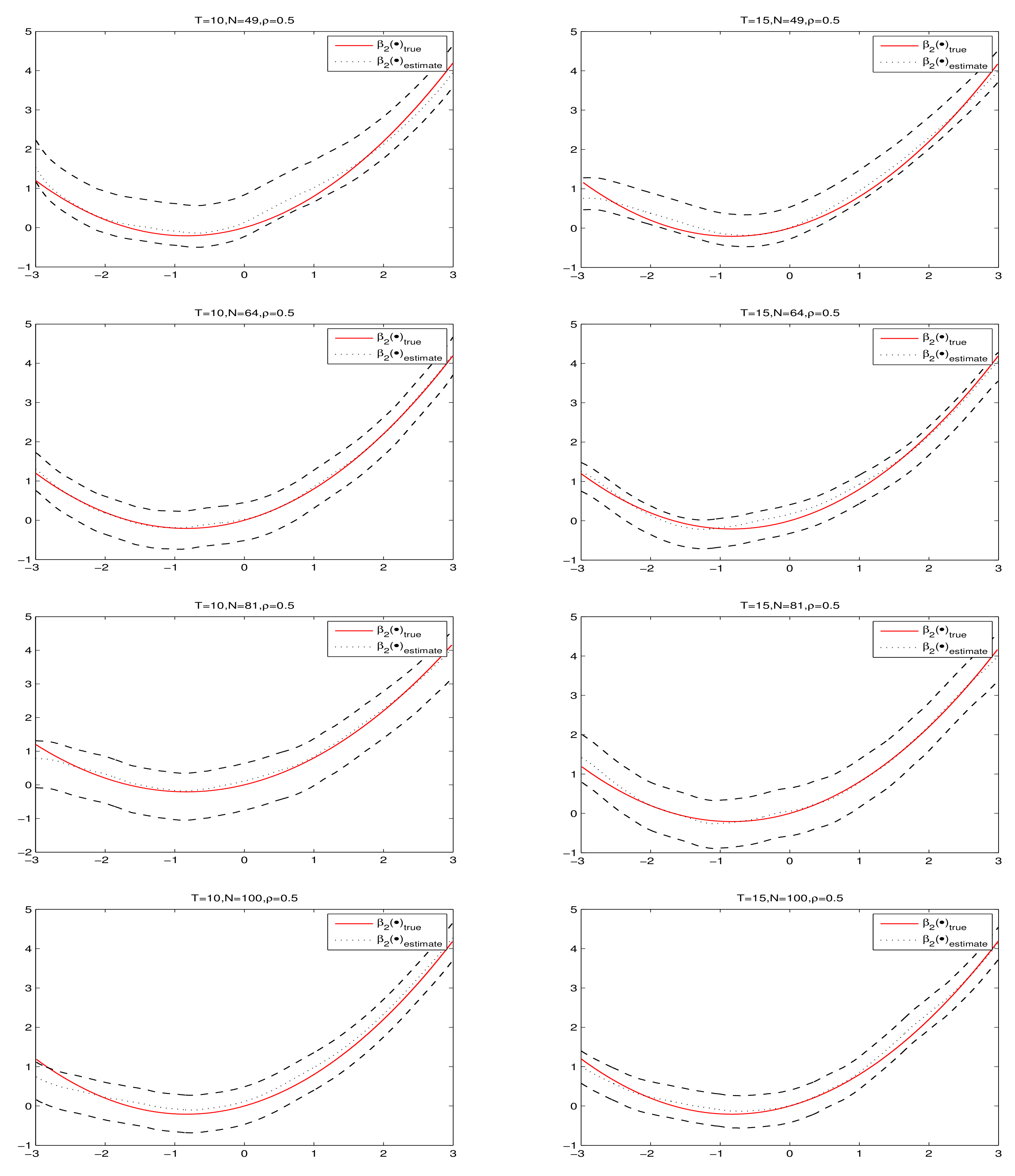
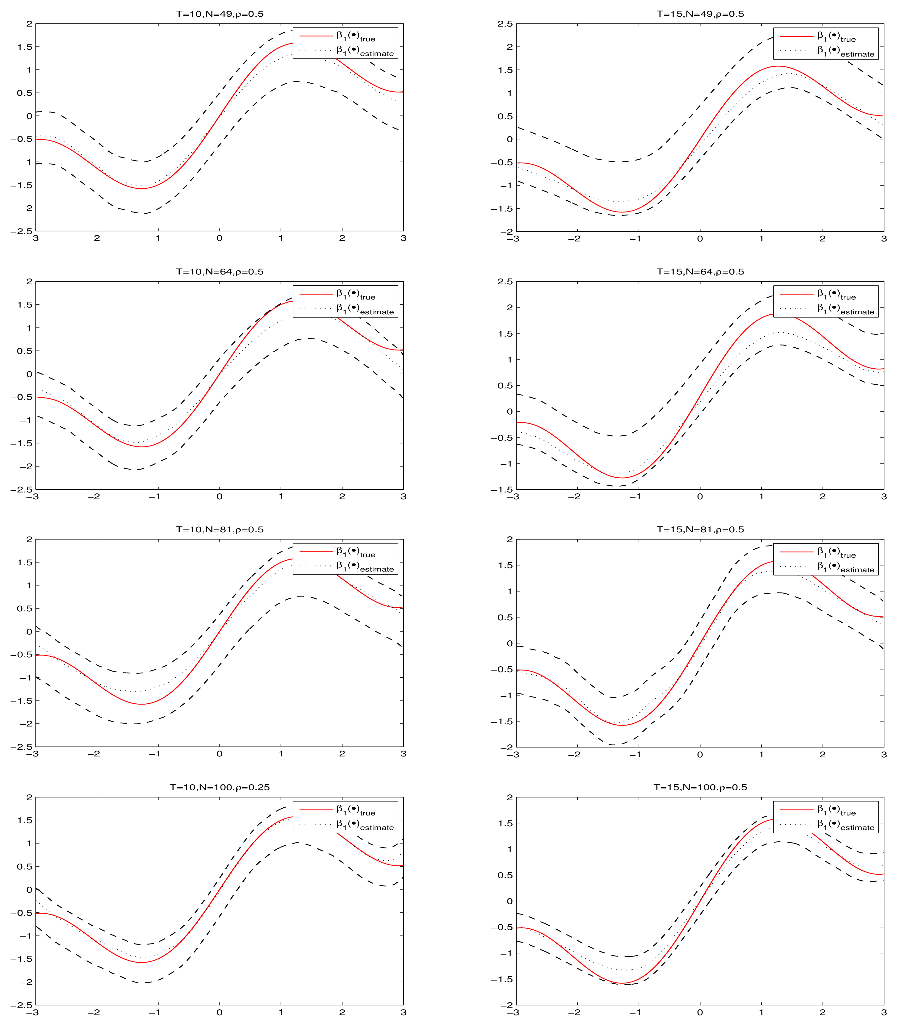
Figure 1 and Figure 2 present the fitting results and 95% confidence intervals of β 1 ( u ) and β 2 ( u ) under ρ = 0.5 , respectively, where the short dashed curves are the average fits over 500 simulations β ^ s ( u ) ( s = 1 , 2 ) by PQMLE, the solid curves are the true values of β s ( u ) ( s = 1 , 2 ) and the two long dashed curves are the corresponding 95% confidence bands. By observing every subgraph in Figure 1 and Figure 2, we can see that the short dashed curve is fairly close to solid curve and the corresponding confidence bandwidth is narrow. This illustrates that the nonparametric estimation procedure works well for small samples. To save space, we do not present the cases ρ = 0.25 and ρ = 0.75 because they had similar results as the case ρ = 0.5 .

5. Real Data Analysis

We applied the housing prices of Chinese city data to analyze the proposed model with real data. The data were obtained from the China Statistical Yearbook, the China City Statistical Yearbook and the China Statistical Yearbook for Regional Economies. Based on the panel data of related variables of 287 cities at/above the prefecture level (except the cities in Taiwan, Hong Kong and Macau) in China from 2011 to 2018, we explored the influencing factors of housing prices of Chinese cities by PLVCSARPM with random effects.
Taking [49,50,51] as references, we collected nine variables related to housing prices of China cities, including each city’s average selling price of residential houses (denoted by HP, yuan/sq.m), the expectation of housing price trends (EHP, %), population density (POD, person), annual per capita disposable income of urban households (ADI, yuan), loan–to–GDP ratio (MON, %), natural growth rate of population (NGR, %), sulphur dioxide emission (SDE, 10,000 tons), area of grassland (AOG, 10,000 hectares) and the value of buildings completed (VBC, yuan/sq.m). According to result of non-linear regression, the established model is given by
y i t = ρ ( W 0 Y t ) i + x i t β ( u i t ) + z i t α + b i + ε i t , 1 i 287 , 1 t 8 ,
where y i t represents the ith observation of ln(HP) at time t; z i t represents the ith observation of EHP at time t; x i t means the ith observation of POD, ln(ADI), MON, NGR, SDE and AOG at time t, respectively, u i t represents the ith observation of ln(VBC) at time t.
In order to transfer the asymmetric distribution of POD to nearly uniform distribution on (0,1), we set
P O D = P O D 1 / 3 min ( P O D 1 / 3 ) / max ( P O D 1 / 3 ) min ( P O D 1 / 3 ) .
The spatial weight matrix W 0 we adopted is calculated as follows:
w i j = e x p s i s j / k = 1 264 e x p s i s k ,
where s i = ( l o n g i t u d e i , l a t i t u d e i ) .
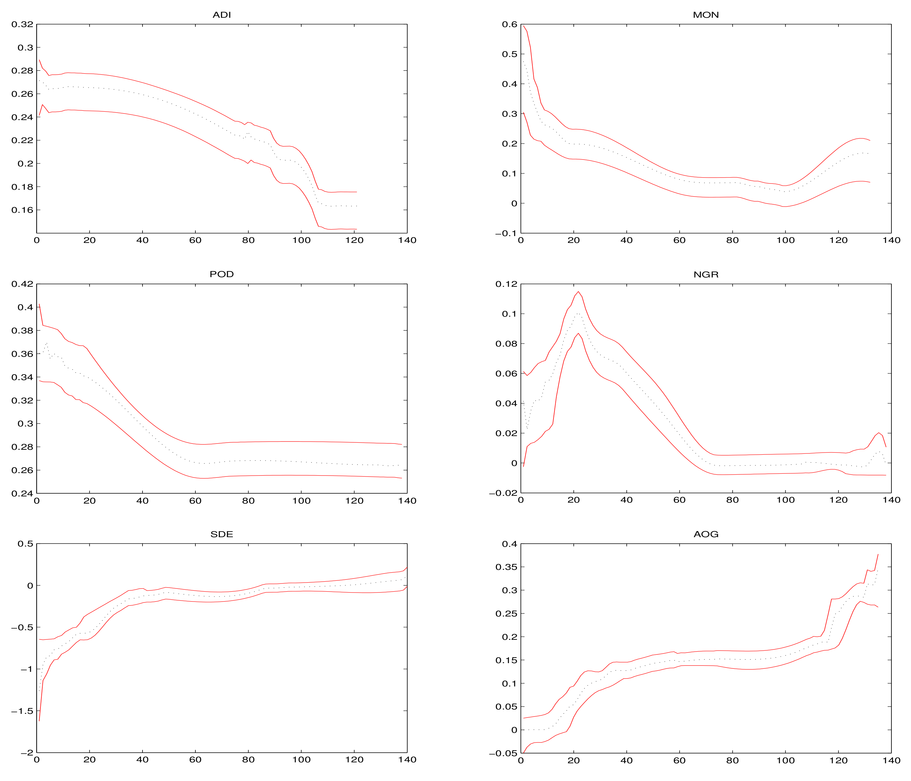
Figure 3 presents the estimation results and corresponding 95% confidence intervals of varying coefficient functions β s ( s = 1 , 2 , , 6 ) , where the black dashed line curves are the average fits over 500 simulations and the red solid lines are the corresponding 95% confidence bands. It can be seen from Figure 3 that all covariates variables have obvious non-linear effects on housing prices of Chinese cities.
The estimation results of parameters in the model (14) are reported in Table 7. It can be seen from Table 7: (1) all estimates of parameters are all significant; (2) spatial correlation coefficient ρ ^ = 0.3820 > 0 , which means there exists a spatial spill over effect for housing prices of Chinese cities; (3) α ^ = 0.9869 > 0 indicates that the expectation of housing price trends (EHP) has a promotional effect on housing prices of Chinese cities; (4) σ ^ ε 2 = 0.0163 shows that the growth of housing prices in different regions is relatively stable and is less affected by external fluctuations.

6. Conclusions

In this paper, we proposed PQMLE of PLVCSARPM with random effects. Our model has the following advantages: (1) It can overcome the “curse of dimensionality” in the nonparametric spatial regression model effectively. (2) It can simultaneously study the linear and non-linear effects of coveriates. (3) It can investigate the spatial correlation effect of response variables. Under some regular conditions, consistency and asymptotic normality of the estimators for parameters and varying coefficient functions were derived. Monte Carlo simulations showed the proposed estimators are well behaved with finite samples. Furthermore, the performance of the proposed method was also assessed on a set of asymmetric real data.
This paper only focused on the PQMLE of PLVCSARPM with random effects. In future research, we may try to extend our method to more general models, such as a partially linear varying coefficient spatial autoregressive model with autoregressive disturbances. In addition, we also need study the issues of Bayesian analysis, variable selection and quantile regression in these models.

Author Contributions

Supervision, S.L. and J.C.; software, S.L.; methodology, S.L.; writing—original draft preparation, S.L.; writing—review and editing, S.L., J.C. and D.C. All authors have read and agreed to the published version of manuscript.

Funding

This work was supported by the Natural Science Foundation of Fujian Province (2020J01170, 2021J01662); the Natural Science Foundation of China (12001105); the Program for Innovative Research Team in Science and Technology in Fujian Province University; and the Fujian Normal University Innovation Team Foundation “Probability and Statistics: Theory and Application” (IRTL1704).

Institutional Review Board Statement

Not applicable.

Informed Consent Statement

Not applicable.

Data Availability Statement

The data presented in this study are openly available in Reference [50].

Acknowledgments

The authors are deeply grateful to editors and anonymous referees for their careful reading and insightful comments. Their comments led us to significantly improve the paper.

Conflicts of Interest

The authors declare no conflict of interest.

Appendix A

To proceed with the proofs of main lemmas and theorems, we first provide two frequently used evident facts (see [14]).
Fact 1. If the row and column sums of the n × n matrices B 1 n and B 2 n are uniformly bounded in absolute value, then the row and column sums of B 1 n B 2 n are also uniformly bounded in absolute value.
Fact 2. If the row (resp. column) sums of B 1 n are uniformly bounded in absolute value and B 2 n is a conformable matrix whose elements are uniformly O ( o n ) , then so are the elements of B 1 n B 2 n (resp. B 2 n B 1 n ).
Proof of Lemma 2.
Recall S u = 1 N T D u W u D u . By straightforward calculation, it is not difficult to get
S u = S u 0 S u 1 S u 1 S u 2 ,
where S u l = 1 N T i = 1 N t = 1 T x i t x i t ( u i t u h ) l k h ( u i t u ) , l = 0 , 1 , 2 . Denote D i t l = x i t x i t k h ( u i t u ) ( u i t u h ) l , C t l = 1 N i = 1 N D i t l , then we have
S u l = 1 N T i = 1 N t = 1 T D i t l = 1 T t = 1 T C t l .
By Assumptions 1–3, we know
E C t l = 1 N i = 1 N E D i t l = 1 N i = 1 N E [ x i t x i t k h ( u i t u ) ( u i t u h ) l ] = E { E [ x i t x i t k h ( u i t u ) ( u i t u h ) l | u i t ] } = E { k h ( u i t u ) ( u i t u h ) l E ( x i t x i t | u i t ) } = E { k h ( u i t u ) ( u i t u h ) l Ω 11 ( u i t ) } = h 1 k ( ( u i t u ) / h ) f t ( u i t ) ( u i t u h ) l Ω 11 ( u i t ) d u i t = k ( υ ) f t ( u + h υ ) υ l Ω 11 ( u + h υ ) d υ = k ( υ ) [ f t ( u ) + h f t ( u ) υ + h 2 2 f t ( ξ ) υ 2 ] υ l Ω 11 ( u + h υ ) d υ = ( 1 + O ( h 2 ) ) f t ( u ) μ l Ω 11 ( u ) ,
where μ l = υ l k ( υ ) d υ and υ = u i t u h , D i t ( i = 1 , 2 , , N ) are i . i . d for any fixed t and l. According to Khinchine law of large numbers, we have C t l p E C t l . Therefore, it is not hard to get that
S u l = 1 T t = 1 T C t l = 1 T t = 1 T [ ( 1 + o p ( 1 ) ) E C t l ] = 1 T t = 1 T [ f t ( u ) μ l Ω 11 ( u ) + O ( h 2 ) ] ( 1 + o p ( 1 ) ) = 1 T t = 1 T [ f t ( u ) μ l Ω 11 ( u ) ] + O ( h 2 ) .
Let F ( u ) = l i m T 1 T t = 1 T f t ( u ) , then S u l p μ l F ( u ) Ω 11 ( u ) . Hence,
S u = S u 0 S u 1 S u 1 S u 2 p F ( u ) Ω 11 ( u ) 0 0 μ 2 Ω 11 ( u ) .
Proof of Lemma 3.
Recall T u = 1 N T D u W u Y ˜ . By straightforward calculation, we obtain
T u = 1 N T i = 1 N t = 1 T x i t y ˜ i t k h ( u i t u ) 1 N T i = 1 N t = 1 T x i t y ˜ i t ( u i t u h ) 1 k h ( u i t u ) = ^ T u , 0 T u , 1
where T u l = 1 N T i = 1 N t = 1 T x i t y ˜ i t ( u i t u h ) l k h ( u i t u ) for l = 0 , 1 . Then, it is not hard to obtain
T u l = 1 N T i = 1 N t = 1 T x i t y ˜ i t ( u i t u h ) l k h ( u i t u ) = 1 N T i = 1 N t = 1 T x i t x i t β 0 ( u i t ) ( u i t u h ) l k h ( u i t u ) + 1 N T i = 1 N t = 1 T x i t ( b i + ε i t ) ( u i t u h ) l k h ( u i t u ) .
For the first term of above equality in (A1), by similar proof procedures of Lemma 2, it is easily to get that
1 N T i = 1 N t = 1 T x i t x i t β 0 ( u i t ) ( u i t u h ) l k h ( u i t u ) p F ( u ) μ l Ω 11 ( u ) β 0 ( u ) .
For the second term of above equality in (A1), we obtain
E [ 1 N T i = 1 N t = 1 T x i t ( b i + ε i t ) ( u i t u h ) l k h ( u i t u ) ]
= E [ E [ 1 N T i = 1 N t = 1 T x i t ( b i + ε i t ) ( u i t u h ) l k h ( u i t u ) | u i t ] ] = E [ 1 N T i = 1 N t = 1 T E [ x i t ( b i + ε i t ) | u i t ] ( u i t u h ) l k h ( u i t u ) ] = 0 ,
and
V a r ( 1 N T i = 1 N t = 1 T x i t ( b i + ε i t ) ( u i t u h ) l k h ( u i t u ) ) = 1 ( N T ) 2 i = 1 N t = 1 T { E [ k h 2 ( u i t u ) ( u i t u h ) 2 l x i t x i t ] E [ ( b i + ε i t ) 2 ] } = o ( 1 ) .
Therefore,
T u = T u 0 T u 1 p F ( u ) μ l Ω 11 ( u ) β 0 ( u ) 0
Furthermore, by using (8) and Lemma 2, we easily know β ^ I N ( u ) p β 0 ( u ) . □
Proof of Lemma 5.
Its proof is analogous to Lemma 4.2 in [34] and Theorem 3.2 in [12]. The major difference is that our model is panel model with random effects instead of sectional model.
In order to prove Σ θ 0 is positive definite, we need only prove that κ = 0 according to Σ θ 0 κ = 0 , where κ = ( κ 1 , κ 2 , κ 3 , κ 4 ) , κ 1 , κ 2 , κ 3 are constants, and κ 4 is a q dimension column vector.
It follows from Σ θ 0 κ = 0 that:
κ 2 = 2 ( σ ε 0 2 + T σ b 0 2 ) t r ( G 0 H ) [ T ( σ ε 0 2 + T σ b 0 2 ) σ ε 4 + T ( σ ε 0 2 + T σ b 0 2 ) σ ε 0 4 ] N T ( σ ε 0 2 + T σ b 0 2 ) 2 + N σ ε 0 4 κ 1 ,
κ 3 = t r ( G 0 H ) ( σ ε 0 2 + T σ b 0 2 ) [ 2 N T ( σ ε 0 2 + T σ b 0 2 ) + 2 N σ ε 0 4 T 2 σ ε 0 4 ( σ ε 0 2 + T σ b 0 2 ) + T 2 ( σ ε 0 2 + T σ b 0 2 ) T σ ε 0 4 ] N T 2 ( σ ε 0 2 + T σ b 0 2 ) + N T σ ε 0 4 κ 1
and
κ 4 = T σ b 0 2 ϕ Z Z 1 ϕ Q 0 Z κ 1 .
By straightforward calculations, it can be simplified to prove
( T σ b 0 2 ϕ Q 0 Z ϕ Z Z 1 ϕ Q 0 Z + ϕ Q 0 Q 0 ) κ 1 + c 3 κ 1 + [ ( σ ε 0 2 + T σ b 0 2 ) 2 t r ( G 0 G 0 ) ( σ ε 0 2 + T σ b 2 ) σ ε 0 2 t r ( G 0 2 ) ] κ 1 = 0 ,
where c 3 = T σ ε 0 4 ( σ ε 0 2 + σ b 0 2 ) + T ( σ ε 0 2 + σ b 0 2 ) σ ε 0 4 > 0 .
By Lemma 4 in [43], it is easy to obtain that ( σ ε 0 2 + T σ b 0 2 ) 2 t r ( G 0 G 0 ) ( σ ε 0 2 + T σ b 0 2 ) σ ε 2 t r ( G 0 2 ) > 0 . Furthermore, according to Assumption 6, T σ b 0 2 ϕ Q 0 Z ϕ Z Z 1 ϕ Q 0 Z + ϕ Q 0 Q 0 0 . Thus, we have κ 1 = 0 and so κ = 0 . This completes the proof. □
Proof of Theorem 1.
Let { α ^ , ρ ^ } = arg max α , ρ l n L ˜ ( α , ρ ) and { α 0 , ρ 0 } = arg max α , ρ l n L ( α , ρ ) . We adopt the idea of Theorem 3.2 in [12] to prove the consistency of ρ ^ and α ^ . By the Consistency of Extrema Estimators in [52], it suffices to show that
1 N T [ l n L ˜ ( α , ρ ) l n L ( α , ρ ) ] = o p ( 1 ) ,
where
l n L ˜ ( α , ρ ) = N ( T 1 ) 2 l n σ ^ ε I N 2 N 2 l n ( σ ^ ε I N 2 + T σ ^ b I N 2 ) + l n | A ( ρ ) | ,
and
l n L ( α , ρ ) = N ( T 1 ) 2 l n σ ˜ ε 2 N 2 l n ( σ ˜ ε 2 + T σ ˜ b 2 ) + l n | A ( ρ ) | .
By straightforward calculation, we have
1 N T [ l n L ˜ ( α , ρ ) l n L ( α , ρ ) ] = T 1 2 T ( l n σ ˜ ε 2 l n σ ^ ε I N 2 ) + 1 2 T [ l n ( σ ˜ ε 2 + T σ ˜ b 2 ) l n ( σ ^ ε I N 2 + T σ ^ b I N 2 ) ] .
Therefore, it only needs to prove that
σ ^ ε I N 2 σ ˜ ε 2 = o p ( 1 )
and
σ ^ b I N 2 σ ˜ b 2 = o p ( 1 ) .
We first prove (A2) holds.
it is obvious that
σ ^ ε I N 2 = 1 N ( T 1 ) [ Y ˜ X β ^ I N ( u ) ] ( I H ) [ Y ˜ X β ^ I N ( u ) ] = 1 N ( T 1 ) [ Y ˜ X β ( u ) ] ( I H ) [ Y ˜ X β ( u ) ] + 2 N ( T 1 ) [ Y ˜ X β ( u ) ] ( I H ) ( X β ( u ) X β ^ I N ( u ) ) + 1 N ( T 1 ) ( X β ( u ) X β ^ I N ( u ) ) ( I H ) ( X β ( u ) X β ^ I N ( u ) ) = σ ˜ ε 2 + 2 N ( T 1 ) [ Y ˜ X β ( u ) ] ( I H ) ( X β ( u ) X β ^ I N ( u ) ) + 1 N ( T 1 ) ( X β ( u ) X β ^ I N ( u ) ) ( I H ) ( X β ( u ) X β ^ I N ( u ) ) .
Thus, it is necessary to prove the last two terms of above equality converge to 0 in probability. By Lemma 3 and Assumption 1(iv), we have X β ( u ) X β ^ I N ( u ) = o p ( 1 ) . Moreover,
[ Y ˜ X β ( u ) ] ( I H ) = ( U b + ε ) ( I H ) = ( ε 11 T 1 t = 1 T ε 1 t , ε 12 T 1 t = 1 T ε 1 t , , ε N T T 1 t = 1 T ε N t ) .
By weak law of large numbers,
1 N T i = 1 N t = 1 T | ε i t T 1 t = 1 T ε i t | 2 N T i = 1 N t = 1 T | ε i t | 2 ( 1 N T i = 1 N t = 1 T ε i t 2 ) 1 2 p 2 σ ε .
Thus
2 N ( T 1 ) [ Y ˜ X β ( u ) ] ( I H ) [ X β ( u ) X β ^ I N ( u ) ] = o p ( 1 )
It follows from X β ( u ) X β ^ I N ( u ) = o p ( 1 ) that
1 N ( T 1 ) [ X β ( u ) X β ^ I N ( u ) ] ( I H ) [ X β ( u ) X β ^ I N ( u ) ] 1 N ( T 1 ) [ X β ( u ) X β ^ I N ( u ) ] [ X β ( u ) X β ^ I N ( u ) ] = o p ( 1 )
By (A4) and (A5), we have
σ ^ ε I N 2 σ ˜ ε 2 = o p ( 1 ) .
Similar to the proof of (A2), it is not difficult to verify that σ ^ b I N 2 σ ˜ b 2 = o p ( 1 ) . According to the continuity of l n ( · ) , we have
1 N T [ l n L ˜ ( α , ρ ) l n L ( α , ρ ) ] = o p ( 1 ) .
Consequently, the consistency of ρ ^ and α ^ are proved. □
Proof of Theorem 2.
It follows by straightforward calculation that
T u = 1 N T D u W u Y ˜ = 1 N T i = 1 N t = 1 T x i t y ˜ i t k h ( u i t u ) 1 N T i = 1 N t = 1 T x i t y ˜ i t ( u i t u h ) 1 k h ( u i t u ) = ^ T u , 0 T u , 1 ,
where T u , l = 1 N T i = 1 N t = 1 T x i t y ˜ i t ( u i t u h ) l k h ( u i t u ) , l = 0 , 1 .
Moreover, β ^ ( u ) = e 0 [ D u W u D u ] 1 D u W u Y ˜ ^ = e 0 S u 1 T ^ u , where T ^ u = D u W u Y ˜ ^ = T ^ u , 0 T ^ u , 1 and T ^ u , l = 1 N T i = 1 N t = 1 T x i t y ˜ ^ i t ( u i t u h ) l k h ( u i t u ) , l = 0 , 1 . By Theorem 1, it is easy to obtain that
y ˜ ^ i t = y i t ρ ^ ( W 0 Y t ) i z i t α ^ = y i t ( ρ + ρ ^ ρ ) ( W 0 Y t ) i z i t ( α + α ^ α ) = y ˜ ( 1 + o p ( 1 ) ) .
Thus,
T ^ u , l = 1 N T i = 1 N t = 1 T x i t y ˜ ^ i t ( u i t u h ) l k h ( u i t u ) = ( 1 + o p ( 1 ) ) 1 N T i = 1 N t = 1 T x i t y ˜ i t ( u i t u h ) l k h ( u i t u ) = ( 1 + o p ( 1 ) ) T u , l .
Therefore, β ^ ( u ) = e 0 S u 1 T ^ u = ( 1 + o p ( 1 ) ) e 0 S u 1 T u = ( 1 + o p ( 1 ) ) β ^ I N ( u ) . Furthermore, we have β ^ ( u ) β 0 ( u ) = β ^ ( u ) β ^ I N ( u ) + β ^ I N ( u ) β 0 ( u ) = o p ( 1 ) by using Lemma 3. □
Proof of Theorem 3.
By Theorem 1, we have
σ ˜ ε 2 σ ^ ε I N 2 = o p ( 1 ) , σ ˜ b 2 σ ^ b I N 2 = o p ( 1 ) .
To prove our conclusions, we only need to verify that
σ ˜ ε 2 σ ε 0 2 = o p ( 1 ) , σ ˜ b 2 σ b 0 2 = o p ( 1 )
and
σ ^ ε 2 σ ^ ε I N 2 = o p ( 1 ) , σ ^ b 2 σ ^ b I N 2 = o p ( 1 ) .
Firstly, we prove (A6) holds. It is easy to know
σ ˜ ε 2 = 1 N ( T 1 ) [ A ( ρ ) Y X β ( u ) Z α ] ( I H ) [ A ( ρ ) Y X β ( u ) Z α ] = 1 N ( T 1 ) ( U b + ε ) ( I H ) ( U b + ε ) = 1 N ( T 1 ) [ i = 1 N t = 1 T ε i t 2 1 T i = 1 N ( t = 1 T ε i t 2 ) 2 ] = 1 N ( T 1 ) t = 1 T i = 1 N ε i t 2 1 ( T 1 ) [ 1 N T i = 1 N ( t = 1 T ε i t ) 2 ] .
According to Khinchine law of large numbers, we have
1 N ( T 1 ) i = 1 N t = 1 T ε i t 2 P E ( ε i t 2 ) = σ ε 0 2
and
1 N T i = 1 N ( t = 1 T ε i t ) 2 = 1 N T i = 1 N t = 1 T ε i t 2 + 2 N T i = 1 N j k T ε i j ε i k P E ( ε i t 2 ) = σ ε 0 2 .
Thus, 1 ( T 1 ) [ 1 N T i = 1 N ( t = 1 T ε i t ) 2 ] = o p ( 1 ) . Therefore, σ ˜ ε 2 σ ε 0 2 = o p ( 1 ) . By similar way, it is not hard to get σ ˜ b 2 σ ^ b 0 2 = o p ( 1 ) .
Secondly, we prove (A7). By (13), Theorem 1 and Theorem 2, a simple calculation yields
σ ^ ε 2 = 1 N ( T 1 ) [ A ( ρ ^ ) Y X β ^ ( u ) Z α ^ ] ( I H ) [ A ( ρ ^ ) Y X β ^ ( u ) Z α ^ ] = 1 N ( T 1 ) ( Y ˜ ^ X β ^ ( u ) ) ( I H ) ( Y ˜ ^ X β ^ ( u ) ) = 1 N ( T 1 ) ( 1 + o p ( 1 ) ) ( Y ˜ X β ^ I N ( u ) ) ( I H ) ( 1 + o p ( 1 ) ) ( Y ˜ X β ^ I N ( u ) ) = ( 1 + o p ( 1 ) ) σ ^ ε I N 2 .
Thus, σ ^ ε 2 σ ^ ε I N 2 = o p ( 1 ) . By a similar way, we can obtain σ ^ b 2 σ ^ b I N 2 = o p ( 1 ) . This completes the proof. □
Proof of Theorem 4.
By Taylor expansion of l n L ˜ ( θ ) θ | θ = θ ^ = 0 at θ 0 , we have
l n L ˜ ( θ ) θ | θ = θ 0 + 2 l n L ˜ ( θ ) θ θ | θ = θ ˜ ( θ ^ θ 0 ) = 0 ,
where θ ˜ = ( ρ ˜ , α ˜ , σ ˜ b 2 , σ ˜ ε 2 ) and θ ˜ lies between θ ^ and θ 0 . By Theorem 1 and Theorem 3, we easily know that θ ˜ converges to θ 0 in probability.
Denote
l n L ˜ ( θ 0 ) θ = ^ l n L ˜ ( θ ) θ | θ = θ 0 , 2 l n L ˜ ( θ 0 ) θ θ = ^ 2 l n L ˜ ( θ ) θ θ | θ = θ 0 , 2 l n L ˜ ( θ ˜ ) θ θ = ^ 2 l n L ˜ ( θ ) θ θ | θ = θ ˜ .
Thus,
N T ( θ ^ θ 0 ) = ( 1 N T 2 l n L ˜ ( θ ˜ ) θ θ ) 1 1 N T l n L ˜ ( θ 0 ) θ .
Next, we prove
1 N T 2 l n L ˜ ( θ ˜ ) θ θ 1 N T 2 l n L ( θ 0 ) θ θ = o p ( 1 )
and
1 N T l n L ˜ ( θ 0 ) θ D N ( 0 , Σ θ 0 + Ω θ ) .
To prove (A8), we need to show that each element of 1 N T 2 l n L ˜ ( θ ˜ ) θ θ 1 N T 2 l n L ( θ 0 ) θ θ converges to 0 in probability. It is not difficult to get
1 N T 2 l n L ( θ 0 ) ρ ρ = 1 N T [ 1 σ ε 0 2 + T σ b 0 2 ( W Y ) ( I S ) H ( I S ) W Y + 1 σ ε 0 2 ( W Y ) ( I S ) ( I H ) ( I S ) W Y + t r ( G 0 2 ) ] ,
1 N T 2 l n L ( θ 0 ) ρ σ ε 2 = 1 N T Y W ( I S ) [ H ( σ ε 0 2 + T σ b 0 2 ) 2 + I H σ ε 0 4 ] ( I S ) [ A ( ρ 0 ) Y Z α 0 ] ,
1 N T 2 l n L ( θ 0 ) ρ σ b 2 = 1 N T Y W ( I S ) H σ ε 0 2 + T σ b 0 2 ( I S ) [ A ( ρ 0 ) Y Z α 0 ] ,
1 N T 2 l n L ( θ 0 ) ρ α = 1 N T Y W ( I S ) ( H σ ε 0 2 + T σ b 0 2 + I H σ ε 0 2 ) ( I S ) Z ,
1 N T 2 l n L ( θ 0 ) σ ε 2 σ ε 2 = 1 N T [ A ( ρ 0 ) Y Z α ] ( I S ) [ H ( σ ε 0 2 + T σ b 0 2 ) 3 + I H σ ε 0 6 ] ( I S ) [ A ( ρ 0 ) Y Z α 0 ] + T 1 T σ ε 0 4 + 1 2 T ( σ ε 0 2 + T σ b 0 2 ) 2 ,
1 N T 2 l n L ( θ 0 ) σ ε 2 σ b 2 = 1 2 ( σ ε 0 2 + T σ b 0 2 ) 2 1 2 N ( σ ε 0 2 + T σ b 0 2 ) 3 [ A ( ρ 0 ) Y Z α 0 ] ( I S ) H ( I S ) [ A ( ρ 0 ) Y Z α 0 ] ,
1 N T 2 l n L ( θ 0 ) σ ε 2 α = 1 N T Z ( I S ) [ H ( σ ε 0 2 + T σ b 0 2 ) 2 + I H σ ε 0 4 ] ( I S ) [ A ( ρ 0 ) Y Z α 0 ] ,
1 N T 2 l n L ( θ 0 ) σ b 2 σ b 2 = T 2 ( σ ε 0 2 + T σ b 0 2 ) 2 T N ( σ ε 0 2 + T σ b 0 2 ) 3 [ A ( ρ 0 ) Y Z α 0 ] ( I S ) H ( I S ) [ A ( ρ 0 ) Y Z α 0 ] ,
1 N T 2 l n L ( θ 0 ) σ b 2 α = 1 N ( σ ε 0 2 + T σ b 0 2 ) 2 Z ( I S ) H ( I S ) [ A ( ρ 0 ) Y Z α 0 ] ,
1 N T 2 l n L ( θ 0 ) α α = 1 N T ( σ ε 0 2 + T σ b 0 2 ) Z ( I S ) ( I S ) Z .
By mean value theorem, Assumption 2 ( i v ) and Lemma 5, we have
1 N T ( 2 l n L ( θ ˜ ) ρ 2 2 l n L ( θ 0 ) ρ 2 ) = 1 N T ( 1 σ ˜ ε 2 + T σ ˜ b 2 1 σ ε 0 2 + T σ b 0 2 ) ( W Y ) ( I S ) H ( I S ) W Y + 1 N T ( 1 σ ˜ ε 2 1 σ ˜ ε 0 2 ) ( W Y ) ( I S ) ( I H ) ( I S ) W Y + 1 N T [ t r ( G 2 ( ρ ˜ ) ) t r ( G 2 ( ρ 0 ) ) ] = 2 N T t r ( G 3 ( ρ ˜ * ) ) ( ρ ˜ ρ 0 ) + o p ( 1 ) = o p ( 1 ) ,
where ρ ˜ * lies between ρ ˜ and ρ 0 . Similarly, we have
1 N T 2 l n L ˜ ( θ ˜ ) θ θ 1 N T 2 l n L ( θ 0 ) θ θ = o p ( 1 ) .
To prove (A9), we adopt the idea of [12]. It is easy to obtain that the components of 1 N T l n L ˜ ( θ 0 ) θ are linear or quadratic functions of U b + ε and their means are all o p ( 1 ) . Under Assumption 1, we have that 1 N T l n L ˜ ( θ 0 ) θ is asymptotically normal distributed with 0 means by using the CLT for linear-quadratic forms of Theorem 1 in [53]. In the following, we calculate its variance. According to the structure of the Fisher information matrix, we know that
V a r ( 1 N T l n L ˜ ( θ 0 ) θ ) = E ( 1 N T l n L ˜ ( θ 0 ) θ · 1 N T l n L ˜ ( θ 0 ) θ ) = E ( 1 N T 2 l n L ( θ 0 ) θ θ ) + E ( Ω θ N T ) ,
where
1 N T 2 l n L ( θ 0 ) θ θ = { σ b 2 E [ Q 0 P Q 0 ] N ( σ ε 0 2 + T σ b 0 2 ) σ ε 0 2 + σ b 0 2 [ t r ( G 0 G 0 ) + t r ( G 0 H G 0 ) ] N σ ε 0 2 + t r ( G 0 G 0 ) t r ( G 0 2 ) N T } * * * t r ( G 0 H ) N T ( σ ε 0 2 + T σ b 0 2 ) [ t r ( G 0 ) t r ( G 0 H ) ] N T σ ε 0 4 1 2 σ ε 0 4 * * t r ( G 0 H ) N T ( σ ε 0 2 + T σ b 0 2 ) 1 2 ( σ ε 0 2 + T σ b 0 2 ) 2 T 2 ( σ ε 0 2 + T σ b 0 2 ) 2 * σ b 2 E [ Q 0 P Z ] N ( σ ε 0 2 + T σ b 0 2 ) σ ε 0 2 0 0 E [ Z P Z ] N T ( σ ε 0 2 + T σ b 0 2 ) + o p ( 1 ) ,
Ω θ N T = Ω θ N T 11 Ω θ N T 12 Ω θ N T 13 Ω θ N T 14 * Ω θ N T 22 Ω θ N T 23 Ω θ N T 24 * * Ω θ N T 33 Ω θ N T 34 * * * Ω θ N T 44 .
Let μ b 03 and μ ε 03 be the third moments of b and ε , respectively; μ b 04 and μ ε 04 be the forth moments of b and ε , respectively; and A i i be the ii-th element of A. By using the Lemma 5 and the facts that E ( U n A n U n ) = σ 0 2 t r ( A n ) , E ( U n A n U n U n B n U n ) = ( μ 4 3 σ 0 4 ) i = 1 n a n , i i b n , i i + σ 0 4 [ t r ( A n B n ) + t r ( A n B n ) + t r ( A n B n ) ] , it follows by straightforward calculation that
Ω θ N T 11 = ( μ b 04 3 σ b 0 4 ) i = 1 N T ( U H U ) i i [ U U U H U ] i i + ( μ ε 04 3 σ ε 0 4 ) i = 1 N T H i i ( I H ) i i N T + μ b 3 Q 0 H U d i a g ( U G 0 U U H G 0 U ) + μ ε 03 Q 0 H d i a g ( G 0 H G 0 ) N T 2 σ ε 0 2 + ( μ b 04 3 σ b 0 4 ) i = 1 N T ( U H U ) i i 2 + ( μ ε 04 3 σ ε 0 4 ) i = 1 N T ( I H ) i i N T 2 + μ b 03 Q 0 H U d i a g ( U H G 0 U ) + μ ε 03 Q 0 H d i a g ( H G 0 ) N T 2 ( σ ε 0 2 + T σ b 2 ) ,
Ω θ N T 12 = ( μ b 04 3 σ b 0 4 ) i = 1 N T [ ( U G 0 U U G 0 H U ) i i [ U U U H U ] i i ] 2 N T σ ε 0 6 + + ( μ ε 04 3 σ ε 0 4 ) i = 1 N T [ ( G 0 G 0 H ) i i ( I H ) i i ] 2 N T σ ε 0 6 + ( μ b 04 3 σ b 0 4 ) i = 1 N T [ ( U G 0 H U ) i i ( U U U H U ) i i ] + ( μ ε 04 3 σ ε 0 4 ) i = 1 N T [ ( G 0 H ) i i ( I H ) i i ] 2 N T σ ε 0 4 ( σ ε 0 2 + T σ b 0 2 )
+ ( μ b 04 3 σ b 0 4 ) i = 1 N T [ ( U G 0 H U ) i i ( U U U H U ) i i ] + ( μ ε 04 3 σ ε 0 4 ) i = 1 N T [ ( G 0 H ) i i ( I H ) i i ] 2 N T σ ε 0 2 ( σ ε 0 2 + T σ b 0 2 ) 2 + ( μ b 04 3 σ b 0 4 ) i = 1 N T ( U G 0 H U ) i i + ( μ ε 04 3 σ ε 0 4 ) i = 1 N T [ ( G 0 H ) i i H i i ] 2 N T ( σ ε 0 2 + T σ b 0 2 ) 3 + μ b 03 Q 0 H U d i a g [ U U U H U ] + μ ε 03 Q 0 H d i a g ( I H ) 2 N T σ ε 0 4 ( σ ε 0 2 + T σ b 0 2 ) + μ b 03 Q 0 ( I H ) U d i a g ( U H U ) + μ ε 03 Q 0 ( I H ) d i a g ( H ) 2 N T σ ε 0 2 ( σ ε 0 2 + T σ b 0 2 ) 2 + μ b 03 Q 0 H U d i a g ( U H U ) + μ ε 03 Q 0 H d i a g ( H ) 2 N T ( σ ε 0 2 + T σ b 0 2 ) 3 ,
Ω θ N T 13 = μ b 03 Q 0 H U d i a g ( U H U ) + μ ε 03 Q 0 H d i a g ( H ) 2 N ( σ ε 0 2 + T σ b 0 2 ) 3 + μ b 03 Q 0 ( I H ) U d i a g ( U H U ) + μ ε 03 Q 0 ( I H ) d i a g ( H ) 2 N σ ε 0 2 ( σ ε 0 2 + T σ b 0 2 ) 2 + ( μ b 04 3 σ b 0 4 ) i = 1 N T [ ( U G 0 H U ) i i ( U U U H U ) i i ] + ( μ ε 04 3 σ ε 0 4 ) i = 1 N T [ ( G 0 H ) i i ( I H ) i i ] 2 N σ ε 0 2 ( σ ε 0 2 + T σ b 0 2 ) 2 + ( μ b 04 3 σ b 0 4 ) i = 1 N T [ ( U G 0 H U ) i i ( U H U ) i i ] + ( μ ε 04 3 σ ε 0 4 ) i = 1 N T [ ( G 0 H ) i i H i i ] 2 N ( σ ε 0 2 + T σ b 0 2 ) 3 ,
Ω θ N T 14 = 0 ,
Ω θ N T 22 = ( μ b 04 3 σ b 0 4 ) i = 1 N T [ ( U H U ) i i ( U U U H U ) i i ] + ( μ ε 04 3 σ ε 0 4 ) i = 1 N T [ H i i ( I H ) i i ] σ ε 0 4 ( σ ε 0 2 + T σ b 0 2 ) 2 + ( μ b 04 3 σ b 0 4 ) i = 1 N T ( U U U H U ) i i 2 + ( μ ε 04 3 σ ε 0 4 ) i = 1 N T ( I H ) i i 2 σ ε 0 8 + ( μ b 04 3 σ b 0 4 ) i = 1 N T ( U H U ) i i 2 + ( μ ε 04 3 σ ε 0 4 ) i = 1 N T H i i 2 N T ( σ ε 0 2 + T σ b 0 2 ) 4 ,
Ω θ N T 23 = ( μ b 04 3 σ b 0 4 ) i = 1 N T [ ( U H U ) i i ( U U U H U ) i i ] + ( μ ε 04 3 σ ε 0 4 ) i = 1 N T [ H i i ( I H ) i i ] 4 N σ ε 0 4 ( σ ε 0 2 + T σ b 0 2 ) 2 + ( μ b 04 3 σ b 0 4 ) i = 1 N T ( U H U ) i i 2 + ( μ ε 04 3 σ ε 0 4 ) i = 1 N T H i i 2 4 N ( σ ε 0 2 + T σ b 0 2 ) 3 ,
Ω θ N T 24 = μ b 03 Z H U d i a g ( U H U ) + μ ε 03 Z H d i a g ( H ) 2 N T ( σ ε 0 2 + T σ b 0 2 ) 3 + μ b 03 Z ( I H ) U d i a g ( U H U ) + μ ε 03 Z ( I H ) d i a g ( H ) 2 N T σ ε 0 2 ( σ ε 0 2 + T σ b 0 2 ) 2 + μ b 03 Z ( I H ) U d i a g ( U U U H U ) + μ ε 03 Z ( I H ) d i a g ( I H ) 2 N T 2 σ ε 0 6 + μ b 03 Z H U d i a g ( U U U H U ) + μ ε 03 Z H d i a g ( I H ) 2 N T σ ε 0 4 ( σ ε 0 2 + T σ b 0 2 ) ,
Ω θ N T 33 = T [ ( μ b 04 3 σ b 0 4 ) i = 1 N T ( U H U ) i i 2 + ( μ ε 04 3 σ ε 0 4 ) i = 1 N T H i i 2 ] 4 N ( σ ε 0 2 + T σ b 0 2 ) 4
Ω θ N T 34 = μ b 03 Z ( I H ) U d i a g ( U H U ) + μ ε 03 Z ( I H ) d i a g ( H ) 2 N T σ ε 0 2 ( σ ε 0 2 + T σ b 0 2 ) + μ b 03 Z H U d i a g ( U H U ) + μ ε 03 Z H d i a g ( H ) 2 N ( σ ε 0 2 + T σ b 0 2 ) 2 ,
Ω θ N T 44 = 0 .
Particularly, it is not difficult to know that Ω θ = O ( 1 T ) = o ( 1 ) when b i and ε i t are normally distributed, respectively. This completes the proof. □
Proof of Theorem 5.
According to Lemma 2, we know
S u = Λ ( u ) + o p ( 1 ) ,
where Λ ( u ) = F u d i a g ( Ω 11 ( u ) , μ 2 Ω 11 ( u ) ) . By using the fact that ( A + B ) 1 = A 1 A 1 ( I + B A 1 ) 1 B A 1 , we have
δ ^ = β ^ I N ( u ) h β ^ ˙ I N ( u ) = S u 1 T u P Λ 1 ( u ) T u .
Denote R u = 1 N T D u W u ( U b + ε ) . By using Lemma 1 and Taylor expansion of β 0 ( u i t ) at u, it is not difficult to get
T u R u = S u β 0 ( u ) h β ˙ 0 ( u ) + 1 2 h 2 1 N T i = 1 N t = 1 T k h ( u i t u ) x i t x i t ( u i t u h ) 2 β ¨ 0 ( u ) 1 N T i = 1 N t = 1 T k h ( u i t u ) x i t x i t ( u i t u h ) 3 β ¨ 0 ( u ) + o ( h 2 ) .
According to the proof procedure of Lemma 2, we know
E [ k h ( u i t u ) x i t x i t ( u i t u h ) 2 β ¨ 0 ( u ) ] = μ 2 f ( u ) Ω 11 ( u ) β ¨ 0 ( u ) .
Thus
β ^ I N ( u ) β 0 ( u ) = e 0 Λ 1 ( u ) R u + e 0 1 2 h 2 Λ 1 ( u ) 1 N T i = 1 N t = 1 T k h ( u i t u ) x i t x i t ( u i t u h ) 2 β ¨ 0 ( u ) 1 N T i = 1 N t = 1 T k h ( u i t u ) x i t x i t ( u i t u h ) 3 β ¨ 0 ( u ) + o ( h 2 ) = 1 N T i = 1 N t = 1 T k h ( u i t u ) x i t ( b i + ε i t ) [ F ( u ) Ω ( u ) ] 1 + 1 2 h 2 μ 2 β ¨ 0 ( u ) + o ( h 2 ) .
Define ς i t = N T h i = 1 N t = 1 T k h ( u i t u ) x i t ( b i + ε i t ) , then
E ( ς i t ) = 0
and
E ( ς i t 2 ) = h E [ k h 2 ( u i t u ) x i t x i t ( b i + ε i t ) 2 ] = υ 0 ( σ ε , 0 2 + σ b , 0 2 ) F ( u ) Ω 11 ( u ) + o p ( 1 ) .
According to CLT, we have
N T h 1 N T i = 1 N t = 1 T k h ( u i t u ) x i t ( b i + ε i t ) D N ( 0 , υ 0 ( σ ε , 0 2 + σ b , 0 2 ) F ( u ) Ω 11 ( u ) )
and
N T h ( β ^ I N ( u ) β 0 ( u ) φ ( u ) ) D N ( 0 , γ 2 ( u ) ) ,
where φ ( u ) = 1 2 h 2 μ 2 β ¨ 0 ( u ) and γ 2 ( u ) = υ 0 ( σ ε , 0 2 + σ b , 0 2 ) [ F ( u ) Ω 11 ( u ) ] 1 . Furthermore, if N T h 5 0 , then
N T h ( β ^ I N ( u ) β 0 ( u ) ) D N ( 0 , γ 2 ( u ) ) .
By Lemma 3 and Theorem 2, we obtain that
N T h ( β ^ ( u ) β 0 ( u ) φ ( u ) ) D N ( 0 , γ 2 ( u ) ) .
In particular, when N T h 5 0 , N T h ( β ^ ( u ) β 0 ( u ) ) D N ( 0 , γ 2 ( u ) ) holds. □

References

  1. Elhorst, J.P. Spatial Econometrics: From Cross-sectional Data to Spatial Panels; Springer: Berlin, Germany, 2014. [Google Scholar]
  2. Brueckner, J.K. Strategic interaction among local governments: An overview of empirical studies. Int. Reg. Sci. Rev. 2003, 26, 175–188. [Google Scholar] [CrossRef] [Green Version]
  3. LeSage, J.P.; Pace, R.K. Introduction to Spatial Econometrics; CRC Press, Taylor & Francis Group: Boca Raton, MA, USA, 2009. [Google Scholar]
  4. Elhorst, J.P. Applied spatial econometrics: Raising the bar. Spat. Econ. Anal. 2010, 5, 9–28. [Google Scholar] [CrossRef]
  5. Allers, M.A.; Elhorst, J.P. Tax mimicking and yardstick competition among governments in the Netherlands. Int. Tax Public Financ. 2005, 12, 493–513. [Google Scholar]
  6. Cliff, A.D.; Ord, J.K. Spatial Autocorrelation; Pion Ltd.: London, UK, 1973. [Google Scholar]
  7. Anselin, L. Spatial Econometrics: Methods and Models; Kluwer Academic: Dordrecht, The Netherlands, 1988. [Google Scholar]
  8. Anselin, L.; Bera, A.K. Patial dependence in linear regression models with an introduction to spatial econometrics. In Handbook of Applied Economics Statistics; Ullah, A., Giles, D.E.A., Eds.; Marcel Dekker: New York, NY, USA, 1998. [Google Scholar]
  9. Cressie, N. Statistics for Spatial Data; John Wiley & Sons: New York, NY, USA, 1993. [Google Scholar]
  10. Ord, J.K. Estimation methods for models of spatial interaction. J. Am. Stat. Assoc. 2004, 70, 120–126. [Google Scholar]
  11. Anselin, L. Spatial econometrics. In A Companion to Theoretical Econometrics; Baltagi, B., Ed.; Blackwell Publishers: Hoboken, NJ, USA, 2001. [Google Scholar]
  12. Lee, L.F. Asymptotic distributions of quasi-maximum likelihood estimators for spatial autoregressive models. Econometrica 2004, 72, 1899–1925. [Google Scholar] [CrossRef]
  13. Kelejian, H.H.; Prucha, I.R. A generalized spatial two stage least squares procedure for estimating a spatial autoregressive model with autoregressive disturbance. J. Real Estate Financ. Econ. 1998, 17, 99–121. [Google Scholar]
  14. Kelejian, H.H.; Prucha, I.R. A generalized moments estimator for the autoregressive parameter in a spatial model. Int. Econ. Rev. 1999, 40, 509–533. [Google Scholar]
  15. Lee, L.F. Best spatial two-stage least squares estimators for a spatial autoregressive model with autoregressive disturbances. Econom. Rev. 2003, 22, 307–335. [Google Scholar] [CrossRef]
  16. Lee, L.F. GMM and 2SLS estimation of mixed regressive, spatial autoregressive models. J. Econom. 2007, 137, 489–514. [Google Scholar]
  17. Baltagi. B. Econometric Analysis of Panel Data; John Wiley & Sons: New York, NY, USA, 2008. [Google Scholar]
  18. Arellano, M. Panel Data Econometrics; Oxford University Press: Oxford, UK, 2003. [Google Scholar]
  19. Baldev, R.; Baltagi, B. Panel Data Analysis; Springer Science and Business Media: Berlin, Germany, 2012. [Google Scholar]
  20. Hsiao, C. Analysis of Panel Data; Cambridge University Press: Cambridge, UK, 2014. [Google Scholar]
  21. Baltagi, B.; Song, S.H.; Koh, W. Testing panel data regression models with spatial error correlation. J. Econom. 2003, 117, 123–150. [Google Scholar]
  22. Baltagi, B.; Egger, P.; Pfaffermayr, M. A Generalized Spatial Panel Data Model with Random Effects; Working Paper; Syracuse University: New York, NY, USA, 2007. [Google Scholar]
  23. Elhorst, J.P. Specification and estimation of spatial panel data models. Int. Reg. Sci. Rev. 2003, 26, 244–268. [Google Scholar] [CrossRef]
  24. Kapoor, M.; Kelejian, H.H.; Prucha, I.R. Panel data models with spatially correlated error components. J. Econom. 2007, 140, 97–130. [Google Scholar]
  25. Yu, J.; Jong, R.D.; Lee, L.F. Quasi-Maximum Likelihood Estimators for Spatial Dynamic Panel Data with Fixed Effects When Both n and T are Large: A Nonstationary Case; Working Paper; Ohio State University: Columbus, OH, USA, 2007. [Google Scholar]
  26. Yu, J.; Jong, R.D.; Lee, L.F. Quasi-maximum likelihood estimators for spatial dynamic panel data with fixed effects when both n and T are large. J. Econom. 2008, 146, 118–134. [Google Scholar] [CrossRef] [Green Version]
  27. Paelinck, J.H.P.; Klaassen, L.H. Spatial Econometrics; Gower: Farnborough, UK, 1979. [Google Scholar]
  28. Park, H.W.; Kim, H.S. Motion estimation using low-band-shift method for wavelet-based moving-picture coding. IEEE Trans. Image Process. 2000, 9, 577–587. [Google Scholar] [CrossRef]
  29. Gong, Y.; Pullalarevu, S.; Sheikh, S. A wavelet-based lossless video coding scheme. In Proceedings of the 7th International Conference on Signal Processing, ICSP’04, Beijing, China, 31 August–4 September 2004; Volume 2, pp. 1123–1126. [Google Scholar]
  30. Guariglia, E.; Silvestrov, S. Fractional-Wavelet Analysis of Positive definite Distributions and Wavelets on 𝒟′(ℂ): Engineering Mathematics II; Springer: Cham, Switzerland, 2016; pp. 337–353. [Google Scholar]
  31. Guariglia, E. Primality, Fractality, and Image Analysis. Entropy 2019, 21, 304. [Google Scholar] [CrossRef] [PubMed] [Green Version]
  32. Aoun, N.; El’Arbi, B.M.; Amar, C.B. Multiresolution motion estimation and compensation for video coding. In Proceedings of the IEEE International Conference on Signal Processing, Beijing, China, 3–7 December 2010. [Google Scholar]
  33. Su, L. Semiparametric GMM estimation of spatial autoregressive models. J. Econom. 2012, 167, 543–560. [Google Scholar]
  34. Su, L.; Jin, S. Profile quasi-maximum likelihood estimation of partially linear spatial autoregressive models. J. Econom. 2010, 157, 18–33. [Google Scholar] [CrossRef]
  35. Wei, H.; Sun, Y. Heteroskedasticity-robust semi-parametric GMM estimation of a spatial model with space-varying coefficients. Spat. Econ. Anal. 2017, 12, 113–128. [Google Scholar]
  36. Sun, Y.; Zhang, Y.; Huang, J.Z. Estimation of a semiparametric varying-coefficient mixed regressive spatial autoregressive model. Econom. Stat. 2019, 9, 140–155. [Google Scholar] [PubMed]
  37. Chen, J.; Sun, L. Spatial lag single-index panel model with random effects. Stat. Res. 2015, 32, 95–101. [Google Scholar]
  38. Li, K.; Chen, J. Profile maximum likelihood estimation of semi-parametric varying coefficient spatial lag model. J. Quant. Tech. Econ. 2013, 4, 85–98. [Google Scholar]
  39. Du, J.; Sun, X.; Cao, R.; Zhang, Z. Statistical inference for partially linear additive spatial autoregressive models. Spat. Stat. 2018, 25, 52–67. [Google Scholar]
  40. Hu, X.; Liu, F.; Wang, Z. Testing serial correlation in semiparametric varying coefficient partially linear errors-in-variables model. J. Syst. Sci. Complex 2009, 3, 483–494. [Google Scholar] [CrossRef]
  41. Hardle, W.; Hall, P.; Ichimura, H. Optimal smoothing in single-index models. Ann. Stat. 1993, 21, 157–178. [Google Scholar] [CrossRef]
  42. Opsomer, J.D.; Ruppert, D. Fitting a bivariate additive model by local polynomial regression. Ann. Stat. 1997, 25, 186–211. [Google Scholar] [CrossRef]
  43. Chen, J.; Sun, L. Estimation of varying coefficient spatial autoregression panel model with random effects. Stat. Res. 2017, 34, 118–128. [Google Scholar]
  44. Zhang, Y.Q.; Shen, D.M. Estimation of semi-parametric varying coefficient spatial panel data models with random-effects. J. Stat. Plan. Inference 2015, 159, 64–80. [Google Scholar] [CrossRef]
  45. Cai, Z. Trending time-varying coefficient time series models with serially correlated errors. J. Econom. 2007, 136, 163–188. [Google Scholar] [CrossRef]
  46. Lin, X.; Carroll, R. Nonparametric function estimation for clustered data when the predictor is measured without (with) error. J. Am. Stat. Assoc. 2000, 95, 520–534. [Google Scholar] [CrossRef]
  47. Fan, J.; Huang, T. Profile likelihood inferences on semiparametric varying coefficient partially linear models. Bernoulli 2005, 11, 1031–1057. [Google Scholar] [CrossRef]
  48. Mack, P.Y.; Silverman, W.B. Weak and strong uniform consistency of kernel regression estimations. Z. Wahrscheinlichkeitstheorie Verwandte Geb. 1982, 61, 405–415. [Google Scholar]
  49. Ding, R.; Ni, P. Regional spatial linkage and spillover effect of house prices of Chinas cities. Financ. Trade Econ. 2015, 6, 136–150. [Google Scholar]
  50. Sun, Y.; Wu, Y. Estimation and testing for a partially linear single-index spatial regression model. Spat. Econ. Anal. 2018, 13, 1–17. [Google Scholar] [CrossRef]
  51. Liang, Y.; Gao, T. An empirical analysis on the causes of price fluctuation of commercial housing in China. Manag. World 2006, 8, 76–82. [Google Scholar]
  52. White, H. Estimation, Inference and Specification Analysis; Cambridge University Press: New York, NY, USA, 1994. [Google Scholar]
  53. Kelejian, H.H.; Prucha, I.R. On the asymptotic distribution of the Moran I test statistic with applications. J. Econom. 2001, 104, 219–257. [Google Scholar]
Figure 1. The fitting results and 95% confidence intervals of β 1 ( u ) under ρ = 0.5 .
Symmetry 13 02057 g001
Figure 2. The fitting results and 95% confidence intervals of β 2 ( u ) under ρ = 0.5 .
Symmetry 13 02057 g002
Figure 3. The estimated functions β s ( u ) and corresponding 95% confidence intervals for the housing prices of Chinese cities.
Symmetry 13 02057 g003
Table 1. The medians and SDs of MADE values for β 1 ( u ) .
ParameterT = 10T = 15
N = 49N = 64N = 81N = 100N = 49N = 64N = 81N = 100
Median0.16810.15190.14150.13260.14720.13400.13370.1301
ρ = 0.25 SD0.03520.03370.02830.02470.02890.02480.02400.0203
Median0.17690.16170.14980.14240.15870.14750.14000.1385
ρ = 0.5 SD0.03770.03380.02950.02560.02980.02960.02430.0220
Median0.15530.14210.13160.12190.13840.12050.11370.1048
ρ = 0.75 SD0.03350.02800.02540.02390.02560.02260.02110.0200
Table 2. The medians and SDs of MADE values for β 2 ( u ) .
ParameterT = 10T = 15
N = 49N = 64N = 81N = 100N = 49N = 64N = 81N = 100
Median0.09440.08640.07770.06770.0840.07240.07040.0677
ρ = 0.25 SD0.03260.03130.02490.02240.02740.02300.02010.0178
Median0.09850.08910.08360.07680.08680.07850.0740.0724
ρ = 0.5 SD0.03220.03040.02580.02380.02760.02340.02060.0186
Median0.09570.08630.07950.07290.08070.07430.06480.0608
ρ = 0.75 SD0.03140.02570.02110.02130.02540.02230.01910.0173
Table 3. The results of parametric estimates with T = 10(1).
ParameterTrueN = 49N = 64
ValueMEANSDRMSE1RMSE2MEANSDRMSE1RMSE2
ρ 0.25000.28360.06850.08590.06570.27200.06620.08510.0622
σ ε 2 0.50000.59490.06250.11360.06080.58440.06190.10460.0592
σ b 2 1.00000.90700.19710.21760.19790.92260.17860.19440.1874
α 1 1.00000.87550.05110.00720.00570.88790.04390.00650.0042
α 2 1.50001.57210.01110.01550.00971.59830.00390.01260.0052
ρ 0.50000.52360.05320.08960.05990.52220.04800.08780.0544
σ ε 2 0.50000.60260.07290.12580.06880.59130.06440.11160.0639
σ b 2 1.00000.87850.20260.23600.21070.90590.18190.20460.1999
α 1 1.00000.86900.00580.00760.00980.91450.00360.00490.0044
α 2 1.50001.57640.00790.01720.02861.66920.00560.00730.0058
ρ 0.75000.80830.02530.06350.02950.81100.02460.06570.0294
σ ε 2 0.50000.60590.07020.12700.07340.60480.06590.12370.0679
σ b 2 1.00000.88640.20630.23520.22120.86230.16940.21810.1944
α 1 1.00000.84210.04720.00910.00090.89350.04420.00610.0007
α 2 1.50001.52600.00230.02490.00021.51520.00120.01130.0001
Table 4. The results of parametric estimates with T = 10(2).
ParameterTrueN = 81N = 100
ValueMEANSDRMSE1RMSE2MEANSDRMSE1RMSE2
ρ 0.25000.30330.05780.07850.06200.30510.05270.07620.0531
σ ε 2 0.50000.55850.04560.07410.04320.55300.03890.06570.0369
σ b 2 1.00000.92890.15960.17450.16910.96160.15240.15690.1477
α 1 1.00000.94680.03640.00320.00751.07570.03630.00440.0036
α 2 1.50001.54100.04020.04760.00891.52460.03730.00570.0039
ρ 0.50000.51120.03960.08140.04650.50330.03390.08080.0414
σ ε 2 0.50000.57650.05050.09160.05370.56790.04360.08060.0457
σ b 2 1.00000.92030.15750.17630.14810.93520.14800.16130.1565
α 1 1.00000.84030.00820.00920.00170.94220.00140.00330.0015
α 2 1.50001.47130.00340.02550.00081.47430.00320.00330.0007
ρ 0.75000.80940.02080.06290.02180.81010.01780.06270.0215
σ ε 2 0.50000.58230.05480.10570.06000.58210.05220.09330.052
σ b 2 1.00000.89660.15200.18370.16690.90540.14640.17410.1610
α 1 1.00000.85680.00610.00830.00880.98890.00350.00060.0005
α 2 1.50001.65190.00220.02050.02311.49130.00170.00010.0001
Table 5. The results of parametric estimates with T = 15(1).
ParameterTrueN = 49N = 64
ValueMEANSDRMSE1RMSE2MEANSDRMSE1RMSE2
ρ 0.25000.27510.06700.08010.06080.27400.06370.07800.0614
σ ε 2 0.50000.57610.05560.09420.05480.56260.05230.08150.0385
σ b 2 1.00000.93740.20050.19890.10460.93630.17520.18610.1872
α 1 1.00001.14490.03560.00540.00490.94410.03350.00320.0025
α 2 1.50001.45680.00520.02100.00731.58550.00340.00310.0019
ρ 0.50000.57490.05170.09100.06130.57660.04330.08790.0439
σ ε 2 0.50000.59220.05960.10980.06140.57790.05980.09820.0515
σ b 2 1.00000.91930.21600.23030.23130.91260.17290.19350.1814
α 1 1.00001.06230.02020.00360.01011.06520.00210.00380.0038
α 2 1.50001.32480.00260.00390.03071.36510.00230.00430.0182
ρ 0.75000.81180.02700.06740.03310.81460.02260.06840.0264
σ ε 2 0.50000.60580.07070.12720.06710.59290.06110.11120.0622
σ b 2 1.00000.87460.20180.21730.20240.87880.16880.20760.1708
α 1 1.00001.04080.00930.00240.00081.04200.00460.00240.0016
α 2 1.50001.47160.00060.00170.00021.49560.00040.00150.0008
Table 6. The results of parametric estimates with T = 15(2).
ParameterTrueN = 81N = 100
ValueMEANSDRMSE1RMSE2MEANSDRMSE1RMSE2
ρ 0.25000.26620.05450.07140.05760.26460.04930.06640.0525
σ ε 2 0.50000.55660.04410.07170.03970.54900.03920.06270.0330
σ b 2 1.00000.95080.15550.16290.15240.97720.15070.15220.1565
α 1 1.00000.94500.02020.00310.00550.98620.00080.01060.0024
α 2 1.50001.56220.04130.00300.01691.37020.03320.00280.0017
ρ 0.50000.57500.03430.07330.04480.49300.02970.00630.0204
σ ε 2 0.50000.56330.04880.08000.04760.53640.03660.06020.0433
σ b 2 1.00000.93110.15170.16340.15250.95320.08800.13370.0935
α 1 1.00000.98220.03510.00260.00180.96730.02830.00130.0013
α 2 1.50001.40330.00290.00200.00051.49800.02030.00110.0007
ρ 0.75000.81560.02050.06870.02350.80660.01530.05430.0137
σ ε 2 0.50000.59040.05220.09740.05640.58060.05010.09490.0512
σ b 2 1.00000.88060.14860.17830.16800.92540.13690.16350.1597
α 1 1.00001.03380.00490.00230.00770.98560.00260.00020.0005
α 2 1.50001.36590.03260.00180.01801.49770.00080.00010.0001
Table 7. The estimation results of unknown parameters in the model (14).
ρ ^ α ^ σ ^ b 2 σ ^ ε 2
Estimators 0.3820 * * * 0.9869 * * * 0.1375 * * 0.0163 * *
SD0.02430.03975.03440.3687
Notes: ** and *** are significant at the significance levels of 5% and 1%, respectively.
Publisher’s Note: MDPI stays neutral with regard to jurisdictional claims in published maps and institutional affiliations.

