Generalized Bessel Polynomial for Multi-Order Fractional Differential Equations

Abstract

The main goal of this paper is to define a simple but effective method for approximating solutions of multi-order fractional differential equations relying on Caputo fractional derivative and under supplementary conditions. Our basis functions are based on some original generalization of the Bessel polynomials, which satisfy many properties shared by the classical orthogonal polynomials as given by Hermit, Laguerre, and Jacobi. The main advantages of our polynomials are two-fold: All the coefficients are positive and any collocation matrix of Bessel polynomials at positive points is strictly totally positive. By expanding the unknowns in a (truncated) series of basis functions at the collocation points, the solution of governing differential equation can be easily converted into the solution of a system of algebraic equations, thus reducing the computational complexities considerably. Several practical test problems also with some symmetries are given to show the validity and utility of the proposed technique. Comparisons with available exact solutions as well as with several alternative algorithms are also carried out. The main feature of our approach is the good performance both in terms of accuracy and simplicity for obtaining an approximation to the solution of differential equations of fractional order.

1. Introduction

In recent years, fractional calculus has becoming an efficient and successful tool for the analysis of several physical-mathematical problems. The main reason for the increasing number of papers dealing with fractional problems is also explained by the intrinsic and natural possibility of the fractional calculus to take into account also some memory effects, which is quite impossible by using the ordinary differential operators [1]. In this work, we consider the nonlinear multi-order fractional differential equations (MOFDEs) of the form

$${\mathcal{D}}_{★}^{\gamma }x\left(t\right)=F\left(t,x\left(t\right),{\mathcal{D}}_{★}^{{\beta }_1}x\left(t\right),\dots ,{\mathcal{D}}_{★}^{{\beta }_{\ell }}x\left(t\right)\right),0\le t\le L,$$

(1)

subjected by the following boundary or supplementary conditions

$$\begin{array}{c}\hfill H_j(x({\eta }_j),x^{(1)}({\eta }_j),\dots ,x^{(m-1)}({\eta }_j))=d_{j}j=0,1,\dots ,m-1,\end{array}$$

(2)

where $H_j$ are linear functions, $d_j\in \mathbb{R}$, and ${\eta }_j$ are some given points in $[0,L]$. In (1), ${\mathcal{D}}_{★}^{\gamma }$ denotes the Caputo fractional derivative operator such that $m-1<\gamma \le m$, $m\in \mathbb{N}$, and $0<{\beta }_1<{\beta }_2<\dots <{\beta }_{\ell }<\gamma$ are real constants. The function F can be either linear or nonlinear function of its arguments. In [2], some preliminary results both on the existence and uniqueness of the solution of MOFDEs (1) are obtained.

It is well-known that usually the exact solution of fractional differential equations cannot be obtained analytically. Therefore, many authors have recently developed some suitable numerical methods for such equations. Among the many approximation algorithms for (1) and (2), we mention the systems-based decomposition approach [3], the Adomian decomposition method [4], the spectral methods [5,6,7,8], the B-spline approach [9], and the generalized triangular function [10].

It is known that the traditional orthogonal polynomials such as Jacobi, Hermit, and Laguerre are solution of a second order differential equation. In addition, the derivatives of these polynomials constitute an orthogonal system. Moreover, there exist another set of polynomials with the two aforementioned properties. They satisfy the following second order differential equation

$$x^2{y}^{″}\left(x\right)+2(x+1)y^{\prime }\left(x\right)-n(n+1)y\left(x\right)=0,$$

(3)

where n is a positive integer. Krall and Frink [11] called these the Bessel polynomials thank to their close relation with the Bessel functions of half-integral order. In fact, they have shown that these polynomials occur naturally as the solutions of the classical wave equation in spherical coordinates. These polynomials also appear in the study of various mathematical topics including transcendental number theory [12,13] and student t-distributions [14]. These polynomials seem to have been considered first by Bochner [15] as pointed in Grosswald [16]. However, Krall and Frink considered them in more general setting so that to include also the polynomial solutions of the differential Equation (3). The properties of Bessel polynomials such as recurrence relations, generating functions, and orthogonality were investigated in [11]. The algebraic properties of these polynomials were considered by Grosswald [16]. Some more information about the theory and applications of Bessel polynomials can be found e.g., in [17].

In this research, we establish a new approximation algorithm based upon the Bessel polynomials to obtain a solution of a fractional model (1). In fact, one of our motivation comes from a recent paper [18], which proved the total positiveness of any collocation matrix of theses polynomials evaluated at positive (collocation) points. To the best of our knowledge, this is the first attempt to study these polynomials for approximating MOFDEs. In summary, the main idea behind the presented approximation algorithm based on using the Bessel polynomials with together the collocation points is that it transforms the differential operators in (1) to an equivalent algebraic form, thus greatly reducing the numerical efforts. It should be mentioned that our Bessel polynomials are different from those Bessel functions known as Bessel functions of the first kind that previously considered in the literature, see [19] for a recent review.

The content of the paper is structured as follows. In Section 2 some relevant properties of the Caputo fractional derivative and the generalized Taylor’s formula for the Caputo derivative are presented. Section 3 is dedicated to the definitions of Bessel polynomials and their generalized fractional-order counterpart. Moreover, the results about the convergence and error bound of these polynomials are established. In Section 4, where a collocation method also shown to solve the MOFDEs. By using these Bessel basis functions along with collocation points, the proposed method converts the MOFDEs into a nonlinear matrix equation. Hence, the residual error function is introduced to assess the accuracy of Bessel-collocation scheme when the exact solutions are not available. In Section 5, some examples with various parameters together with error evaluation are given to show the utility and applicability of the method. The obtained results are interpreted through tables and figures. Finally, in Section 6, the report ends with a summary and conclusion.

2. Some Preliminaries

To continue, some definitions and theorems from fractional calculus theory are presented.

Definition 1.

Let $f\left(t\right)$ be a m-times continuously differentiable function. The fractional derivative ${\mathcal{D}}_{★}^q$ of $f\left(t\right)$ of order $q>0$ in the Caputo’s sense is defined as

$${\mathcal{D}}_{★}^{q}f\left(t\right)=\left\{\begin{array}{cc}{\mathcal{I}}^{m-q}{f}^{\left(m\right)}\left(t\right)\hfill & ifm-1<q<m,\hfill \\ f^{\left(m\right)}\left(t\right),\hfill & ifq=m,m\in \mathbb{N},\hfill \end{array}\right.$$

(4)

where

$${\mathcal{I}}^{q}f\left(t\right)=\frac{1}{\Gamma \left(q\right)}{\int }_0^t\frac{f\left(s\right)}{{(t-s)}^{1-q}}ds,t>0.$$

The properties of the operator ${\mathcal{D}}_{★}^q$ can be found in [1]. Besides the linearity, the following properties will be also used

$$\begin{array}{cc}\hfill & {\mathcal{D}}_{★}^q\left(C\right)=0\left(C\mathrm{is}\mathrm{a}\mathrm{constant}\right),\hfill \end{array}$$

(5)

$$\begin{array}{cc}\hfill & {\mathcal{D}}_{★}^q{t}^{\beta }=\left\{\begin{array}{cc}{\displaystyle \frac{\Gamma \left(\beta +1\right)}{\Gamma \left(\beta +1-q\right)}{t}^{\beta -q},}\hfill & \mathrm{for}\beta \in {\mathbb{N}}_0\mathrm{and}\beta \ge \lceil q\rceil ,\mathrm{or}\beta \notin {\mathbb{N}}_0\mathrm{and}\beta >\lfloor q\rfloor ,\hfill \\ 0,\hfill & \mathrm{for}\beta \in {\mathbb{N}}_0\mathrm{and}\beta <\lceil q\rceil .\hfill \end{array}\right.\hfill \end{array}$$

(6)

Now, we define a generalization of Taylor’s formula which involves Caputo fractional derivatives (see a proof in [20]).

Theorem 1

(Generalized Taylor’s formula). Assuming that ${\mathcal{D}}_{★}^{k\alpha }g\left(x\right)\in \mathcal{C}(0,L]$, where $k=0,1,\dots ,N$, $0<\alpha \le 1$, and $L>0$. Then, there exists a $0<\theta \le x$ such that

$$\begin{array}{c}\hfill g\left(x\right)=\sum _{j=0}^{N-1}\frac{x^{j\alpha }}{\Gamma (j\alpha +1)}{\mathcal{D}}_{★}^{j\alpha }g\left(0^{+}\right)+\frac{x^{N\alpha }}{\Gamma (N\alpha +1)}{\mathcal{D}}_{★}^{N\alpha }g\left(\theta \right),\forall x\in [0,L].\end{array}$$

Also, we have

$$\begin{array}{c}\hfill \left|g\left(x\right)-\sum _{j=0}^{N-1}\frac{x^{j\alpha }}{\Gamma (j\alpha +1)}{\mathcal{D}}_{★}^{j\alpha }g\left(0^{+}\right)\right|\le \frac{x^{N\alpha }}{\Gamma (N\alpha +1)}{M}^{\alpha },\end{array}$$

where $|{\mathcal{D}}_{★}^{N\alpha }g\left(\theta \right)|\le M^{\alpha }$ and ${\mathcal{D}}_{★}^{N\alpha }={\mathcal{D}}_{★}^{\alpha }·{\mathcal{D}}_{★}^{\alpha }\cdots {\mathcal{D}}_{★}^{\alpha }$ (N-times).

Finally, we define the concept of the weighted norm used in the proof of Theorem 2:

Definition 2.

Let assume that $g\in \mathcal{C}(0,L]$ and $w\left(t\right)$ is a weight function. Then

$${\parallel g\left(t\right)\parallel }_w={\left({\int }_0^L{\left|g\right(t\left)\right|}^{2}w\left(t\right)dt\right)}^{\frac{1}{2}}.$$

3. Fractional-Order Bessel Functions

In this section, definitions of Bessel polynomials as well as their generalized fractional-order version are introduced. Hence, some properties and convergence results for them are established.

3.1. Bessel Polynomials

The Bessel polynomial ${\mathbb{B}}_n\left(x\right)$ of degree n and with constant term equal to 1 satisfies the following differential equation

$$x^2{y}^{″}\left(x\right)+2(x+1)y^{\prime }\left(x\right)-n(n+1)y\left(x\right)=0,n=0,1,\dots .$$

Starting with ${\mathbb{B}}_0\left(x\right)=1$ and ${\mathbb{B}}_1\left(x\right)=1+x$, the three-terms recurrence relation for the Bessel Polynomial is

$${\mathbb{B}}_{n+1}\left(x\right)=(2n+1)x{\mathbb{B}}_n\left(x\right)+{\mathbb{B}}_{n-1}\left(x\right),n=1,2,\dots .$$

(7)

Beside ${\mathbb{B}}_0\left(x\right)$ and ${\mathbb{B}}_1\left(x\right)$, the next four of these polynomials are listed as follows

$$\begin{array}{cc}\hfill & {\mathbb{B}}_2\left(x\right)=1+3x+3x^2,\hfill \\ \hfill & {\mathbb{B}}_3\left(x\right)=1+6x+15x^2+15x^3,\hfill \\ \hfill & {\mathbb{B}}_4\left(x\right)=1+10x+45x^2+105x^3+105x^4,\hfill \\ \hfill & {\mathbb{B}}_5\left(x\right)=1+15x+105x^2+420x^3+945x^4+945x^5.\hfill \end{array}$$

The coefficients of these polynomials are positive with ${\mathbb{B}}_n\left(0\right)=1$ and ${\mathbb{B}}_n^{\prime }\left(0\right)=n(n+1)/2$. The explicit expression for the Bessel polynomials as the unique solution of the given differential equation is defined by

$${\mathbb{B}}_n\left(x\right)=\sum _{k=0}^n\frac{1}{k!}\frac{(n+k)!}{(n-k)!}{\left(\frac{x}{2}\right)}^k,n=0,1,\dots .$$

(8)

These polynomials form an orthogonal system with respect to the weight function $w\left(x\right)\equiv exp(-2/x)$ on the unite circle C, i.e.,

$$\frac{1}{2\pi i}{\int }_C{\mathbb{B}}_n\left(x\right){\mathbb{B}}_m\left(x\right)w\left(x\right)dx=\frac{2{(-1)}^{n+1}{\delta }_{nm}}{2n+1},$$

(9)

where ${\delta }_{nm}$ is the Kronecker delta function. Please note that the path of integration is not unique, and it can be replaced by an arbitrary curve surrounding $x=0$. The same conclusion is true for the weight function $w\left(x\right)$. This implies that an arbitrary analytic function may be added to $w\left(x\right)$ and $w\left(x\right)$ may be multiplied by a nonzero constant. By means of the orthogonality relation (9), one may expand a function $g\left(x\right)$ in terms of Bessel functions

$$g\left(x\right)\approx \sum _{n=0}^{\infty }{a}_n{\mathbb{B}}_n\left(x\right),$$

where the coefficients $a_n$ are

$$a_n={(-1)}^{n+1}(n+\frac{1}{2}){\int }_C{\mathbb{B}}_n(x)g(x)w(x)dx.$$

3.2. Fractional Bessel Polynomials

The fractional-order Bessel functions can be defined by introducing the change of variable $x=t^{\alpha }/L$, $L,\alpha >0$ in (8). Let these polynomials will be denoted by ${\mathbb{B}}_n^{\alpha }\left(t\right)={\mathbb{B}}_n\left(x\right)$. By generalizing these polynomials on the interval $[0,L]$ we obtain

$${\mathbb{B}}_n^{\alpha }\left(t\right)=\sum _{k=0}^n\frac{{\eta }^k(n+k)!}{k!(n-k)!}{t}^{k\alpha },0\le t\le L<\infty ,$$

(10)

where $\eta =\frac{1}{2L}$. It is not difficult to show that the set of fractional polynomial functions $\{{\mathbb{B}}_0^{\alpha },{\mathbb{B}}_1^{\alpha },\dots \}$ is orthogonal on $[0,L]$ with respect to the weight function $w_L^{\alpha }\left(t\right)\equiv t^{\alpha -1}exp(-2L/t^{\alpha })$. The fractional-order polynomials are useful in particular when the solutions of the underlying MOFDEs have fractional behavior.

3.3. Function Approximation and Convergence

Our goal is to obtain an approximate solution for the model problem (1) represented by the truncated Bessel series

$$x_{N,\alpha }\left(t\right)=\sum _{n=0}^N{a}_n{\mathbb{B}}_n^{\alpha }\left(t\right),0\le t\le L,$$

(11)

where the unknown coefficients $a_n$, $n=0,1,\dots ,N$ must be sought. For this purpose, we express ${\mathbb{B}}_n^{\alpha }\left(t\right)$ in the matrix representation as

$${\mathit{B}}_{\alpha }\left(t\right)={\mathit{T}}_{\alpha }\left(t\right){\mathit{D}}^t,$$

(12)

where

$${\mathit{T}}_{\alpha }\left(t\right)=\left[1t^{\alpha }{t}^{2\alpha }\dots t^{N\alpha }\right],{\mathit{B}}_{\alpha }\left(t\right)=\left[{\mathbb{B}}_0^{\alpha }\left(t\right){\mathbb{B}}_1^{\alpha }\left(t\right)\dots {\mathbb{B}}_N^{\alpha }\left(t\right)\right],$$

and the lower triangular matrix $\mathit{D}$ of size $(N+1)\times (N+1)$ takes the form

$$\mathit{D}=\left[\begin{array}{cccccc}1& 0& 0& \dots & 0& 0\\ 1& 1& 0& \dots & 0& 0\\ 1& 3& 3& \dots & 0& 0\\ ⋮& ⋮& \ddots & \ddots & \ddots & ⋮\\ 1& {\displaystyle \frac{\eta N!}{(N-2)!1!}}& {\displaystyle \frac{{\eta }^2(N+1)!}{(N-3)!2!}}& \dots & {\displaystyle \frac{{\eta }^{N-1}(2N-2)!}{0!(N-1)!}}& 0\\ 1& {\displaystyle \frac{\eta (N+1)!}{(N-1)!1!}}& {\displaystyle \frac{{\eta }^2(N+2)!}{(N-2)!2!}}& \dots & {\displaystyle \frac{{\eta }^{N-1}(2N-1)!}{1!(N-1)!}}& {\displaystyle \frac{{\eta }^N\left(2N\right)!}{0!N!}}\end{array}\right].$$

By expressing the relation (11) in a matrix form and exploiting (12), the approximate solution $x_{N,\alpha }\left(t\right)$ in the matrix form can be rewritten as

$$x_{N,\alpha }\left(t\right)={\mathit{B}}_{\alpha }\left(t\right)\mathit{A}={\mathit{T}}_{\alpha }\left(t\right){\mathit{D}}^t\mathit{A},$$

(13)

where the vector of unknown is $\mathit{A}={[a_0{a}_1\dots a_N]}^t$. Our further aim is to establish the convergence results of the fractional Bessel polynomials. Roughly speaking, the next theorem shows that the approximate solution $x_{N,\alpha }\left(t\right)$ converges to the solution $x\left(t\right)$ of differential Equation (1) as $N\to \infty$, see e.g., [21] for a similar proof.

Theorem 2.

Let assume that ${\mathcal{D}}_{★}^{k\alpha }g\left(t\right)\in \mathcal{C}(0,L]$ for $k=0,1,\dots ,N$ and let

$${\mathcal{S}}_N^{\alpha }=Span⟨{\mathbb{B}}_0^{\alpha }\left(t\right),{\mathbb{B}}_1^{\alpha }\left(t\right),\dots ,{\mathbb{B}}_{N-1}^{\alpha }\left(t\right)⟩.$$

Suppose that $g_{N,\alpha }\left(t\right)={\mathit{B}}_{\alpha }\left(t\right)\mathit{A}$ is the best approximation out of ${\mathcal{S}}_N^{\alpha }$ to g, then the following error bound holds:

$$\begin{array}{c}\hfill {\parallel g\left(t\right)-g_{N,\alpha }\left(t\right)\parallel }_{w_L^{\alpha }}\le \frac{L^{N\alpha }{M}^{\alpha }}{exp\left(\frac{1}{L^{\alpha -1}}\right)\Gamma (N\alpha +1)}{\left(\frac{L^{\alpha }}{2N\alpha +\alpha }\right)}^{1/2},\end{array}$$

where $M^{\alpha }\ge |{\mathcal{D}}_{★}^{N\alpha }g\left(t\right)|$, $t\in (0,L]$.

Proof. 

According to Theorem 1, the generalized Taylor’s formula for $g\left(t\right)$ can be represented as $G={\sum }_{j=0}^{N-1}\frac{t^{j\alpha }}{\Gamma (j\alpha +1)}{\mathcal{D}}_{★}^{j\alpha }g\left(0^{+}\right)$, and satisfies

$$|g-G|\le \frac{t^{N\alpha }}{\Gamma \left(N\alpha +1\right)}{M}^{\alpha }.$$

Using the fact that ${\mathit{B}}_{\alpha }\left(t\right)\mathit{A}$ is the best approximation to g from ${\mathcal{S}}_N^{\alpha }$ and $G\in {\mathcal{S}}_N^{\alpha }$, we conclude that

$$\begin{array}{c}\hfill {\parallel g\left(t\right)-g_{N,\alpha }\left(t\right)\parallel }_{w_L^{\alpha }}^2\le {\parallel g-G\parallel }_{w_L^{\alpha }}^2\le {\left[\frac{M^{\alpha }}{\Gamma (N\alpha +1)}\right]}^2{\int }_0^{L}exp\left(-\frac{2L}{t^{\alpha }}\right)t^{2N\alpha }{t}^{\alpha -1}dt.\end{array}$$

(14)

Employing the inequality $-\frac{2L^{\alpha }}{t^{\alpha }}\le -2$, which holds for all $t\in (0,L]$, one immediately find that $exp\left(-\frac{2L}{t^{\alpha }}\right)\le exp\left(\frac{-2}{L^{\alpha -1}}\right)$. Thus, by inserting this inequality into (14) and then integrating we conclude that

$$\begin{array}{c}\hfill {\parallel g\left(t\right)-g_{N,\alpha }\left(t\right)\parallel }_{w_L^{\alpha }}^2\le {\left[\frac{M^{\alpha }}{\Gamma (N\alpha +1)}\right]}^2\frac{exp\left(\frac{-2}{L^{\alpha -1}}\right)L^{(2N+1)\alpha }}{(2N+1)\alpha }.\end{array}$$

The proof is complete by taking the square roots of both sides. □

Therefore, for obtaining an approximate solution of the form (11) for the solution of (1) the following collocation points are used on $0<t\le L$,

$$t_i=\frac{L}{N}i,i=0,1,\dots ,N.$$

(15)

4. The Collocation Scheme

To proceed, we approximate the solution $x\left(t\right)$ of MOFDEs (1) in terms of $(N+1)$-terms Bessel polynomials series denoted by $x_{N,\alpha }\left(t\right)$ on the interval $[0,L]$. In the matrix representation, we consider

$$x\left(t\right)\cong x_{N,\alpha }\left(t\right)={\mathit{T}}_{\alpha }\left(t\right){\mathit{D}}^t\mathit{A}.$$

(16)

By placing the collocation points (15) into (16), we get to a system of matrix equations as

$$x_{N,\alpha }\left(t_i\right)={\mathit{T}}_{\alpha }\left(t_i\right){\mathit{D}}^t\mathit{A},i=0,1,\dots ,N.$$

Hence, we write the preceding equations compactly as

$$\mathit{X}=\mathit{T}{\mathit{D}}^t\mathit{A},$$

(17)

where

$$\mathit{T}=\left[\begin{array}{c}{\mathit{T}}_{\alpha }\left(t_0\right)\\ {\mathit{T}}_{\alpha }\left(t_1\right)\\ ⋮\\ {\mathit{T}}_{\alpha }\left(t_N\right)\end{array}\right],\mathit{X}=\left[\begin{array}{c}{x}_{N,\alpha }\left(t_0\right)\\ x_{N,\alpha }\left(t_1\right)\\ ⋮\\ x_{N,\alpha }\left(t_N\right)\end{array}\right].$$

To handle the fractional derivative of order $\gamma$ in (1), we differentiate both sides of (16),

$${\mathcal{D}}_{★}^{\gamma }{x}_{N,\alpha }\left(t\right)={\mathcal{D}}_{★}^{\gamma }{\mathit{T}}_{\alpha }\left(t\right){\mathit{D}}^t\mathit{A}.$$

(18)

By means of the property (5) and (6), the calculation of ${\mathcal{D}}_{★}^{\gamma }{\mathit{T}}_{\alpha }\left(t\right)$ can be easily obtained as follows

$$\begin{array}{c}\hfill {\mathit{T}}_{\alpha }^{\left(\gamma \right)}\left(t\right):={\mathcal{D}}_{★}^{\gamma }{\mathit{T}}_{\alpha }\left(t\right)=[0{\mathcal{D}}_{★}^{\gamma }{t}^{\alpha }\dots {\mathcal{D}}_{★}^{\gamma }{t}^{\alpha N}].\end{array}$$

To write the fractional derivative ${\mathcal{D}}_{★}^{\gamma }$ involved in (1) in the matrix form, the collocation points (15) will be inserted into (18) to have

$${\mathcal{D}}_{★}^{\gamma }{x}_{N,\alpha }\left(t_i\right)={\mathit{T}}_{\alpha }^{\left(\gamma \right)}\left(t_i\right){\mathit{D}}^t\mathit{A},i=0,1\dots ,N,$$

which can be expressed equivalently as

$${\mathit{X}}^{\left(\gamma \right)}={\mathit{T}}^{\left(\gamma \right)}{\mathit{D}}^t\mathit{A},$$

(19)

where

$${\mathit{X}}^{\left(\gamma \right)}=\left[\begin{array}{c}{\mathcal{D}}_{★}^{\gamma }{x}_{N,\alpha }\left(t_0\right)\\ {\mathcal{D}}_{★}^{\gamma }{x}_{N,\alpha }\left(t_1\right)\\ ⋮\\ {\mathcal{D}}_{★}^{\gamma }{x}_{N,\alpha }\left(t_N\right)\end{array}\right],{\mathit{T}}^{\left(\gamma \right)}=\left[\begin{array}{c}{\mathit{T}}_{\alpha }^{\left(\gamma \right)}\left(t_0\right)\\ {\mathit{T}}_{\alpha }^{\left(\gamma \right)}\left(t_1\right)\\ ⋮\\ {\mathit{T}}_{\alpha }^{\left(\gamma \right)}\left(t_N\right)\end{array}\right].$$

Similarly, the fractional derivative operators ${\mathcal{D}}_{★}^{{\beta }_j}x\left(t\right)$ in (1) for $j=1,\dots ,\ell$ can be approximated as

$${\mathit{X}}^{\left({\beta }_j\right)}={\mathit{T}}^{\left({\beta }_j\right)}{\mathit{D}}^t\mathit{A},$$

(20)

where ${\mathit{X}}^{\left({\beta }_j\right)}$ and ${\mathit{T}}^{\left({\beta }_j\right)}$ are obtained as in (20) by replacing $\gamma$ with ${\beta }_j$.

By inserting the collocation points into (1), we have the system

$${\mathcal{D}}_{★}^{\gamma }x\left(t_i\right)=F\left(t_i,x\left(t_i\right),{\mathcal{D}}_{★}^{{\beta }_1}x\left(t_i\right),\dots ,{\mathcal{D}}_{★}^{{\beta }_{\ell }}x\left(t_i\right)\right),i=0,1,\dots ,N.$$

(21)

Considering these equations in a matrix form and substituting the relations (17), (19), and (20) into the resulting system, a fundamental matrix equation is obtained to be solved. Let us assume that the function F in (21) is the linear form

$$F=\sum _{k=1}^{\ell }{c}_k\left(t\right){\mathcal{D}}_{★}^{{\beta }_k}x\left(t\right)+c_0\left(t\right)x\left(t\right)+h\left(t\right),$$

where $c_k\left(t\right)$ for $k=1,\dots ,\ell$ and $c_0\left(t\right)$, $h\left(t\right)$ are given functions. In this case, the equations in (21) can be rewritten in the matrix representation as

$${\mathit{X}}^{\left(\gamma \right)}=\sum _{k=1}^{\ell }{\mathit{C}}_k{\mathit{X}}^{\left({\beta }_k\right)}+{\mathit{C}}_0\mathit{X}+\mathit{H},$$

(22)

where the coefficient matrices ${\mathit{C}}_k$, $k=0,1,\dots \ell$ with size $(N+1)\times (N+1)$ and the vector $\mathit{H}$ of size $(N+1)\times 1$ have the forms

$${\mathit{C}}_k=\left[\begin{array}{cccc}{c}_k\left(t_0\right)& 0& \dots & 0\\ 0& c_k\left(t_1\right)& \dots & 0\\ ⋮& ⋮& \ddots & ⋮\\ 0& 0& \dots & c_k\left(t_N\right)\end{array}\right],\mathit{H}=\left[\begin{array}{c}h\left(t_0\right)\\ h\left(t_1\right)\\ ⋮\\ h\left(t_N\right)\end{array}\right],$$

Substituting the relations (17), (19), and (20) into (22), the fundamental matrix equation is obtained

$$\mathit{W}\mathit{A}=\mathit{H},\mathrm{or}[\mathit{W};\mathit{H}],$$

(23)

where

$$\mathit{W}:=\left({\mathit{T}}^{\left(\gamma \right)}-{\mathit{C}}_0\mathit{T}-{\mathit{C}}_1{\mathit{T}}^{\left({\beta }_1\right)}-\dots -{\mathit{C}}_{\ell }{\mathit{T}}^{\left({\beta }_{\ell }\right)}\right){\mathit{D}}^t.$$

Obviously, (23) is a linear matrix equation and $a_n$, $n=0,1,\dots ,N$ are the unknowns Bessel coefficients to be determined.

Next aim is to take into account the initial or boundary conditions (2). For the first condition $x\left(0\right)=x_0$, we tend $t\to 0$ in (16) to get the following matrix representation

$${\widehat{\mathit{X}}}_0\mathit{A}=x_0,{\widehat{\mathit{X}}}_0:={\mathit{T}}_{\alpha }\left(0\right){\mathit{D}}^t=[{\widehat{x}}_{00}{\widehat{x}}_{01}\dots {\widehat{x}}_{0N}].$$

For the remaining initial conditions, one needs to calculate the integer-order derivatives $\frac{d^k}{d{t}^k}{\mathit{T}}_{\alpha }\left(t\right)$, $k=1,2,\dots ,n-1$, which strictly depend on $\alpha$ as well as N. For example, by choosing $\alpha =1/2$ and $N=7$ we get

$${\mathit{T}}_{\frac{1}{2}}\left(t\right)=\left[1t^{1/2}t{t}^{3/2}{t}^2{t}^{5/2}{t}^3{t}^{7/2}\right].$$

Differentiation twice with respect to t reveals that

$$\begin{array}{cc}\hfill \frac{d}{dt}{\mathit{T}}_{\frac{1}{2}}\left(t\right)& =\left[001\frac{3}{2}{t}^{1/2}2t\frac{5}{2}{t}^{3/2}3t^2\frac{7}{2}{t}^{5/2}\right],\hfill \\ \hfill \frac{d^2}{d{t}^2}{\mathit{T}}_{\frac{1}{2}}\left(t\right)& =\left[00002\frac{15}{4}{t}^{1/2}6t\frac{35}{4}{t}^{3/2}\right].\hfill \end{array}$$

Now, by differentiating k times in (16), and defining

$${\mathit{T}}_{\alpha }^{\left(k\right)}\left(t\right):=\frac{d^k}{d{t}^k}{\mathit{T}}_{\alpha }\left(t\right),$$

with the limit $t\to 0$, we conclude for $k=1,2,\dots ,n-1$ that

$${\widehat{\mathit{X}}}_k\mathit{A}=x_k,{\widehat{\mathit{X}}}_k:={\mathit{T}}_{\alpha }^{\left(k\right)}\left(0\right){\mathit{D}}^t=[{\widehat{x}}_{k0}{\widehat{x}}_{k1}\dots {\widehat{x}}_{kN}].$$

Similarly, for the end conditions $x^{\left(k\right)}\left(L\right)=x_{Lk}$, $k=0,\dots ,n-1$, the following matrix expressions are obtained

$${\widehat{\mathit{X}}}_{Lk}\mathit{A}=x_{Tk},{\widehat{\mathit{X}}}_{Lk}:={\mathit{T}}_{\alpha }^{\left(k\right)}\left(L\right){\mathit{D}}^t=[{\widehat{x}}_{L0}{\widehat{x}}_{L1}\dots {\widehat{x}}_{LN}].$$

Now, we replace the first n rows of the augmented matrix $[\mathit{W};\mathit{H}]$ in (23) by the row matrices $[{\widehat{\mathit{X}}}_k;x_k]$ or $[{\widehat{\mathit{X}}}_{Lk};x_{Lk}]$, $k=0,1,\dots ,n-1$ to get the (nonlinear) algebraic system of equations

$$\widehat{\mathit{W}}\mathit{A}=\widehat{\mathit{H}},\mathrm{or}[\widehat{\mathit{W}};\widehat{\mathit{H}}].$$

Thus, the unknown Bessel coefficients in (16) will be known through solving this (nonlinear) system. This can be obtained by using the Newton’s iterative algorithm.

Remark 1.

In numerical applications below, we frequently encounter the nonlinear terms like $x^s\left(t\right)$ for $s=2,3\dots$. To approximate the nonlinear term $x^2\left(t\right)$ in terms of $x_{N,\alpha }^2\left(t\right)$, the collocation points (15) will be substituted into $x_{N,\alpha }^2\left(t\right)$. It can be easily seen that in the matrix representation we have

$${\mathit{X}}^2=\left[\begin{array}{c}{x}_{N,\alpha }^2\left(t_0\right)\\ x_{N,\alpha }^2\left(t_1\right)\\ ⋮\\ x_{N,\alpha }^2\left(t_N\right)\end{array}\right]=\left[\begin{array}{cccc}{x}_{N,\alpha }\left(t_0\right)& 0& \dots & 0\\ 0& x_{N,\alpha }\left(t_1\right)& \dots & 0\\ ⋮& ⋮& \ddots & ⋮\\ 0& 0& \dots & x_{N,\alpha }\left(t_N\right)\end{array}\right]\left[\begin{array}{c}{x}_{N,\alpha }\left(t_0\right)\\ x_{N,\alpha }\left(t_1\right)\\ ⋮\\ x_{N,\alpha }\left(t_N\right)\end{array}\right]=\widehat{\mathit{X}}\mathit{X}.$$

Using (16), we further express the matrix $\widehat{\mathit{X}}$ as a product of three block diagonal matrices as follows

$$\widehat{\mathit{X}}=\widehat{\mathit{T}}\widehat{\mathit{D}}\widehat{\mathit{A}},$$

where

$$\widehat{\mathit{T}}=\left[\begin{array}{cccc}{\mathit{T}}_{\alpha }\left(t_0\right)& 0& \dots & 0\\ 0& {\mathit{T}}_{\alpha }\left(t_1\right)& \dots & 0\\ ⋮& ⋮& \ddots & ⋮\\ 0& 0& \dots & {\mathit{T}}_{\alpha }\left(t_N\right)\end{array}\right],\widehat{\mathit{D}}=\left[\begin{array}{cccc}{\mathit{D}}^t& 0& \dots & 0\\ 0& {\mathit{D}}^t& \dots & 0\\ ⋮& ⋮& \ddots & ⋮\\ 0& 0& \dots & {\mathit{D}}^t\end{array}\right],\widehat{\mathit{A}}=\left[\begin{array}{cccc}\mathit{A}& 0& \dots & 0\\ 0& \mathit{A}& \dots & 0\\ ⋮& ⋮& \ddots & ⋮\\ 0& 0& \dots & \mathit{A}\end{array}\right].$$

Analogously, the higher-order nonlinear terms can be treated recursively ${\mathit{X}}^s={\left(\widehat{\mathit{X}}\right)}^{s-1}X$, $s=3,4,\dots$.

Error Estimation

In general, the exact solution of most MOFDEs cannot be explicitly obtained. Thus, we need some measurements to test the accuracy of the proposed scheme. Since the truncated Bessel series (11) as an approximate solution is satisfied in (1), our expectation is that the residual error function denoted by ${\mathcal{R}}_{N,\alpha }\left(t\right)$ becomes approximately small. Here, ${\mathcal{R}}_{N,\alpha }\left(t\right):[0,L]\to \mathbb{R}$ obtained by inserting the computed approximated solution $x_{N,\alpha }\left(t\right)$ into the differential equation (1). More precisely, for testing accuracy of some numerical models we calculate

$$\begin{array}{c}\hfill {\mathcal{R}}_{N,\alpha }\left(t\right)=|{\mathcal{D}}_{★}^{\gamma }{x}_{N,\alpha }\left(t\right)-F\left(t,x_{N,\alpha }\left(t\right),{\mathcal{D}}_{★}^{{\beta }_1}{x}_{N,\alpha }\left(t\right),\dots ,{\mathcal{D}}_{★}^{{\beta }_{\ell }}{x}_{N,\alpha }\left(t\right)\right)|\cong 0,t\in [0,L].\end{array}$$

(24)

It should be noticed that the fractional derivatives of order $\gamma$, ${\beta }_j$, $j=1,\dots ,\ell$ of the approximate solution $x_{N,\alpha }\left(t\right)$ in (24) are calculated by using the properties (5) and (6). Obviously, the residual function is vanished at the collocation points (15), so our expectation is that ${\mathcal{R}}_{N,\alpha }\left(t\right)\to 0$ as N tends to infinity. This implies that the smallness of the residual error function shows the closeness of the approximate solution to the true exact solution.

5. Illustrative Test Problems

Now, we show the benefits of the presented Bessel-collocation scheme by simulating some case examples including various linear and nonlinear initial and boundary value problems. The numerical models and calculations are verified through a comparison with existing computational schemes and experimental measurements. Our computations were carried out using MATLAB software version R2017a.

Problem 1.

In the first problem, we consider the following inhomogeneous Bagley–Torvik equation modelling the motion of an immersed plate in a Newtonian fluid [5,6,7]

$$x^{\left(2\right)}\left(t\right)+{\mathcal{D}}_{★}^{\frac{3}{2}}x\left(t\right)+x\left(t\right)=t+1,$$

with the initial conditions $x\left(0\right)=1$ and $x^{\left(1\right)}\left(0\right)=1$. The exact solution of this problem is $x\left(t\right)=t+1$.

By employing $N=2$ and $L=1$, we are looking for an approximate solution in the form $x_{N,\alpha }\left(t\right)={\sum }_{n=0}^2{a}_n{\mathbb{B}}_n^{\alpha }\left(t\right)$. To this end, we calculate the unknown coefficients $a_0,a_1,$ and $a_2$. For this example we set $\alpha =1$ and the collocation points $t_0=0$, $t_1=\frac{1}{2}$, $t_3=0$ are used. Using $\gamma =2$ and ${\beta }_1=\frac{3}{2}$, the corresponding matrices and vectors in the fundamental matrix Equation (23) become

$$\begin{array}{cc}\hfill & {\mathit{T}}^{\left(\frac{3}{2}\right)}=\left[\begin{array}{ccc}0& 0& 0\\ 0& 0& 1358/851\\ 0& 0& 167/74\end{array}\right],{\mathit{T}}^{\left(2\right)}=\left[\begin{array}{ccc}0& 0& 2\\ 0& 0& 2\\ 0& 0& 2\end{array}\right],\mathit{T}=\left[\begin{array}{ccc}1& 0& 0\\ 1& 1/2& 1/4\\ 1& 1& 1\end{array}\right],\hfill \end{array}$$

$$\begin{array}{cc}\hfill & \mathit{D}=\left[\begin{array}{ccc}1& 0& 0\\ 1& 1& 0\\ 1& 3& 3\end{array}\right],\mathit{H}=\left[\begin{array}{c}1\\ 3/2\\ 2\end{array}\right],\left[\widehat{\mathit{W}};\widehat{\mathit{H}}\right]=\left[\begin{array}{ccccc}1& 1& 1& ;& 1\\ 1& 3/2& 1881/134& ;& 3/2\\ 0& 1& 3& ;& 1\end{array}\right].\hfill \end{array}$$

By solving the linear system $\widehat{\mathit{W}}\mathit{A}=\widehat{\mathit{H}}$, the coefficients matrix is found as

$$\mathit{A}={[010]}^t.$$

Afterwards, by inserting the obtained coefficients into $x_{2,1}\left(t\right)$ we get the approximate solution

$$x_{2,1}\left(t\right)=\left[11+t3t^2+3t+1\right]\mathit{A}=1+t,$$

which is the desired exact solution.

Problem 2.

In the next example, the following nonlinear initial-value problem will be considered [5,7]

$$x^{\left(3\right)}\left(t\right)+{\mathcal{D}}_{★}^{\frac{5}{2}}x\left(t\right)+x^2\left(t\right)=t^4.$$

The initial conditions are $x\left(0\right)=0$, $x^{\left(1\right)}\left(0\right)=0$, and $x^{\left(2\right)}\left(0\right)=2$. It can be easily checked that the exact true solution is $x\left(t\right)=t^2$.

For this example, we take $N=3$, $\alpha =1$, and the collocation points are $\{0,\frac{1}{3},\frac{2}{3},1\}$. To obtain the unknown coefficients $a_0,a_1,a_2,a_3$ in $x_{3,1}\left(t\right)$, the following nonlinear algebraic system of equations to be solved

$$\left\{\begin{array}{c}{a}_0+a_1+a_2+a_3=0,\hfill \\ a_1+3a_2+6a_3=0,\hfill \\ 6a_2+30a_3=2,\hfill \\ 90a_3+\frac{180}{\sqrt{\pi }}{a}_3+{(a_0+2a_1+7a_2+37a_3)}^2=1.\hfill \end{array}\right.$$

By solving the above system, we get

$$a_0=\frac{2}{3},a_1=-1,a_2=\frac{1}{3},a_3=0.$$

Therefore, we get

$$x_{3,1}\left(t\right)=\left[11+t1+3t+3t^{2}1+6t+15t^2+15t^3\right]\mathit{A}=t^2,$$

which is obviously the exact solution.

In the next example, we show the advantage of using the fractional-order Bessel functions in the computations.

Problem 3.

In this test example, we solve the initial-value problem [7]

$$x^{\left(1\right)}\left(t\right)+{\mathcal{D}}_{★}^{\frac{1}{2}}x\left(t\right)+x\left(t\right)=t^{\frac{5}{2}}+\frac{5}{2}{t}^{\frac{3}{2}}+\frac{15\sqrt{\pi }}{16}{t}^2,$$

with initial condition $x\left(0\right)=0$. The exact solution is $x\left(t\right)=t^2\sqrt{t}$.

We first consider $N=5$ and $\alpha =1/2$. The approximated solution $x_{5,\frac{1}{2}}\left(t\right)$ for $t\in [0,1]$ takes the form

$$\begin{array}{cc}\hfill x_{5,\frac{1}{2}}\left(t\right)& =3.55309\times {10}^{-14}{t}^2-2.20767\times {10}^{-13}t+2.38332\times {10}^{-13}{t}^{1/2}\hfill \\ \hfill & +4.17169\times {10}^{-14}{t}^{3/2}+1.0t^{5/2}+9.97959\times {10}^{-111}.\hfill \end{array}$$

However, with a lower number of basis functions one can also obtain an accurate result. Using $N=2$, $\alpha =5/2$ and $N=3$, $\alpha =5/6$, the following approximations are obtained

$$\begin{array}{cc}\hfill & x_{2,\frac{5}{2}}\left(t\right)=4.88118\times {10}^{-17}{t}^5+1.0t^{5/2},\hfill \\ \hfill & x_{3,\frac{5}{6}}\left(t\right)=1.0t^{5/2}-4.899133356\times {10}^{-17}{t}^{5/3}+5.889017161\times {10}^{-17}{t}^{5/6}.\hfill \end{array}$$

Moreover, to show the advantage of the presented approach and to validate our obtained approximated solutions, we make a comparison in terms of errors in the $L_{\infty }$ and $L_2$ norms in Table 1. We compare the Bessel-collocation approach and the Chelyshkov collocation spectral method [7]. In this comparison, we use different $N=1,2,3$ and $\alpha =1/2,5/2,5/6$.

Table 1. Comparison of $L_{\infty }$, $L_2$ error norms for test Problem 3.

	New Bessel			Chelyshkov [7]
	$\mathit{N}=\mathbf{2},\mathit{\alpha }=\frac{\mathbf{5}}{\mathbf{2}}$	$\mathit{N}=\mathbf{3},\mathit{\alpha }=\frac{\mathbf{5}}{\mathbf{6}}$	$\mathit{N}=\mathbf{5},\mathit{\alpha }=\frac{\mathbf{1}}{\mathbf{2}}$	$\mathit{N}=\mathbf{16}$	$\mathit{N}=\mathbf{20}$
$L_{\infty }$	${3.17}_{-17}$	${2.50}_{-17}$	${8.05}_{-14}$	${2.45}_{-06}$	${8.59}_{-07}$
$L_2$	${6.18}_{-17}$	${6.32}_{-17}$	${2.39}_{-14}$	${9.89}_{-07}$	${3.24}_{-07}$

Problem 4.

Consider the boundary value problem [22,23]

$${\mathcal{D}}_{★}^{\gamma }x\left(t\right)-{\mathcal{D}}_{★}^{\beta }x\left(t\right)=-(1+exp(t-1)),1<\gamma \le 2,0<\beta \le 1,$$

with initial conditions $x\left(0\right)=0$ and $x\left(1\right)=0$. The exact solution corresponds to $\gamma =2$ and $\beta =1$ is given as $x\left(t\right)=t-texp(t-1)$.

Let $N=8$ and set $\alpha =1$. For $\gamma =2$, $\beta =1$, the approximate solution $x_{8,1}\left(t\right)$ of the model Problem 4 using Bessel functions in the interval $0\le t\le 1$ is

$$\begin{array}{cc}\hfill x_{8,1}\left(t\right)=& -0.0001286702494t^8-0.0003938666636t^7-0.003196278513t^6\hfill \\ \hfill & -0.01524130813t^5-0.06134909192t^4-0.183930672t^3\hfill \\ \hfill & -0.3678807668t^2+0.6321206543t-2.12897992\times {10}^{-109}.\hfill \end{array}$$

In Table 2, we report the numerical results corresponding to these values of $\gamma$, $\beta$ using different $N=8,16$ evaluated at some points $t\in [0,1]$. The corresponding absolute errors ${\mathcal{E}}_{N,\alpha }\left(t\right):=|x\left(t\right)-x_{N,\alpha }\left(t\right)|$ are also reported in this table. Moreover, the numerical results based on Haar wavelet operational matrices [22] are given in the last column of Table 2. As can see from Table 2, our approximate solutions agree with the results obtained in [22]. The next observation is that more accurate solutions are obtained if one increases the number of Bessel functions N.

Table 2. Comparison of approximate solutions and the corresponding absolute errors for test Problem 4 using $N=8,16$, and $\gamma =2$, $\beta =1$.

	$\mathit{N}=8$		$\mathit{N}=16$		Haar Wavelet [22]
$\mathit{t}$	${\mathit{x}}_{\mathbf{8},\mathbf{1}}\left(\mathit{t}\right)$	${\mathcal{E}}_{\mathbf{8},\mathbf{1}}\left(\mathit{t}\right)$	${\mathit{x}}_{\mathbf{16},\mathbf{1}}\left(\mathit{t}\right)$	${\mathcal{E}}_{\mathbf{16},\mathbf{1}}\left(\mathit{t}\right)$	$\mathit{J}=\mathbf{10}$
$0.1$	$0.0593430365264982$	${2.50}_{-09}$	$0.059343034025940$	${2.96}_{-16}$	$0.05934300$
$0.2$	$0.1101342091046447$	${1.93}_{-09}$	$0.110134207176555$	${3.02}_{-16}$	$0.11013418$
$0.3$	$0.1510244104291788$	${1.57}_{-09}$	$0.151024408862577$	${3.07}_{-16}$	$0.15102438$
$0.4$	$0.1804753466639111$	${1.10}_{-09}$	$0.180475345562389$	${2.63}_{-16}$	$0.18047531$
$0.5$	$0.1967346707501356$	${6.06}_{-10}$	$0.196734670143683$	${2.57}_{-16}$	$0.19673463$
$0.6$	$0.1978079724388553$	${6.02}_{-11}$	$0.197807972378616$	${2.13}_{-16}$	$0.19780792$
$0.7$	$0.1814272449585667$	${5.64}_{-10}$	$0.181427245522797$	${2.80}_{-16}$	$0.18142718$
$0.8$	$0.1450153963505055$	${1.19}_{-09}$	$0.145015397537614$	${1.73}_{-16}$	$0.14501532$
$0.9$	$0.0856463216234075$	${2.14}_{-09}$	$0.085646323767636$	${1.52}_{-16}$	$0.08564623$

In Figure 1, $x_{10,1}\left(t\right)$ is plotted when $\gamma =2$ ($\beta =1$) is fixed and different values of $\beta =0.25,0.5,0.75,1$ ($\gamma =1.25,1.5,1.75,2$) are examined. It is observed that as $\gamma$ and $\beta$ approached to 1 and 2 respectively, numerical solutions tend to the exact solutions.

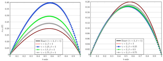
Figure 1. Numerical approximations for fixed $\beta =1$ and $\gamma =1.25,1.5,1.75,2$ (left) and fixed $\gamma =2$ and $\beta =0.25,0.5,0.75,1$ (right) in test Problem 4 with $N=10$.

Problem 5.

Let us consider the initial-value problem of Bagley–Torvik equation of fractional order with variable coefficients [24,25]

$$x^{\left(2\right)}\left(t\right)+\frac{1}{2}\sqrt{\pi }{t}^2{\mathcal{D}}_{★}^{\frac{3}{2}}x\left(t\right)-4\sqrt{t}x\left(t\right)=6t,$$

with initial conditions $x\left(0\right)=0$, $x^{\left(1\right)}\left(0\right)=0$. The exact solution is $x\left(t\right)=t^3$.

Clearly, the exact solution is a third-degree polynomial. Therefore, we take $N=3$ and $\alpha =1$, which are sufficient to get the desired approximations. Using the usual collocation points as in Problem 2 and similar to Problem 1, we get the final augmented matrix

$$\begin{array}{c}\hfill \left[\widehat{\mathit{W}};\widehat{\mathit{H}}\right]=\left[\begin{array}{cccccc}1& 1& 1& 1& ;& 0\\ -1351/585& -4782/1553& 2691/2701& 6598/129& ;& 2\\ -1277/391& -4801/882& -2659/445& 6090/97& ;& 4\\ 0& 1& 3& 6& ;& 0\end{array}\right].\end{array}$$

Solving the resulting linear system, we find

$$\mathit{A}={[-\frac{1}{3}\frac{3}{5}-\frac{1}{3}\frac{1}{15}]}^t.$$

Therefore, the approximated solution $x_{3,1}\left(t\right)$ is obtained as

$$x_{3,1}\left(t\right)=\left[11+t3t^2+3t+11+6t+15t^2+15t^3\right]\mathit{A}=t^3,$$

which is the exact solution.

Problem 6.

Consider the fractional Riccati equation [23,26]

$${\mathcal{D}}_{★}^{\gamma }x\left(t\right)+x\left(t\right)-x^2\left(t\right)=0,0<\gamma \le 1,$$

on a long time interval with $L=5$ and initial condition $x\left(0\right)=1/2$. When $\gamma =1$, the exact solution is $x\left(t\right)=\frac{1}{exp\left(t\right)+1}$.

We calculate the approximated solution $x_{N,\alpha }\left(t\right)$ using $N=7$ and $\gamma$ equals to $\alpha =1/4$. Thus, we get

$$\begin{array}{cc}\hfill & x_{7,\frac{1}{4}}\left(t\right)=0.1617950181136742t^{\frac{3}{4}}-0.03445544072182753t^{\frac{1}{2}}-0.2700823207417999t^{\frac{1}{4}}\hfill \\ \hfill & -0.009800299427063008t^{\frac{3}{2}}-0.1204495580962043t+0.04675854257899483t^{\frac{5}{4}}\hfill \\ \hfill & +0.0008798927221707359t^{\frac{7}{4}}+0.49999999999998357401.\hfill \end{array}$$

To validate this solution, we also employ the old fractional-order Bessel polynomials as well as Chelyshkov and Legendre functions from the previous works [26,27] with the same parameters as above. The corresponding solutions take the forms respectively

$$\begin{array}{cc}\hfill & x_{7,\frac{1}{4}}^B\left(t\right)=0.1617932518503192t^{\frac{3}{4}}-0.03445464899775196t^{\frac{1}{2}}-0.27008246876491873t^{\frac{1}{4}}\hfill \\ \hfill & -0.0097998224671427077t^{\frac{3}{2}}-0.1204474711992175t+0.04675716925988139t^{\frac{5}{4}}\hfill \\ \hfill & +0.00087982440038136711651t^{\frac{7}{4}}+0.5,\hfill \end{array}$$

$$\begin{array}{cc}\hfill & x_{7,\frac{1}{4}}^C\left(t\right)=0.16176395176134591t^{\frac{3}{4}}-0.034436828673633131t^{\frac{1}{2}}-0.27008706550355819t^{\frac{1}{4}}\hfill \\ \hfill & -0.0097962860256647t^{\frac{3}{2}}-0.12042146216589336t+0.046744073064058187t^{\frac{5}{4}}\hfill \\ \hfill & +0.00087942518183550405624t^{\frac{7}{4}}+0.5,\hfill \end{array}$$

$$\begin{array}{cc}\hfill & x_{7,\frac{1}{4}}^L\left(t\right)=0.16179490530760574t^{\frac{3}{4}}-0.034455365809483707t^{\frac{1}{2}}-0.2700823428770175t^{\frac{1}{4}}\hfill \\ \hfill & -0.009800287282136090t^{\frac{3}{2}}-0.12044946374788617t+0.04675849679405389t^{\frac{5}{4}}\hfill \\ \hfill & +0.00087989135193320893222t^{\frac{7}{4}}+0.49999999947316410565\hfill \end{array}$$

To further compare these collocation schemes based on various polynomials, we calculate the estimated residual errors obtained by the relation (24). The graphs of ${\mathcal{R}}_{N,\alpha }\left(t\right)$ on the interval $[0,5]$ correspond to $\gamma ,\alpha =1/4$ and for $N=7$ are shown in Figure 2. With respect to Figure 2, it is obviously seen that the residual error functions obtained by the presented Bessel-collocation method are smaller compared to the errors of other polynomial-based numerical collocation schemes.

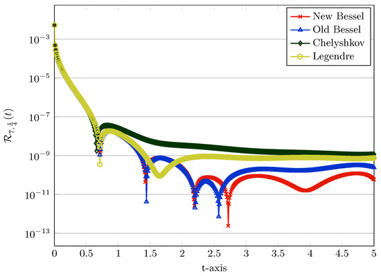
Figure 2. Comparing the error functions in test Problem 6 using old and new Bessel, Chelyshkov, and Legendre functions with $\gamma ,\alpha =1/4$, and $N=7$.

Problem 7.

Consider the following nonlinear boundary value problem with variable coefficients [6]

$$x^{\left(2\right)}\left(t\right)+\Gamma \left(\frac{4}{5}\right)\sqrt[5]{t^6}{\mathcal{D}}_{★}^{\frac{6}{5}}x\left(t\right)+\frac{11}{9}\Gamma \left(\frac{5}{6}\right)\sqrt[6]{t}{\mathcal{D}}_{★}^{\frac{1}{6}}x\left(t\right)-{[x^{\left(1\right)}\left(t\right)]}^2=2+\frac{1}{10}{t}^2,0<t<1,$$

with boundary conditions $x\left(0\right)=1$ and $x\left(1\right)=2$. The exact solution of this example is $x\left(t\right)=1+t^2$.

In this example, we have $\gamma =2$, ${\beta }_1=6/5$, and ${\beta }_2=1/6$. First, we set $\alpha =1$. The approximate solutions $x_{N,\alpha }\left(t\right)$ of Problem 7 for $N=2,3$ on $0\le t\le 1$ are obtained as follows, respectively

$$\begin{array}{cc}\hfill x_{2,1}\left(t\right)& =1.0000000000119503851t^2-2.98118\times {10}^{-11}t+1.0000000000072342687,\hfill \\ \hfill x_{3,1}\left(t\right)& =1.12820\times {10}^{-9}{t}^3+1.0000000012230527969t^2-9.66432\times {10}^{-11}t\hfill \\ \hfill & +1.0000000000012118324.\hfill \end{array}$$

To show the gain of the proposed scheme, we compare our results with the collocation method based on Bernstein operational matrix (BOM) of fractional derivative from [6]. Table 3 reports the errors in $L_{\infty }$ and $L_2$ norms of the new Bessel-collocation procedure and the errors of the BOM algorithm. This comparison shows the thoroughness of the proposed method.

Table 3. Comparison of $L_{\infty }$, $L_2$ error norms for test Problem 7.

	New Bessel		BOM [6]
	$\mathit{N}=\mathbf{2}$	$\mathit{N}=\mathbf{3}$	$\mathit{N}=\mathbf{3}$	$\mathit{N}=\mathbf{6}$	$\mathit{N}=\mathbf{12}$	$\mathit{N}=\mathbf{15}$
$L_{\infty }$	${1.06271}_{-11}$	${1.45886}_{-10}$	${3.4}_{-05}$	${1.5}_{-06}$	${5.5}_{-08}$	${1.9}_{-08}$
$L_2$	${3.00764}_{-11}$	${4.21226}_{-10}$	${2.0}_{-05}$	${7.6}_{-07}$	${2.3}_{-08}$	${7.9}_{-09}$

Problem 8.

We consider the following initial-value problem of multi-term nonlinear fractional differential equation [6]

$${\mathcal{D}}_{★}^{\gamma }x\left(t\right)+{\mathcal{D}}_{★}^{{\beta }_1}x\left(t\right)·{\mathcal{D}}_{★}^{{\beta }_2}x\left(t\right)+{[x\left(t\right)]}^2=t^6+\frac{6t^{3-\gamma }}{\Gamma (4-\gamma )}+\frac{36t^{6-{\beta }_1-{\beta }_2}}{\Gamma (4-{\beta }_1)\Gamma (4-{\beta }_2)},0<t<1,$$

where $2<\gamma <3$, $0<{\beta }_1<1$, and $1<{\beta }_2<2$ and the initial conditions are $x\left(0\right)=0$, $x^{\left(1\right)}\left(0\right)=0$, and $x^{\left(2\right)}\left(0\right)=0$. An easy calculation shows that $x\left(t\right)=t^3$ is the exact solution.

For this example, we set $\alpha =1$. By applying the collocation technique based upon new Bessel functions at C1: $(\gamma ,{\beta }_1,{\beta }_2)=(5/2,9/10,3/2)$ and for $N=3,4$, the following approximative solutions on $0\le t\le 1$ are obtained

$$\begin{array}{cc}\hfill x_{3,1}\left(t\right)& =1.0000000000004519163t^3-5.55112\times {10}^{-17}t-5.55112\times {10}^{-17},\hfill \\ \hfill x_{4,1}\left(t\right)& =8.60154\times {10}^{-13}{t}^4+0.9999999999992085443t^3-1.09400\times {10}^{-16}{t}^2\hfill \\ \hfill & -9.83260\times {10}^{-17}t+1.79230\times {10}^{-17}.\hfill \end{array}$$

A comparison between our collocation scheme at C1 and the method of shifted Jacobi operational matrix (SJOM) [6] with $N=24$ is made in Table 4. Besides the cases C1 and C2: $(\gamma ,{\beta }_1,{\beta }_2)=(2.000001,0.000009,1.000001)$, the following values of $(\gamma ,{\beta }_1,{\beta }_2)$ are used in Table 5 for comparison purposes

$$C3:(2.99,0.99,1.99),C4:(2.75,0.75,1.75),C5:(2.9999,0.9999,1.9999).$$

Table 4. Comparison of $L_{\infty }$ error norms for $\gamma =5/2$, ${\beta }_1=9/10$, ${\beta }_2=3/2$ in test Problem 8.

	New Bessel		SJOM ($\mathit{N}=24$) [6]
	$\mathit{N}=\mathbf{3}$	$\mathit{N}=\mathbf{4}$	$\mathit{\alpha },\mathit{\beta }=\mathbf{0}$	$\mathit{\alpha },\mathit{\beta }=\frac{\mathbf{1}}{\mathbf{2}}$	$\mathit{\alpha },\mathit{\beta }=\mathbf{1}$	$\mathit{\alpha },\mathit{\beta }=\frac{\mathbf{3}}{\mathbf{2}}$
$L_{\infty }$	${4.51805}_{-13}$	${6.85082}_{-14}$	${3.37}_{-05}$	${3.50}_{-05}$	${3.39}_{-05}$	${3.15}_{-05}$

Table 5. Comparison of $L_{\infty }$ error norms for various $(\gamma ,{\beta }_1,{\beta }_2)$ in test Problem 8.

	New Bessel		SJOM ($\mathit{\alpha },\mathit{\beta }=\frac{3}{2}$) [6]
Case	$\mathit{N}=3$	$\mathit{N}=4$	$\mathit{N}=4$	$\mathit{N}=8$	$\mathit{N}=16$	$\mathit{N}=24$
C2	${4.14718}_{-12}$	${3.82214}_{-15}$	${1.47}_{-09}$	${2.43}_{-10}$	${2.62}_{-11}$	${6.29}_{-12}$
C3	0	${1.87623}_{-16}$	${1.85}_{-04}$	${5.32}_{-05}$	${3.50}_{-05}$	${1.95}_{-05}$
C4	0	${3.48011}_{-14}$	${2.02}_{-03}$	${5.93}_{-04}$	${2.40}_{-04}$	${1.06}_{-04}$
C5	0	${4.49186}_{-16}$	${1.91}_{-06}$	${5.46}_{-07}$	${3.67}_{-07}$	${2.06}_{-07}$

Looking at Table 4 and Table 5 reveals that our numerical solutions obtained via novel Bessel-collocation method are in excellent agreement with the corresponding exact solutions. Moreover, our proposed scheme is superior compared to the SJOM.

Problem 9.

We consider the fractional relaxation-oscillation equation [5,6]

$${\mathcal{D}}_{★}^{\gamma }x\left(t\right)+x\left(t\right)=0,0<\gamma <2,$$

with the initial condition $x\left(0\right)=1$. If $\gamma >1$ we also have $x^{\left(1\right)}\left(0\right)=0$. The exact solution in terms of Mittag–Leffler function is given by $x\left(t\right)=E_{\gamma }(-t^{\gamma })$. Here, $E_{\gamma }\left(z\right)={\sum }_{k=0}^{\infty }\frac{z^k}{\Gamma (1+\gamma k)}$.

First, we consider $\gamma =85/100$ and set $\alpha$ equals to $\gamma$. We get the approximated solution $x_{N,\alpha }\left(t\right)$ using $N=8$ terms on $[0,1]$ as follows

$$\begin{array}{cc}\hfill & x_{8,\frac{85}{100}}\left(t\right)=0.0972690897737097t^{\frac{17}{5}}-0.0264284381134049t^{\frac{17}{4}}+0.647219778384659t^{\frac{17}{10}}\hfill \\ \hfill & -1.05749619232596t^{\frac{17}{20}}+0.00525953072336809t^{\frac{51}{10}}-0.284023703239741t^{\frac{51}{20}}\hfill \\ \hfill & -0.000568791172776014t^{\frac{119}{20}}+1.0.\hfill \end{array}$$

In Table 6, we calculate the maximum absolute errors using $N=8$ and $N=10$. In addition, a comparison is done in this table with the results obtained via SJOM [6]. Looking at Table 6 one can find that the achievement of good approximations to the exact solution is possible using only a few terms of fractional Bessel polynomials.

Table 6. Comparison of $L_{\infty }$ error norms for $\gamma ,\alpha =85/100$ in test Problem 9.

	New Bessel		SJOM ($\mathit{N}=32$) [6]
	$\mathit{N}=\mathbf{8}$	$\mathit{N}=\mathbf{10}$	$\mathit{\alpha },\mathit{\beta }=-\frac{\mathbf{1}}{\mathbf{2}}$	$\mathit{\alpha },\mathit{\beta }=\mathbf{0}$	$\mathit{\alpha },\mathit{\beta }=\frac{\mathbf{1}}{\mathbf{2}}$	$\mathit{\alpha },\mathit{\beta }=\mathbf{1}$
$L_{\infty }$	${1.01411}_{-06}$	${6.16222}_{-09}$	${5.2}_{-04}$	${8.1}_{-05}$	${1.2}_{-04}$	${2.3}_{-04}$

In the next experiments, we investigate the impact of varying $\gamma$ on the maximum absolute errors while $N=10$ is fixed. Table 7 presents the $L_{\infty }$ errors for $\gamma =0.2,0.4,0.6,0.8$ as well as $\gamma =1.2,1.4,1.6,1.8$. In all cases, we exploit $\alpha =\gamma$. Comparisons with existing approximation techniques based on operational matrix of fractional derivatives via B-spline functions [9] and shifted Jacobi functions [6] are also carried out in Table 7.

Table 7. Comparison of $L_{\infty }$ error norms for $N=10$ and various $\gamma$ in test Problem 9.

	New Bessel	B-Spline [9]	SJOM ($\mathit{N}=10$) [6]
$\mathit{\gamma }=\mathit{\alpha }$	$\mathit{N}=\mathbf{10}$	$\mathit{J}=\mathbf{8}$	$\mathit{\alpha },\mathit{\beta }=-\frac{\mathbf{1}}{\mathbf{2}}$	$\mathit{\alpha },\mathit{\beta }=\mathbf{0}$	$\mathit{\alpha },\mathit{\beta }=\frac{\mathbf{1}}{\mathbf{2}}$	$\mathit{\alpha },\mathit{\beta }=\mathbf{1}$
$0.2$	${6.71097}_{-07}$	${5.3}_{-03}$	$0.2544$	$0.1684$	$0.1824$	$0.1907$
$0.4$	${1.05544}_{-06}$	${1.9}_{-03}$	$0.1002$	$0.0363$	$0.0489$	$0.0617$
$0.6$	${3.38325}_{-07}$	${1.5}_{-03}$	$0.0314$	$0.0100$	$0.0158$	$0.0202$
$0.8$	${1.64178}_{-08}$	${1.0}_{-03}$	$0.0069$	$0.0018$	$0.0034$	$0.0045$
$1.2$	${1.53515}_{-12}$	${2.5}_{-03}$	$0.0222$	$0.0046$	$0.0046$	$0.0061$
$1.4$	${8.04611}_{-15}$	${2.4}_{-03}$	$0.0085$	$0.0014$	$0.0026$	$0.0041$
$1.6$	${6.41447}_{-16}$	−	$0.0031$	${3.8}_{-04}$	$0.0016$	$0.0029$
$1.8$	${1.17134}_{-15}$	−	$0.0012$	${7.3}_{-05}$	${9.0}_{-04}$	$0.0016$

Problem 10.

In the last case example, let us consider the following singular fractional Lane-Emden type equation [28,29]

$$\left\{\begin{array}{c}{\mathcal{D}}_{★}^{\gamma }x\left(t\right)+\frac{k}{t^{\gamma -{\beta }_1}}{\mathcal{D}}_{★}^{{\beta }_1}x\left(t\right)+\frac{1}{t^{\gamma -2}}x\left(t\right)=g\left(t\right),0<t\le 1,\hfill \\ x\left(0\right)=0,x^{\left(1\right)}\left(0\right)=0,\hfill \end{array}\right.$$

where $1<\gamma \le 2$, $0<{\beta }_1\le 1$, $k\ge 0$, and

$$g\left(t\right)=t^{2-\gamma }\left(6t\left(\frac{t^2}{6}+\frac{\Gamma (4-{\beta }_1)+k\Gamma (4-\gamma )}{\Gamma (4-{\beta }_1)\Gamma (4-\gamma )}\right)-2\left(\frac{t^2}{2}+\frac{\Gamma (3-{\beta }_1)+k\Gamma (3-\gamma )}{\Gamma (3-{\beta }_1)\Gamma (3-\gamma )}\right)\right).$$

The exact solution is $x\left(t\right)=t^3-t^2$.

To proceed, we take $\gamma =3/2$, ${\beta }_1=1/2$, and $k=2$. Using the collocation points $t_j=0.001+j/N$ for $j=0,1,\dots ,N$ and with $N=3,4$, the following approximation solutions are obtained by the Bessel-collocation procedure

$$\begin{array}{cc}\hfill & x_{3,1}\left(t\right)=1.0t^3-1.0t^2+6.23678\times {10}^{-16}t+3.40637\times {10}^{-108},\hfill \\ \hfill & x_{4,1}\left(t\right)=-2.93410\times {10}^{-15}{t}^4+1.0t^3-1.0t^2+1.28989\times {10}^{-15}t+3.06104\times {10}^{-108}.\hfill \end{array}$$

Obviously, these approximations are accurate up to machine epsilon. Table 8 reports the comparison of the absolute errors evaluated at some points $t\in [0,1]$ obtained by the Bessel-collocation method. For comparison, the results obtained by the collocation method (CM) [29] and the reproducing kernel method (RKM) [28] are also shown in Table 8. The comparisons show that the proposed method is considerably more accurate than other methods.

Table 8. Comparison of absolute errors for $\gamma =3/2,{\beta }_1=1/2$ in test Problem 10.

	New Bessel		CM [29]		RKM [28]
$\mathit{t}$	$\mathit{N}=\mathbf{3}$	$\mathit{N}=\mathbf{4}$	$\mathit{N}=\mathbf{5}$	$\mathit{N}=\mathbf{10}$	$\mathit{N}=\mathbf{5}$	$\mathit{N}=\mathbf{10}$
$0.25$	${8.25341}_{-17}$	${1.32991}_{-16}$	${1.3345}_{-03}$	${1.3232}_{-05}$	${8.7370}_{-04}$	${8.4636}_{-06}$
$0.50$	${6.41715}_{-17}$	${1.23861}_{-16}$	${1.5000}_{-03}$	${2.6000}_{-05}$	${9.9000}_{-04}$	${2.9000}_{-06}$
$0.75$	${1.37231}_{-17}$	${1.21568}_{-16}$	${5.0673}_{-03}$	${1.5634}_{-06}$	${7.6702}_{-04}$	${8.5754}_{-06}$
$1.00$	${3.40637}_{-108}$	${3.75169}_{-108}$	${3.6339}_{-03}$	${4.1443}_{-05}$	${5.4736}_{-04}$	${5.4345}_{-06}$

6. Conclusions

A practical matrix approach based on novel (orthogonal) Bessel polynomials is presented to solve multi-order fractional-order differential equations (MOFDEs). Using the matrix representations of the generalized Bessel polynomials and their derivatives with the aid of collocation points, the scheme transforms MOFDEs to a fundamental matrix equation, which corresponds to a system of (non)linear algebraic equations. To assess the efficiency and accuracy of the presented technique, several numerical examples with initial and boundary conditions are investigated. Comparisons with the exact solutions and with various alternative numerical simulations and experimental measurements have also been made. Based on the experiments, it is found that the numerical approximations are in an excellent agreement, which demonstrate the reliability and the great potential of the presented technique.

References

- Podlubny, I. Fractional Differential Equations; Academic Press: New York, NY, USA, 1999. [Google Scholar]
- El-Sayed, A.M.A.; El-Mesiry, E.M.; El-Saka, H.A.A. Numerical solution for multi-term fractional (arbitrary) orders differential equations. Comput. Appl. Math. 2004, 23, 33–54. [Google Scholar] [CrossRef]
- Edwards, J.T.; Ford, N.J.; Simpson, A.C. The numerical solution of linear multi-term fractional differential equations: Systems of equations. J. Comput. Appl. Math. 2002, 148, 401–418. [Google Scholar] [CrossRef]
- El-Sayed, A.M.A.; El-Kalla, I.L.; Ziada, E.A.A. Analytical and numerical solutions of multi-term nonlinear fractional order differential equations. Appl. Numer. Math. 2010, 60, 788–797. [Google Scholar] [CrossRef]
- Saadatmandi, A.; Dehghan, M. A new operational matrix for solving fractional-order differential equations. Comput. Math. Appl. 2010, 59, 1326–1336. [Google Scholar] [CrossRef]
- ABhrawy, H.; Taha, T.M.; Machado, J.A.T. A review of operational matrices and spectral techniques for fractional calculus. Nonlinear Dyn. 2015, 81, 1023–1052. [Google Scholar] [CrossRef]
- Talaei, Y.; Asgari, M. An operational matrix based on Chelyshkov polynomials for solving multi-order fractional differential equations. Neural Comput. Appl. 2018, 30, 1369–1376. [Google Scholar] [CrossRef]
- Izadi, M. A comparative study of two Legendre-collocation schemes applied to fractional logistic equation. Int. J. Appl. Comput. Math. 2020, 6, 71. [Google Scholar] [CrossRef]
- Lakestani, M.; Dehghan, M.; Irandoust-pakchin, S. The construction of operational matrix of fractional derivatives using B-spline functions, Commun. Nonlinear Sci. Numer. Simul. 2012, 17, 1149–1162. [Google Scholar] [CrossRef]
- Damarla, S.K.; Kundu, M. Numerical solution of multi-order fractional differential equations using generalized triangular function operational matrices. Appl. Math. Comput. 2015, 263, 189–203. [Google Scholar] [CrossRef]
- Krall, H.L.; Frink, O. A new class of orthogonal polynomials: The Bessel polynomials. Trans. Am. Math. Soc. 1949, 65, 100–115. [Google Scholar] [CrossRef]
- Han, H.; Seo, S. Combinatorial proofs of inverse relations and log-concavity for Bessel numbers. Eur. J. Combin. 2008, 29, 1544–1554. [Google Scholar] [CrossRef][Green Version]
- Yang, S.L.; Qiao, Z.K. The Bessel numbers and Bessel matrices. J. Math. Res. Exp. 2011, 31, 627–636. [Google Scholar]
- Ismail, M.E.H.; Kelker, D.H. The Bessel polynomials and the student t distribution. SIAM J. Math. Anal. 1976, 7, 82–91. [Google Scholar] [CrossRef]
- Bochner, S. Über Sturm-Liouvillesche polynomsysteme. Math. Zeit. 1929, 29, 730–736. [Google Scholar] [CrossRef]
- Grosswald, E. On some algebraic properties of the Bessel polynomials. Trans. Am. Math. Soc. 1951, 71, 197–210. [Google Scholar] [CrossRef]
- Grosswald, E. Bessel Polynomials, Lecture Notes in Math. Vol. 698; Springer: Berlin, Germany, 1978. [Google Scholar]
- Delgado, J.; Orera, H.; Pe na, J.M. Accurate algorithms for Bessel matrices. J. Sci. Comput. 2019, 80, 1264–1278. [Google Scholar] [CrossRef]
- Dehestani, H.; Ordokhani, Y.; Razzaghi, M. Fractional-order Bessel functions with various applications. Appl. Math. 2019, 64, 637–662. [Google Scholar] [CrossRef]
- Odibat, Z.; Shawagfeh, N.T. Generalized Taylor’s formula. Appl. Math. Comput. 2007, 186, 286–293. [Google Scholar] [CrossRef]
- Kazem, S.; Abbasbandy, S.; Kumar, S. Fractional-order Legendre functions for solving fractional-order differential equations. Appl. Math. Model. 2013, 37, 5498–5510. [Google Scholar] [CrossRef]
- Rehman, M.U.; Khan, R.A. A numerical method for solving boundary value problems for fractional differential equations. Appl. Math. Model. 2012, 36, 894–907. [Google Scholar] [CrossRef]
- Firoozjaee, M.A.; Yousefi, S.A.; Jafari, H.; Baleanu, D. On a numerical approach to solve multi order fractional differential equations with initial/boundary conditions. J. Comput. Nonlinear Dyn. 2015, 10, 061025. [Google Scholar] [CrossRef]
- Izadi, M.; Negar, M.R. Local discontinuous Galerkin approximations to fractional Bagley-Torvik equation. Math. Meth. Appl. Sci. 2020, 43, 4798–4813. [Google Scholar] [CrossRef]
- Wei, H.M.; Zhong, X.C.; Huang, Q.A. Uniqueness and approximation of solution for fractional Bagley-Torvik equations with variable coefficients. Int. J. Comput. Math. 2016, 94, 1541–1561. [Google Scholar] [CrossRef]
- Izadi, M. Fractional polynomial approximations to the solution of fractional Riccati equation. Punjab Univ. J. Math. 2019, 51, 123–141. [Google Scholar]
- Izadi, M. Comparison of Various Fractional Basis Functions for Solving Fractional-Order Logistic Population Model; Facta Univ. Ser. Math. Inform; University of Niš: Niš, Serbia, 2020. [Google Scholar]
- Akgul, A.; Inc, M.; Karatas, E.; Baleanu, D. Numerical solutions of fractional differential equations of Lane-Emden type by an accurate technique. Adv. Differ. Equ. 2015, 2015, 220. [Google Scholar] [CrossRef]
- Mechee, M.S.; Senu, N. Numerical study of fractional differential equations of Lane-Emden type by method of collocation. Appl. Math. 2012, 3, 851–856. [Google Scholar] [CrossRef]
© 2020 by the authors. Licensee MDPI, Basel, Switzerland. This article is an open access article distributed under the terms and conditions of the Creative Commons Attribution (CC BY) license (http://creativecommons.org/licenses/by/4.0/).