Unsupervised Anomaly Detection Approach for Time-Series in Multi-Domains Using Deep Reconstruction Error

Abstract

Automatic anomaly detection for time-series is critical in a variety of real-world domains such as fraud detection, fault diagnosis, and patient monitoring. Current anomaly detection methods detect the remarkably low proportion of the actual abnormalities correctly. Furthermore, most of the datasets do not provide data labels, and require unsupervised approaches. By focusing on these problems, we propose a novel deep learning-based unsupervised anomaly detection approach (RE-ADTS) for time-series data, which can be applicable to batch and real-time anomaly detections. RE-ADTS consists of two modules including the time-series reconstructor and anomaly detector. The time-series reconstructor module uses the autoregressive (AR) model to find an optimal window width and prepares the subsequences for further analysis according to the width. Then, it uses a deep autoencoder (AE) model to learn the data distribution, which is then used to reconstruct a time-series close to the normal. For anomalies, their reconstruction error (RE) was higher than that of the normal data. As a result of this module, RE and compressed representation of the subsequences were estimated. Later, the anomaly detector module defines the corresponding time-series as normal or an anomaly using a RE based anomaly threshold. For batch anomaly detection, the combination of the density-based clustering technique and anomaly threshold is employed. In the case of real-time anomaly detection, only the anomaly threshold is used without the clustering process. We conducted two types of experiments on a total of 52 publicly available time-series benchmark datasets for the batch and real-time anomaly detections. Experimental results show that the proposed RE-ADTS outperformed the state-of-the-art publicly available anomaly detection methods in most cases.

1. Introduction

As a result of the rapid development of computer hardware and software nowadays, time-dependent data (time-series) is being generated every minute and second. Time-series is the sequence of data points stored in timing order; each point is measured at fixed time intervals during a particular period. It is possible to extract valuable information hidden in the time-series by efficient analyses.

Anomaly detection in time-series is a significant task across many industries. An abnormal pattern that is not compatible with most of the dataset is named a novelty, outlier, or anomaly, as described in [1]. It can be caused by several reasons such as data from various classes, natural variation, data measurement, or collection errors [2]. Although anomalies can be produced through some mistakes, sometimes it indicates events like extreme weather or a considerable number of transactions. In recent years, the machine learning-based approaches have been widely used to detect unusual patterns for many application domains, for instance, the detection of malicious software and intrusions in network security systems, fault detection in manufacturing, fraud detection in finance, and disease detection in medical diagnosis.

Typically, machine-learning techniques are divided into three categories: supervised, semi-supervised, and unsupervised. If a dataset provides labels that indicate normal or abnormal, supervised techniques are used and it builds a classification model from the labeled dataset for predicting the output label of unknown data. The semi-supervised techniques use a dataset labeled as only normal or abnormal to build a classification model. However, the model may not predict correctly when the training dataset contains abnormal and normal data together. In practice, most datasets do not include labels, and unsupervised approaches are employed. The anomaly detection in time-series is the task of unsupervised learning. Currently, unsupervised anomaly detection approaches tend to detect a small number of true anomaly and a large number of false normal.

In this study, we have proposed the Reconstruction error based anomaly detection in time-series (RE-ADTS), which is the unsupervised anomaly detection approach based on the RE of the deep autoencoder model for time-series data. AE is one kind of neural network that learns to represent its input to output as the same as possible. Typically, it is used to reduce data dimensionality or to denoise noisy data. However, we additionally used the RE measurement, which is a difference between the input and its reconstructed output on the deep AE model for two purposes: measuring the anomaly and as a new feature. RE-ADTS can be summarized as follows. Foremost, it prepares subsequences based on the optimal window width that is selected using the AR model. After that, the prepared subsequences are compressed into 2-dimensional space by the deep AE model. In the anomaly detector module, first, the RE based anomaly threshold is calculated from the reconstruction errors in the compressed dataset. For batch anomaly detection, the compressed subsequences are grouped by the density-based spatial clustering of applications with noise (DBSCAN) algorithm, and the RE of each subsequence in a cluster is compared with the anomaly threshold. If most of the subsequences exceed the anomaly threshold, the cluster is considered as the anomaly. For real-time anomaly detection, the RE of the subsequence is directly compared with the anomaly threshold without the clustering process. The main contributions of this research are as follows:

• We propose the novel RE-ADTS method to detect anomalies in time-series by the unsupervised mode.
• RE-ADTS can be used in both batch and real-time anomaly detections.
• By automatically determining the window width, the RE-ADTS can be directly applied in various domains without manual configuration.
• We evaluated 10 publicly available state-of-the-art outlier detection methods on 52 benchmark time-series datasets. The RE-ADTS gave a higher performance than the compared methods in most cases.

The rest of the paper is arranged as follows. Section 2 provides an overview of related studies. The proposed approach is described in Section 3. The experimental setup is presented in Section 4. The evaluation results of the proposed method and performance comparison are provided in Section 5. The discussion part is presented in Section 6. The whole study is concluded in Section 7.

2. Related Work

Anomaly detection in time series is one of the most challenging problems in data science. As above-mentioned, we can use three different techniques for anomaly detection based on the availability of the data label. If we have a labeled dataset, it is feasible to build an accurate model using classification techniques. However, most datasets are not labeled, and the labeling process requires domain experts. Moreover, it is very time-consuming and expensive to make labels manually for the massive datasets. In this section, we introduce unsupervised anomaly detection approaches.

Distance-based techniques are widely used to detect anomalies by the unsupervised mode [3]. Ramaswamy et al. proposed an anomaly detection approach based on the k-nearest neighbor (KNN), which calculates an anomaly score for each data point by a distance between the point and the k-th nearest neighbor and orders them according to their anomaly score [4]. The first n data points from this ranking are viewed as an anomaly. Breuing et al. presented the local outlier factor (LOF) algorithm [5]; it assigns the degree of the outlier to each object depending on how they are isolated from their surrounding neighborhoods. This algorithm assumes the data distribution is spherical. However, if the data distribution is linear, the local density estimation will be incorrect [3]. He et al. [6] introduced a cluster-based local outlier factor (CBLOF) approach, where the degree of the outlier was based on the clustering technique instead of KNN. Gao et al. [7] combined the KNN with a clustering technique to detect anomalies in unlabeled telemetry data. The proposed approach initially selected a dataset near to normality using the KNN algorithm, where a point is assumed as an anomaly when its nearest neighbors in data space are far. Then, it builds a model by the single-linkage clustering algorithm from the selected dataset. For new data, it calculates the distances between the data and clusters and picks the minimum distance. If this distance is longer than the threshold, it is regarded as an anomaly. Jiang et al. [8] presented a clustering-based unsupervised intrusion detection (CBUID) algorithm that groups dataset into clusters with almost the same radius using a novel incremental clustering algorithm. These clusters are labeled as ‘normal’ or ‘attack’ based on the ratio of data points included and total points. For new data, it uses the labeled clusters as a model.

Principal component analysis (PCA) is a data transformation technique. It is commonly employed for reducing data dimension [9], but it can be used to detect anomalies. Rousseeuw et al. [10] introduced the PCA based anomaly detection approach using an orthogonal distance from the data point to the PCA subspace and score distance based on Mahalanobis distance. For normal data, both orthogonal and score distances were small. Hoffmann et al. [11] proposed a kernel-PCA for novelty detection, which is a non-linear extension of PCA. First, they mapped the input data into higher-dimensional space using the Gaussian kernel function. Then, they extracted the principal components of the data distribution, and the squared distance to the corresponding PCA subspace is used to measure novelties. Kwitt et al. proposed a robust PCA for anomaly detection and used the correlation matrix instead of the covariance matrix to calculate the principal component scores [12].

There are semi-supervised and unsupervised approaches based on the one class support vector machine (OC-SVM) proposed to detect anomalies. The unsupervised OC-SVM was first introduced by Schölkopf et al. [13] for novelty detection purposes, where the whole dataset is used to train the OC-SVM model. If the training set contains an anomaly, the learned model does not work well because the decision boundary of OC-SVM shifts toward anomalies. Amer et al. [14] presented an enhanced OC-SVM consisting of the robust OC-SVM and the eta-SVM for eliminating the previous problem. The basic idea is that anomalies contribute to the decision boundary less than normal instances.

The previously mentioned methods are also used for detecting anomalies in time-series data. Ma et al. [15] introduced OC-SVM for time-series novelty detection. In the beginning, it converts time-series into a set of vectors using the time-delay embedding process [16] and then applies the OC-SVM on these vectors. Hu et al. [17] proposed the meta-feature based OC-SVM for anomaly detection (MFAD) from time-series datasets. For the multivariate time-series, its dimension is reduced to 1-dimensional sequences using PCA or SVD techniques. Then, it extracts six meta-features from the 1-dimensional dataset and recognizes anomalies using the OC-SVM from the 6-dimensional dataset. The KNN based approach was suggested by Basu et al. [18] for cleaning noisy data from sensor signals. This method uses the median value of k number of neighborhoods of a data point and compares a difference between the median and data point to a specified threshold. However, configuring an appropriate threshold value requires knowledge about the signal.

Recently, a deep learning-based anomaly detection method for multidimensional time-series was proposed by Kieu et al. [19]. First, they presented two versions of the proposed method based on a 2-D convolutional AE and a long short term memory AE. Before detecting anomalies, it enriches the features by the statistical aspect. The difference between the enriched time-series and a reconstructed variant of this enrichment is used as an anomaly indicator. They considered the top α% (e.g., 5%) of the reconstruction error based vectors as outliers. Mohsin et al. presented a deep learning-based DeepAnT method for unsupervised anomaly detection in time-series [20]. The DeepAnT consists of two modules including a time-series predictor and anomaly detector. The time-series predictor uses a deep convolutional neural network for the time-series regression problem; the anomaly detector uses the Euclidean distance to calculate the anomaly score from the actual value and predicted value. In this research, we addressed the problem of how to detect anomalies automatically from a univariate time-series dataset without domain knowledge.

According to time-series characteristics, there are several anomaly detection techniques that are publicly available. Skyline [21] is a real-time anomaly detection system, implemented by Etsy Inc. It consists of the Horizon agent, which is responsible for collecting, cleaning, and formatting new data points and the Analyzer agent, which is responsible for analyzing every metric for the anomalies. It can be used in a large amount in a high-resolution time-series dataset because of a simple divide-and-conquer strategy.

Extensible generic anomaly detection system (EGADS) is a general time-series anomaly detection framework implemented at Yahoo [22]. This framework consists of two main components, and each of them includes several algorithms: the time-series modeling module (TMM), and the anomaly detection module (ADM). The TMM builds a model on given time-series and produces an expected value that is later consumed in the ADM to compute the anomaly score. It provides a simple mechanism to plugin new models and algorithms into the system.

Twitter Inc. introduced the AnomalyDetection open-source R package in 2015 [23]. The underlying algorithm is a seasonal hybrid ESD (S-H-ESD), which is based on the generalized extreme studentized deviate test [24] for anomalies. The Twitter anomaly detection algorithm detects anomalies from a statistical viewpoint. They implemented two variants of the anomaly detection function. The AnomalyDetectionVec is used in univariate time-series where an input is a series of values. However, if the input is a series of pairs of timestamp and value, the AnomalyDetectionTS is employed.

The Numenta anomaly detection benchmark (NAB) is an open-source framework that provides real-world time-series benchmark datasets with labeled anomalies and anomaly detectors. Numenta is the proposed anomaly detection method based on hierarchical temporal memory (HTM) in the NAB [25]. The HTM model predicts the value of the next timestamp of a given timestamp. Then, prediction error is calculated through a comparison of the predicted value and actual value. For each timestamp, it produces the likelihood, which defines how anomalous the current state is based on the prediction history of the HTM model.

3. Proposed Method

Nowadays, the usage of a deep neural network is dramatically increased in many domains such as object recognition, emotion recognition, financial anomaly detection, financial time-series prediction, and disease prediction [26,27,28]. We propose the deep learning-based anomaly detection method by extending the unsupervised novelty detection approach in [29] for time-series data. In the previous approach, the input of the deep AE model did not depend on its previous values. Moreover, the deep AE model was trained on the subset that is close to normal instead of the whole dataset. Therefore, it is not possible to use this method in time-series analysis directly, because the dataset must be in the timing order without gaps in time. The proposed approach in this study was designed to handle these problems and consists of time-series reconstructor and anomaly detector modules, as shown in Figure 1. In the time-series reconstructor module, we combined the AR model and deep AE model. AE is one type of neural network that projects its input to a lower-dimensional space and then reconstructs back it into the output. We used this characteristic of the AE model for the RE-based anomaly evaluation. In other words, when the AE model learns from the whole subsequences, the model fits more for normals than anomalies because a small ratio of the total data are anomalies. In the anomaly detector module, the density-based clustering technique with the RE based anomaly threshold was employed for batch anomaly detection. For real-time anomaly detection, only the RE based anomaly threshold was used without a clustering technique.

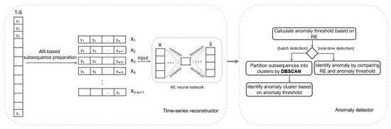
Figure 1. The general architecture of the proposed method. T-S, Time-series; AR, Autoregressive; AE, Autoencoder; RE, Reconstruction error.

For example, suppose we have a thousand series of observations in timing order. The optimal length of subsequence derived from the AR model is 15, and the number of prepared subsequences is 986. We transformed these subsequences into 2-dimensional space consisting of a latent variable (the compressed representation of subsequence) and RE (the difference between subsequence and its reconstruction) from the 15-dimensions using the deep AE model. Then, the anomaly threshold is estimated through the REs of all subsequences. For batch anomaly detection, the 2-dimensional representations of 986 subsequences are grouped based on density. As a result, assume that a total of three groups were created with subsequences of 100, 500, and 350, respectively, and 36 subsequences were not grouped. We will consider 36 unclustered subsequences as one cluster, and a total number of four clusters will be checked, whether there is an anomaly or not. Cluster 1 consisted of 100 subsequences, but the RE of 89 subsequences was higher than the anomaly threshold. For others, 5–15% of subsequences exceeded the anomaly threshold. Therefore, only subsequences in cluster 1 were tagged as anomalies. In real-time anomaly detection, the RE of each subsequence was compared with the anomaly threshold one by one without the clustering process, and all subsequences with a higher RE than the threshold were marked as an anomaly. For instance, a total of 89 subsequences will be considered as anomalies from the subsequences in cluster 1.

3.1. Autoregressive Based Deep Autoencoder Model for Time-Series Reconstruction

In this manuscript, we addressed the problem of how to detect anomalies automatically from the time-series data without domain knowledge. Therefore, the parameter configuration of our proposed model is fully automatic. The performance of time-series analysis depends on how sub-sequences are adjusted. In other words, it is critical to choose an optimal length of subsequences to obtain a higher performance in time-series analysis. However, there is no general and fixed window width for time-series data, and each time-series has its characteristics. The selection of window width is not an easy task. If the width is too large, it will increase the computation complexity and time delay by requiring more historical data for analysis. If it is too small, a time-series pattern might be lost [30]. In our proposed method, the reconstruction error of subsequences was used for anomaly detection and the subsequence consists of the value of a particular timestamp and its previous values. In other words, to determine whether a particular timestamp is an anomaly or not, we used its previous values in a subsequence. However, it requires the user to specify optimal periodicity. It is expensive to try all efficient periods one by one.

In most anomaly detection approaches, the user-defined length is used and it is not applicable when changing the dataset. The selection of window width can be solved by the approach of determining the order of the AR model. The AR model is the most successful, flexible, and easy-to-use model for the analysis of time-series. RE-ADTS prepares subsequences from the whole time-series by the sliding window method using the optimal window width. The length of the subsequence is determined through the AR model. It specifies the output value that depends linearly on its prior values. In other words, the value at the time t is dependent on values at its previous p periods, where the p is called the order. The AR model of order p can be written as [31]:

$$y_t=c+{\phi }_1{y}_{t-1}+{\phi }_2{y}_{t-2}+\dots +{\phi }_p{y}_{t-p}+{\epsilon }_t$$

(1)

where ε_t is white noise; c is a constant, φ₁–φ_p are the model parameters; and y_t−1–y_t−p are the past series values. The AR process has degrees of uncertainty; model selection methods were employed to determine the optimal window width (order p). A considerable number of model selection methods have been proposed such as cross-validation (CV), Akaike’s information criterion (AIC), Bayesian information criterion (BIC), and based on last lag (T-STAT), etc. For example, CV first randomly splits the original data into training and testing sets without overlap. Then, each candidate model is trained from the training set, and then its loss is measured from the testing set. After this procedure has been done several times, a model with the smallest loss is selected. To select the most proper window width, the commonly used approach is to fit the AR (p) model with a different number of orders p = 0. n, and choose the value of p, which minimizes some of the model selection criteria. We used several information criteria such as CV, AIC, BIC, and T-STAT [32] for the order selection.

In T-STAT, the model starts with maxlag, which is (round (12 * (number of observations/100) ** (1/4)) [33] and drops the lag until the highest lag has a t-value that is significant at the 95% level. AIC is a model selection approach proposed by Akaike [34]:

$$AI{C}_p=n\log {\widehat{e}}_p+2\mathrm{p}$$

(2)

where p is the number of order; ${\widehat{e}}_p$ is the average prediction error based on the quadratic loss; and n is the number of the sample.

BIC is another popular model selection criteria. The only difference from AIC is that the constant 2 in the AIC penalty is replaced with the logarithm of the dataset size. It selects the model that minimizes:

$$BI{C}_p=n\log {\widehat{e}}_p+p\log n$$

(3)

where p is the number of order; ${\widehat{e}}_p$ is the average prediction error based on the quadratic loss; and n is the number of the sample. The presented approach has an automated window width selection process, and it can adapt to various characteristics of time-series. Table A1 in Appendix A shows the comparison of the average f-measure on each domain using the fixed and optimal window width.

The prepared subsequences were reconstructed by the deep AE model for retrieving the reconstruction error. AE is the unsupervised learning algorithm for learning to copy its input (x₁ … x_n) to its output (y₁ … y_n) as close (x_i = y_i) as possible by reducing the distinction between inputs and outputs [35]. The architecture of AE consists of the encoder and decoder parts; both of them contain several layers with neurons. Each neuron receives an output of the activation function that converts the weighted summation of neurons in the previous layer. AE learns by changing the weights of each neuron to reduce the difference between input and its reconstructed output. The encoder part takes an input vector x and projects it into a compressed representation h called latent space. After that, the latent space is generated back to a reconstructed vector x’ in the decoder part. The following equation describes AE:

$$\begin{gathered} \mathrm{h} = \mathrm{a}\left(\mathrm{wx}+\mathrm{b}\right) \\ {\mathrm{x}}^{\prime }={\mathrm{a}}^{\prime }\left({\mathrm{w}}^{\prime }\mathrm{h}+{\mathrm{b}}^{\prime }\right) \end{gathered}$$

(4)

where a and a’ are the activation functions; w and w’ are the weight matrices; and b and b’ are the bias vectors.

The deep AE model in RE-ADTS consists of an input layer, three hidden layers, and an output layer. The number of neurons in the input and output layers are determined by the selected window width, and neurons of hidden layers will vary for each time-series dataset, depending on the number of neurons in the input layer. If the input layer has n neurons, the three hidden layers consist of n/2, 1, and n/2 neurons, respectively. The AE model reduces the dimension from n features to 1, and it is reconstructed back to the output. The layers of the encoding part use the sigmoid activation function, and the layers of the decoding part use the tanh activation function. The output of the deep AE model can be written in the vectorized form:

$$x^{\prime }= \tan \mathrm{h}\left(w^4\tan \mathrm{h}\left(w^3\mathrm{sigmoid}\left(w^2\mathrm{sigmoid}\left(w^{1}x+b^1\right)+b^2\right)+b^3\right)+b^4\right)$$

(5)

where tanh and sigmoid are the activation functions; w and b are the weight matrix and the bias vector for each layer, respectively; and x is the input vector.

Generally, AE is used for dimensionality reduction or data denoising purposes. If using AE for dimensionality reduction, the encoder part is employed and the decoder part is used to regenerate any corrupted or noisy inputs. In the RE-ADTS, a new feature is extracted using a reconstruction error that occurs to reconstruct the subsequence on the deep AE model. RE can be used to identify anomalies because some data that are different from most data give a higher RE than regular data. The RE is calculated through the mean of the squared difference between the input features and reconstructed features:

$$RE=\frac{1}{n}{\displaystyle \sum }_{i=1}^n\Vert x_i-x_i^{\prime }\Vert {}_2^2$$

(6)

where n is the number of input features; x_i is the i-th feature; and x_i’ is the reconstruction of the i-th feature. As a result of the time-series reconstructor module, there are two kinds of data generated from the subsequences using the deep AE model, and reconstruction errors and compressed representations of the subsequences are passed to the anomaly detector module for further analysis.

3.2. Reconstruction Error Based Anomaly Identification

We used the DBSCAN clustering technique with the anomaly threshold based on RE for batch anomaly detection. Before the clustering process, we reduced the dimension of subsequences into latent space using the AE model. The latent space is a compressed representation of the subsequence. Then, we added one more feature based on RE. Figure A1 in Appendix B shows the average f-measure on each domain. First, we used only latent space and RE in clustering, separately. Both the latent space and REs were not enough to use in clustering. Therefore, we combined them in the proposed method. Ester et al. introduced the DBSCAN algorithm in 1996, which separates high-density regions from one another depending on location [36]. The main advantage is that it can find arbitrarily shaped groups without requiring the number of clusters to be specified. For the unlabeled dataset, knowledge of the group quantity is unavailable. Moreover, a relatively small percentage of the total data is anomalous, and may be scattered in different locations. DBSCAN works efficiently on these arbitrary shaped clusters. There are two parameters in the DBSCAN, eps, which determines a maximum radius of the neighborhood, and minPts, which defines a minimum number of points in the specified eps radius. To discover an optimal value of the eps parameter, we applied the k-dist function that was introduced in [36]. It calculates distances from each point to its k-th nearest neighbor and sorts these distances. Then, a value that is the first sharp decreasing point is picked. For the proposed method, we fitted the eps parameter by the value of the index of 98 hundredths of the sorted list. Additionally, the DBSCAN does not provide the anomaly score as it considers unclustered points as anomalies [37]. In contrast, the RE-ADTS makes a group of the unclustered points and uses the RE-based threshold obtained from the deep AE model to identify anomalies. The commonly used Otsu [38] thresholding technique is employed to estimate the anomaly threshold from the reconstruction errors of subsequences on the deep AE model, which finds the optimal value from the distribution histogram of the data points. After the clustering process, each group is checked, whether it is an anomaly or normal. If the RE of most instances exceeds the anomaly threshold, all members in the cluster are identified as anomalies. For the real-time anomaly detection, we only used the RE based threshold on each subsequence without grouping them by the DBSCAN.

4. Experimental Study

We evaluated the RE-ADTS on the six different domains including 52 time-series benchmarks. Then, the results were compared to 10 anomaly detection methods. We conducted two types of experiments for the batch and real-time anomaly detections. Training of the AE model does not require any label and learns the data distribution, which reconstructs the time-series close to normal. Anomaly detection is one case of the class imbalance problem. Abnormal samples are usually smaller than normal ones. Therefore, the AE model is more adapted to a normal dataset than an abnormal dataset. In other words, the proposed method detects anomalies based on the data distribution of most common dataset using the AE model. Therefore, in batch anomaly detection, all the compared algorithms evaluated without the train and test split. However, real-time anomaly detection used 40% of the dataset for training and the rest of the dataset for testing.

4.1. Evaluation Metrics

The confusion matrix is used to evaluate the performance of prediction models when the data labels are available. It represents the total number of correct and incorrect predictions, and most evaluation metrics are derived from the matrix. The accuracy is the proportion of correct classifications among all classifications, which is commonly used to give an overview of classification models. However, it is not a valid measurement of performance when data are imbalanced. For the anomaly detection task, the small fraction of the total dataset is the anomaly, leading to the class imbalance problem. Therefore, we assessed the RE-ADTS and other compared methods in precision, recall, F-measure, and area under the receiver operating characteristic curve (AUC). The precision returned a positive predictive rate, and the recall gave a true positive rate. These can be defined as:

$$precision=\frac{number of true positive prediction}{total number of positive prediction}$$

(7)

$$recall=\frac{number of true positive prediction}{total number of actual positives}$$

(8)

F-measure is a combination of precision and recall, and gives the harmonic mean of them. It can be defined by:

$$F-measure=\frac{2\ast precision\ast recall}{precision+recall}$$

(9)

The AUC represents how much the model is capable of distinguishing between classes, and a high AUC indicates a good result. A receiver operating characteristic (ROC) curve is created by plotting the true positive rate (TPR) against the false positive rate (FPR). The AUC score is the area of the ROC curve that represents the probability that a randomly selected positive instance will score higher than a randomly selected negative instance [39].

4.2. Experimental Dataset

Anomalies have a distinct behavior depending on their domain. Therefore, it is significant to evaluate anomaly detection methods on many domains. The Numenta Anomaly Benchmark (NAB) is a publicly available streaming anomaly detection benchmark published by Numenta [40]. NAB consists of a variety of domains such as server network utilization, temperature sensors on industrial machines, social media activity, and contains 58 streaming files, each with 1.000–22.000 observations. All streaming files were labeled by the known root causes of the anomalies from the data provider or as a result of the well-defined NAB labeling procedure [25]. Each of the files includes pairs of timestamps and actual values, but anomaly labels are in a separate file.

4.3. Parameter Tuning for RE-ADTS

In the beginning, we selected an optimal window width using the AR model for each time-series file. The AR process has degrees of uncertainty; order selection criteria were employed to determine the optimal window width (order p). We used several information criteria such as CV, AIC, BIC, and T-STAT for the order selection. Table 1 gives the average value of the selected window width for each domain.

Table 1. The average value of the selected window width for each domain using different order selection criteria on the autoregressive model.

Time-Series	CV	AIC	BIC	T-STAT
Artificial With Anomaly	21	21	11	27
realAdExchange	23	18	14	20
realAWSCloudwatch	19	22	14	25
realKnownCause	21	24	28	33
realTraffic	19	9	4	21
realTweets	18	29	17	34

The window width can be different on each file. Table 1 simply shows the average value of each domain. For CV, we used a 5-fold time-series cross-validation approach to select the best window width for the AR model. First, several candidate AR models with different window widths between two and 30 were trained from the training set, and then the loss of these models was measured from the testing set by the root mean squared error (RMSE) measurement. After this procedure had been conducted five times, a model with the smallest average loss was selected. Belonging to the selected window width, we prepared the subsequences, and the deep AE model was trained on them to extract features to be used in the anomaly detection. The deep AE model was optimized by the Adam algorithm [41], and the learning rate was 0.001 to minimize the mean squared error. The batch size and the number of epochs were 32 and 1000, respectively. From the deep AE model, the compressed subsequences that consist of the latent space and RE are retrieved. For batch anomaly detection, these compressed subsequences were clustered by the DBSCAN algorithm; the parameter minPts was configured by three. If at least 80 percent of the subsequences exceeds the anomaly threshold, the cluster was labeled as the anomaly. For real-time anomaly detection, RE of the subsequence was compared with the anomaly threshold directly without clustering.

4.4. Parameter Tuning for the Compared Algorithms

For the Twitter anomaly detection method, we used the AnomalyDetectionVec function on benchmark datasets. This function detects one or more statistically significant anomalies from a vector of observations. We used all default parameters of this function except alpha, direction, and period. The alpha parameter defines the level of statistical significance in which to accept or reject anomalies, and it was configured at 0.05 and 0.1. The direction parameter sets the directionality of the anomalies to be detected, and we configured using the ‘both’ option in our experiment. The period parameter specifies the number of observations in the subsequence and was configured by the optimal window width from the AR model, the same as the proposed approach for each file.

For Yahoo EGADS, we ran the Olympic model and SimpleThresholdModel for time-series modeling and anomaly detection, respectively. The default values of all parameters were used except for the window size. It was configured the same as the proposed method. EGADS estimates the threshold itself and returns the timestamps of the anomaly dataset as an output.

NAB provides us with time-series benchmark datasets and anomaly detectors. The results of the implemented anomaly detection algorithms were presented in [40], who introduced their NAB score measurement for performance evaluation. However, we evaluated the anomaly detectors in the NAB framework by precision, recall, and F-measure because the NAB score does not show the real true and false detections of anomalies. We evaluated the Numenta, Skyline, Bayes ChangePoint [42], Relative Entropy [43], and Windowed Gaussian, DeepAnt algorithms with the same settings in [20,25] as they performed extensive parameter configuration for each algorithm and used the optimal values.

5. Experimental Results

We conducted two types of experiments. In the first experiment, we applied a total of eight anomaly detection algorithms on 52 time-series datasets from various domains. The precision and recall are shown in Table 2. The average performances of each domain from the results on the time-series datasets are reported in Table 3 and Table 4.

Table 2. The evaluation of the state-of-the-art algorithms and the RE-ADTS on 52 Numenta anomaly detection benchmark (NAB) time-series datasets (%). Precision and recall are described in this table.

Time-Series		Yahoo EGADS		Twitter Anomaly Detection (alpha = 0.05)		Twitter Anomaly Detection (alpha = 0.1)		Skyline		Numenta		Bayes ChangePoint		Relative Entropy		Windowed Gaussian		RE-ADTS (CV)		RE-ADTS (AIC)		RE-ADTS (BIC)		RE-ADTS (T-STAT)
		P.	R.	P.	R.	P.	R.	P.	R.	P.	R.	P.	R.	P.	R.	P.	R.	P.	R.	P.	R.	P.	R.	P.	R.
artificialWithAnomaly	art_daily_flatmiddle	0.0	0.0	9.4	9.4	9.4	9.4	0.0	0.0	13.3	0.50	7.4	0.50	37.5	2.23	0.0	0.00	10.0	0.74	7.84	4.0	0.0	0.0	8.8	0.7
	art_daily_jumpsdown	0.0	0.0	2.0	2.0	2.0	2.0	0.0	0.0	0.0	0.00	8.0	0.50	16.7	0.74	0.0	0.00	7.79	4.71	3.7	2.0	3.7	1.7	8.3	3.7
	art_daily_jumpsup	0.0	0.0	28.8	28.8	28.8	28.8	95.2	14.6	30.0	1.49	8.0	0.50	47.8	2.73	0.0	0.00	38.4	33.0	49.2	31.0	86.0	27.5	71.0	32.8
	art_daily_nojump	0.0	0.0	1.7	1.7	1.7	1.7	0.0	0.0	0.0	0.00	3.8	0.25	0.0	0.00	0.0	0.00	7.78	3.47	0.0	0.0	0.0	0.0	8.0	5.0
	art_increase_spike_density	0.0	0.0	11.7	11.7	11.7	11.7	100	0.2	6.1	0.50	10.0	0.99	0.0	0.00	0.0	0.00	12.5	7.94	11.8	23.8	11.3	26.1	11.3	26.1
	art_load_balancer_spikes	65.5	4.7	26.3	26.3	26.3	26.3	0.0	0.0	25.0	3.97	12.5	0.25	27.3	0.74	42.9	4.47	35.6	45.6	75.3	53.8	35.6	48.9	76.1	54.6
	Average	10.9	0.8	13.3	13.3	13.3	13.3	32.5	2.5	12.4	1.08	8.3	0.50	21.5	1.08	7.1	0.74	18.7	15.9	24.6	19.1	22.8	17.4	30.6	20.5
realAdExchange	exchange-2_cpc	7.7	0.6	0.0	0.0	0.0	0.0	0.0	0.0	0.0	0.0	0.0	0.0	15.4	1.23	0.0	0.0	0.0	0.0	0.0	0.0	0.0	0.0	0.0	0.0
	exchange-2_cpm	37.5	1.9	9.8	6.8	9.8	6.8	0.0	0.0	13.3	2.5	40.0	1.2	0.0	0.0	0.0	0.0	50.0	0.62	20.4	6.17	20.4	6.17	20.4	6.17
	exchange-3_cpc	36.4	5.2	21.3	8.5	21.3	8.5	0.0	0.0	12.5	2	50.0	1.3	42.9	1.96	55.6	3.27	59.5	49.0	39.5	11.1	39.5	11.1	60.2	48.4
	exchange-3_cpm	11.1	0.7	2.3	0.7	2.3	0.7	0.0	0.0	8.3	1.3	20.0	0.7	33.3	1.31	25.0	0.65	32.0	16.3	28.2	15.7	28.2	15.7	27.9	15.7
	exchange-4_cpc	30.8	2.4	28.6	4.8	28.6	4.8	0.0	0.0	21.4	1.8	16.7	1.2	75.0	1.82	33.3	1.82	51.4	32.7	33.3	12.1	33.3	12.1	34.9	32.1
	exchange-4_cpm	46.2	3.7	18.5	3	18.5	3.0	60.0	1.8	33.3	3.7	22.2	1.2	66.7	1.22	44.4	2.44	37.0	6.10	35.9	14.0	35.9	14.0	36.5	14.0
	Average	28.3	2.4	13.4	3.8	13.4	4.1	10.0	0.3	14.8	1.9	24.8	0.9	38.9	1.3	26.4	1.4	38.3	17.4	26.2	9.9	26.2	9.9	30.0	19.4
realAWSCloudwatch	ec2_cpu_utilization_5f5533	50.0	0.5	100	0.2	100	0.2	100	0.2	43.8	1.7	50.0	0.2	77.8	1.74	0.0	0.0	96.6	14.1	86.2	20.1	86.2	20.1	86.5	20.6
	ec2_cpu_utilization_24ae8d	31.8	1.7	10.4	10.4	10.4	10.4	40.0	0.5	23.5	1	23.5	1.0	33.3	0.25	11.8	0.5	18.7	9.70	28.9	3.23	28.9	3.23	28.9	3.23
	ec2_cpu_utilization_53ea38	37.1	3.2	38.9	3.5	44.4	5.0	0.0	0.0	14.3	1	18.8	0.7	50	0.75	28.6	0.5	84.3	6.72	19.2	27.1	19.2	27.1	19.2	27.1
	ec2_cpu_utilization_77c1ca	0.0	0.0	17.4	17.4	17.4	17.4	60	1.5	11.5	1.5	0.0	0.0	11.1	0.5	0.0	0.0	0.0	0.0	14.3	37.5	16.4	31.5	18.8	14.6
	ec2_cpu_utilization_825cc2	0.0	0.0	79.1	30.9	79.1	30.9	100	8.7	52.2	3.5	50.0	0.6	88.9	2.33	97.3	10.5	74.0	33.2	69.9	37.3	73.9	33.8	69.3	38.2
	ec2_cpu_utilization_ac20cd	0.0	0.0	46.2	46.2	46.2	46.2	71.4	5.0	27.3	1.5	50.0	0.2	31.6	1.49	78.1	6.2	32.7	48.6	30.4	43.7	31.4	45.7	30.4	43.7
	ec2_cpu_utilization_fe7f93_	27.0	2.5	15.4	15.3	15.4	15.3	42.1	5.9	13.5	1.2	20.0	0.5	33.3	0.74	54.5	1.48	15.3	13.0	23.4	15.8	9.52	17.8	31.5	18.5
	ec2_disk_write_bytes_1ef3de	13.9	1.1	13.3	13.3	13.3	13.3	20.9	1.9	15.4	1.3	11.8	0.4	27.3	0.63	12.9	1.9	17.1	10.7	14.2	6.98	15.1	13.5	14.4	16.7
	ec2_disk_write_bytes_c0d644	24.0	1.5	18.4	18.3	18.4	18.3	75.0	1.5	29.8	3.5	0.0	0.0	50.0	1.73	38.2	3.21	35.2	4.44	38.5	13.6	24.1	16	37.8	11.9
	ec2_network_in_5abac7	41.0	3.0	21.6	21.5	21.6	21.5	29.2	1.5	30.6	2.3	5.3	0.2	0.0	0.0	80.0	0.99	38.3	24.0	37.8	29.1	0.0	0.0	38.4	29.7
	ec2_network_in_257a54	100	1.5	18.9	18.9	18.9	18.9	100	1.2	60.0	1.5	0.0	0.0	75.0	0.74	23.8	4.01	0.0	0.0	0.0	0.0	21.2	32.7	0.0	0.0
	elb_request_count_8c0756	39.0	2.0	32.1	2.2	26.3	2.5	80.0	1.0	17.4	1	16.7	0.7	20.0	0.3	50.0	0.25	62.2	15.1	40.2	17.9	27.1	9.0	50.0	17.4
	grok_asg_anomaly	17.0	0	8.4	8.4	8.4	8.4	40.0	3.4	34.6	1.9	27.3	0.6	62.5	1.1	92.0	14.8	7.42	13.5	5.7	10.1	6.1	10.8	5.6	10.0
	iio_us-east-1_i-a2eb1cd9	0.0	0.0	32.3	15.9	32.3	16.7	0.0	0.0	0.0	0.0	0.0	0.0	0.0	0.0	0.0	0.0	0.0	0.0	18.5	4.0	35.1	15.9	37.1	10.3
	rds_cpu_utilization_cc0c53	100	0.0	32.8	32.8	32.8	32.8	100	10.9	37.5	1.5	20.0	0.2	77.8	1.8	98.0	12.4	31.5	74.8	31.7	74.9	31.8	74.9	31.7	74.9
	rds_cpu_utilization_e47b3b	22.0	0.0	7.2	7.2	7.2	7.2	100	5.7	36.4	1	50.0	0.5	87.5	1.8	66.7	0.5	71.6	13.1	56.4	13.2	0.0	0.0	57.1	14.9
	Average	31.4	1.2	30.8	16.4	30.7	16.6	59.9	3.1	28.0	1.6	22.9	0.4	45.4	0.1	45.7	3.6	36.6	17.6	32.2	22.2	26.6	22.0	34.8	22.0
realKnownCause	ambient_temperature_system_failure	89.0	9.0	0.0	0.0	0.0	0.0	0.0	0.0	20.5	1.1	0.0	0.0	11.1	0.41	0.0	0.0	48.1	14.3	40.4	20.4	43.0	19.1	40.4	20.4
	cpu_utilization_asg_misconfiguration	0.0	0.0	23.4	28.2	23.4	28.2	0.0	0.0	38.9	0.9	7.3	0.5	66.7	0.8	0.0	0.0	43.1	2.74	35.4	25.4	47.8	76.1	39.2	79.5
	ec2_request_latency_system_failure	38.0	5.0	93.3	4.0	93.3	4.0	100	1.4	47.6	2.9	28.6	0.6	100	1.45	88.9	2.4	97.0	9.54	35.6	19.9	47.8	9.6	45.6	19.7
	machine_ temperature_system_failure	100	5.0	80.0	40.4	76.2	42.0	97.0	1.4	0.0	0.0	20.0	0.0	64.3	0.79	0.0	0.0	83.4	39.2	82.5	26.4	66.6	46.4	74.8	36.6
	nyc_taxi_labeled_5	89.0	2.0	0.0	0.0	0.0	0.0	0.0	0.0	21.2	0.7	0.0	0.0	76.9	0.97	0.0	0.0	68.5	3.57	62.3	15.7	65.2	19.2	67.3	17.3
	rogue_agent_key_hold	17.0	1.0	13.3	13.2	13.3	13.2	0.0	0.0	5.26	0.5	25.0	1.1	8.33	0.53	0.0	0.0	3.43	3.68	13.8	9.0	8.6	4.8	5.8	7.4
	rogue_agent_key_updown	18.0	1.0	8.5	8.5	8.5	8.5	0.0	0.0	5.56	0.2	11.8	0.4	0.0	0.0	5.3	0.2	16.9	4.53	9.5	6.3	9.7	6.5	7.1	4.6
	Average	50.1	3.5	31.2	13.5	30.7	13.7	28.1	0.4	19.9	0.9	13.2	0.4	46.8	0.7	13.5	0.4	51.5	11.1	39.9	17.6	41.3	25.9	40.0	26.5
realTraffic	occupancy_6005	12.5	0.0	14.3	1.3	15.4	1.7	50.0	0.4	6.25	0.4	0.0	0.0	4.6	0.42	0.0	0.0	25.5	10.4	14.4	13	14.6	7.5	13.6	15.5
	occupancy_t4013	58.3	6.0	78.6	4.4	73.3	4.4	100	4.0	26.3	2.0	0.0	0.0	57.1	3.2	75.0	1.2	64.9	25.2	34.5	11.6	35.5	10.8	38.7	26.8
	speed_6005	17.6	3.0	60.0	1.3	60.0	1.3	100	1.3	17.4	1.7	33.3	0.4	28.6	0.8	50.0	0.4	16.2	5.86	27.8	8.4	26.7	8.4	30.1	14.2
	speed_7578	88.9	7.0	62.0	26.7	58.6	29.3	82.6	16.4	26.9	6.0	75.0	2.6	44.4	3.5	84.6	9.5	61.8	51.7	80.0	44.8	83.9	22.4	79.7	44.0
	speed_t4013	53.3	6.0	55.1	10.8	50.8	12.0	94.4	6.8	34.5	4.0	75.0	1.2	54.5	2.4	87.5	5.6	56.5	41.6	57.1	16.0	36.6	18.0	58.3	38.0
	TravelTime_387	28.0	3.0	24.8	24.9	24.8	24.9	50.0	7.2	14.8	1.6	0.0	0.0	50.0	1.2	8.3	0.4	30.3	9.64	32.4	14.1	30.4	9.6	32.4	14.1
	TravelTime_451	22.2	1.8	17.1	17.1	17.1	17.1	0.0	0.0	7.4	0.9	16.7	0.5	12.5	0.5	0.0	0.0	33.7	12.9	20.2	8.3	20.2	8.3	24.2	13.8
	Average	40.1	3.8	44.6	12.3	42.9	12.9	68.2	5.2	19.1	2.4	28.6	0.7	36.0	1.7	43.6	2.4	41.3	22.4	38.1	16.6	35.4	12.1	39.6	23.8
realTweets	Twitter_volume_AAPL	49.3	4.2	39.4	24.2	38.8	25.0	66.4	4.7	47.1	1	12.8	0.3	100	0.31	58.3	2.6	40.5	9.95	31.6	13.9	35.7	10.7	38.7	14.5
	Twitter_volume_AMZN	38.7	2.9	38.8	2.5	37.6	2.8	32.6	0.9	30.8	0.5	18.2	0.3	100	0.25	31.3	0.6	38.5	10.1	32.3	18.5	35.1	16.4	31.5	23.0
	Twitter_volume_CRM	68.7	3.6	53.9	8.6	52.2	9.7	73.5	1.6	50	0.5	6.38	0.2	100	0.19	83.3	0.6	55.0	18.5	38.6	24.4	41.4	22.9	40.2	24.3
	Twitter_volume_CVS	37.5	2.4	11.6	12.1	11.6	12.1	55.6	0.7	48	0.8	0.0	0.0	100	0.26	51.2	1.4	38.2	13.3	36.2	12.6	21.5	12.8	37.1	17.9
	Twitter_volume_FB	9.6	0.8	10.8	3.0	10.6	3.3	17.9	0.4	26.3	0.3	15	0.4	75.0	0.19	22.2	0.4	12.3	2.78	15.3	11.7	15.3	8.7	16.1	12.7
	Twitter_volume_GOOG	28.7	5.4	33.7	9.1	31.6	10.1	59.7	2.8	30.3	0.7	10.8	0.3	80.0	0.28	65.7	1.6	49.4	13.4	35.5	24.0	34.2	18.4	32.5	23.1
	Twitter_volume_IBM	25.7	1.6	18.1	3.6	17.8	3.7	22.4	1.1	41.7	0.6	13	0.4	62.5	0.31	34.1	0.9	18.4	4.59	18.7	16.0	18.2	14.2	18.6	16.0
	Twitter_volume_KO	33.6	2.3	22.0	6.9	21.8	7.6	42.5	2.3	28.6	0.4	2.22	0.1	50.0	0.06	36.1	1.4	18.8	5.99	17.7	9.33	17.3	7.3	17.6	9.5
	Twitter_volume_PFE	30.9	2.9	17.7	17.7	17.7	17.7	100	0.3	44.4	0.5	0.0	0.0	100	0.19	33.3	0.4	32.3	6.99	28.2	21.0	26.6	16.6	28.3	20.7
	Twitter_volume_UPS	22.5	1.5	22.6	14.5	22.6	14.5	34.3	4.4	52.7	1.8	2.17	0.1	100	0.57	47.1	3.6	23.8	5.74	23.1	19.6	23.6	9.7	21.8	26.2
	Average	34.5	2.8	26.9	10.2	26.3	10.6	50.5	1.9	40.0	0.7	8.1	0.2	86.8	0.3	46.3	1.4	32.7	9.15	27.7	17.1	26.9	13.8	28.2	18.8

Table 3. F-measure of the compared algorithms on different domains of the NAB benchmark (%).

Time-Series	Yahoo EGADS	Twitter Anomaly Detection (alpha = 0.05)	Twitter Anomaly Detection (alpha = 0.1)	Skyline	Numenta	Bayes ChangePoint	Relative Entropy	Windowed Gaussian	RE-ADTS (CV)	RE-ADTS (AIC)	RE-ADTS (BIC)	RE-ADTS (T-STAT)
artificialWithAnomaly	1.5	13.3	13.3	4.3	1.9	0.9	2	1.3	16.2	20.7	16.8	22.8
realAdExchange	4.4	5.8	5.8	0.6	3.3	1.8	2.4	2.6	21.1	14.2	14.2	22.8
realAWSCloudwatch	2.2	17.9	18.1	5.7	3	0.8	1.9	6.4	18.7	22	20.3	23.2
realKnownCause	6.4	15.5	15.6	0.8	1.7	0.7	1.4	0.7	16.5	23.7	28.5	27.9
realTraffic	6.9	15.8	16.3	9.1	4.2	1.3	3.2	4.5	28.1	22.5	17.9	29.3
realTweets	5.1	13.2	13.7	3.6	1.4	0.4	0.5	2.6	14.2	20.8	18	22.1

Table 4. AUC score of the compared algorithms on different domains of the NAB benchmark (%).

Time-Series	Yahoo EGADS	Twitter Anomaly Detection (alpha = 0.05)	Twitter Anomaly Detection (alpha = 0.1)	Skyline	Numenta	Bayes ChangePoint	Relative Entropy	Windowed Gaussian	RE-ADTS (CV)	RE-ADTS (AIC)	RE-ADTS (BIC)	RE-ADTS (T-STAT)
artificialWithAnomaly	50.4	51.8	55.0	51.3	50.4	50.1	50.5	50.3	52.6	57.5	56.0	57.3
realAdExchange	50.9	51.2	51.3	50.1	50.6	50.3	50.5	50.6	54.7	56.7	53.7	56.7
realAWSCloudwatch	47.2	55.3	55.3	51.4	50.6	50.2	50.5	51.6	56.3	51.0	50.5	51.6
realKnownCause	51.6	55.0	55.1	50.2	50.4	50.1	50.3	50.2	53.9	62.0	61.6	60.4
realTraffic	51.8	54.9	54.9	52.9	50.9	50.3	50.9	51.3	60.7	57.2	46.3	60.5
realTweets	51.1	53.3	53.3	50.8	50.3	50.1	50.1	50.6	52.3	55.5	54.7	56.1

Table 2 shows how the anomaly was detected by precision and recall measurements. From Table 2, it can be seen that most anomaly detection methods tended to detect a small proportion of the total number of anomalies, even though the precision was high. Therefore, we show a ratio between average precision and recall in each domain in Figure 2. The comparisons of average precision, recall, and AUC measurements of the compared algorithms in each domain are illustrated in Figure A2, Figure A3 and Figure A4 in Appendix C, respectively.

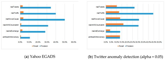
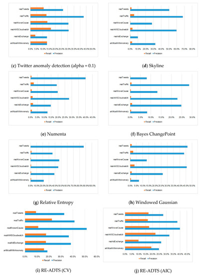
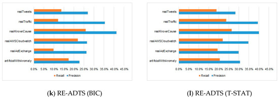
Figure 2. The proportion of precision and recall on different domains for each of the compared algorithms.

The recall is a fraction of the “true positive” predictions over the total number of the positive dataset, while the precision is a fraction of the “true positive” predictions among all positive predictions. The improvement in the recall typically degrades the precision and vice versa. It is hard to compare models with low precision along with high recall, and high precision along with low recall. Therefore, F-measure is used to evaluate recall and precision at the same time, where the highest F-measure indicates a good result. Table 3 and Table 4 show the average values of the F-measure and AUC score of the compared algorithms on six different domains in the NAB benchmark framework, and the best results are highlighted in bold.

For anomaly detection in real-time, we conducted the second experiment. In this experiment, we only used the threshold for anomaly identification without the clustering process. First, we trained the deep AE model on 40% of the whole time-series, and the rest of the dataset was used for testing; the model structure was the same as the previous experiment. We estimated the anomaly threshold from the reconstruction errors of the training dataset. For each subsequence in time-series, its RE was obtained from the trained deep AE model. Then, it was used to determine whether the subsequence was an anomaly or normal. We compared the precision, recall, and F-measure of the RE-ADTS to the evaluation of six algorithms on 20 time-series datasets in [20]. The comparison results are presented in Table 5, and the best results of F-measure are highlighted in bold.

Table 5. AUC score of the compared algorithms on different domains of the NAB benchmark.

Time-Series		ContextOSE			Numenta			NumentaTM			Skyline			Twitter Anomaly Detection			DeepAnT			RE-ADTS (T-STAT)
		P.	R.	F.	P.	R.	F.	P.	R.	F.	P.	R.	F.	P.	R.	F.	P.	R.	F.	P.	R.	F.
realAdExchange	exchange-2_cpc	0.500	0.006	0.012	0.000	0.000	0.000	0.000	0.000	0.000	0.000	0.000	0.000	0.000	0.000	0.000	0.030	0.330	0.055	0.000	0.000	0.000
	exchange-3_cpc	0.750	0.020	0.039	1.000	0.013	0.026	1.000	0.007	0.014	0.000	0.000	0.000	1.000	0.020	0.039	0.710	0.030	0.058	0.487	0.725	0.583
realAWSCloudwatch	ec2_cpu_utilization_5f5533	1.000	0.005	0.010	1.000	0.007	0.014	1.000	0.010	0.020	1.000	0.002	0.004	1.000	0.002	0.004	1.000	0.010	0.020	0.086	0.960	0.158
	rds_cpu_utilization_cc0c53	1.000	0.005	0.010	1.000	0.002	0.004	1.000	0.002	0.004	1.000	0.100	0.182	0.620	0.012	0.024	1.000	0.030	0.058	0.317	0.749	0.445
realKnownCause	ambient_temperature_system_failure	0.330	0.001	0.002	0.420	0.004	0.008	0.500	0.006	0.012	0.000	0.000	0.000	0.000	0.000	0.000	0.260	0.060	0.098	0.314	0.377	0.343
	cpu_utilization_asg_misconfiguration	0.120	0.001	0.002	0.640	0.018	0.035	0.520	0.010	0.020	0.000	0.000	0.000	0.740	0.010	0.020	0.630	0.360	0.458	0.228	0.977	0.370
	ec2_request_latency_system_failure	1.000	0.009	0.018	1.000	0.009	0.018	1.000	0.009	0.018	1.000	0.014	0.028	1.000	0.020	0.039	1.000	0.040	0.077	0.161	0.656	0.258
	machine_ temperature_system_failure	1.000	0.001	0.002	0.580	0.004	0.008	0.270	0.004	0.008	0.970	0.010	0.020	1.000	0.020	0.039	0.800	0.001	0.002	0.564	0.690	0.621
	nyc_taxi_labeled_5	1.000	0.002	0.004	0.770	0.007	0.014	0.850	0.006	0.012	0.000	0.000	0.000	0.000	0.000	0.000	1.000	0.002	0.004	0.266	0.472	0.340
	rogue_agent_key_hold	0.330	0.005	0.010	1.000	0.005	0.010	0.500	0.005	0.010	0.000	0.000	0.000	0.000	0.000	0.000	0.340	0.050	0.087	0.054	0.179	0.083
	rogue_agent_key_updown	0.000	0.000	0.000	0.140	0.002	0.004	0.000	0.000	0.000	0.000	0.000	0.000	0.110	0.002	0.004	0.011	0.001	0.002	0.119	0.045	0.066
realTraffic	occupancy_6005	0.500	0.004	0.008	0.330	0.004	0.008	0.200	0.004	0.008	0.500	0.004	0.008	0.500	0.004	0.008	0.500	0.004	0.008	0.162	0.285	0.206
	occupancy_t4013	1.000	0.008	0.016	0.400	0.008	0.016	0.660	0.008	0.016	1.000	0.040	0.077	1.000	0.020	0.039	1.000	0.036	0.069	0.328	0.492	0.394
	speed_6005	0.500	0.004	0.008	0.660	0.008	0.016	0.250	0.008	0.016	1.000	0.010	0.020	1.000	0.010	0.020	1.000	0.008	0.016	0.298	0.268	0.282
	speed_7578	0.570	0.030	0.057	0.660	0.030	0.057	0.600	0.020	0.039	0.860	0.160	0.270	1.000	0.010	0.020	1.000	0.070	0.131	0.413	0.713	0.523
	speed_t4013	1.000	0.008	0.016	1.000	0.010	0.020	0.800	0.010	0.020	1.000	0.060	0.113	1.000	0.010	0.020	1.000	0.080	0.148	0.396	0.624	0.484
	TravelTime_387	0.600	0.010	0.020	0.250	0.004	0.008	0.330	0.004	0.008	0.620	0.070	0.126	0.200	0.004	0.008	1.000	0.004	0.008	0.221	0.245	0.233
	TravelTime_451	1.000	0.005	0.010	1.000	0.005	0.010	0.000	0.000	0.000	0.000	0.000	0.000	0.000	0.000	0.000	1.000	0.009	0.018	0.000	0.000	0.000
RealTweets	Twitter_volume_GOOG	0.750	0.002	0.004	0.360	0.003	0.006	0.380	0.005	0.010	0.590	0.020	0.039	0.810	0.010	0.020	0.750	0.010	0.020	0.228	0.377	0.284
	Twitter_volume_IBM	0.370	0.002	0.004	0.150	0.002	0.004	0.220	0.005	0.010	0.220	0.010	0.019	0.500	0.009	0.018	0.500	0.005	0.010	0.196	0.269	0.227

6. Analysis and Discussion

Table 4 shows the average AUC scores of the compared algorithms on six different domains. The algorithm with a higher AUC score could distinguish anomalies and normals well. For anomaly detection problems, datasets tend to have an imbalance between the positive (anomaly) and negative (normal) samples. As we can see from Table 4, the proposed RE-ADTS gave a higher AUC score in most of the domains, but the AUC scores were very close to each other. In other words, the AUC score was insensitive to biased domains. For F-measure in the anomaly detection method, the minority class was more important than the majority class. Therefore, we assessed the experimented anomaly detection methods by precision, recall, and f-measure.

Table 2 shows the precision and recall of the compared eight algorithms on a total of 52 benchmark datasets of six domains. From the results of Table 2, we can see that the high precision was followed by the low recall. For example, the average precision of Yahoo EGADS, Skyline, Numenta, Bayes ChangePoint, Relative Entropy, and Windowed Gaussian algorithms on all six domains was between 17.6% and 45.9%; but the recall was 0.5–2.4%, 13.58–46 times lower than the precision. In consideration of the Twitter anomaly detection, the average precision in all six domains was 26.2% when the alpha parameter was 0.1, and its average recall was 11.7%. The proposed RE-ADTS presented 33.9% average precision, while the average recall was 21.8%, and was 1.55 times lower than the precision.

It can be seen from Figure 2 that the compared algorithms, except for the Twitter anomaly detection and RE-ADTS methods, showed a relatively small recall compared to their precision. In other words, most of the compared algorithms tended to detect a large number of false normals with an extremely low proportion of actual anomalies correctly. However, the RE-ADTS increased the number of true detections of anomalies.

The F-measure considers both precision and recall and provides the chance to evaluate them at the same time. Figure 3 presents the average F-measure of the analyzed algorithms on the domains of artificialWithAnomaly, realAdExchange, realTraffic, realAWSCloudwatch, realKnownCause, and realTweets. It can be regarded from Figure 3 that the proposed RE-ADTS presented the highest F-measure in all domains and was approximately 1.6–3.9 times better than the best performing algorithms in these domains. For Twitter anomaly detection, the alpha parameter did not influence the performance and showed better results than the other compared algorithms except for the RE-ADTS.

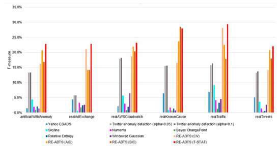
Figure 3. The performance comparison of the analyzed anomaly detection methods on different domains.

In real-time anomaly detection, we used only 40% of the dataset to train the deep AE model for estimation of the reconstruction error based anomaly threshold. Although the proposed anomaly detection approach was based on deep learning, it is not data-hungry. In Table 4, the average precision of the compared algorithms was between 0.48 and 0.7, but the average recall was 0.006–0.062, whereas the proposed RE-ADTS reached better recall with the precision of 0.241, and its F-measure outperformed in 16 of 20 datasets.

7. Conclusions

In this study, we proposed the unsupervised RE-ADTS approach based on deep learning for detecting anomalies in time-series datasets. The RE-ADTS can adapt to different domains because it automatically adjusts the optimal values of used parameters such as the window width for subsequence preparation using the AR model, RE based anomaly threshold using the Otsu thresholding method, and the maximum radius of the neighborhood (eps) of the DBSCAN using the k-dist function. Moreover, it is available to detect batch and real-time anomalies. For batch anomaly detection, we combined (1) the AR model for the optimal window width; (2) deep AE model for the anomaly threshold and dimensionality reduction; and (3) DBSCAN clustering algorithm. Clustering techniques divide the dataset into groups by their similarity. Accordingly, if most of the subsequences in the same cluster are an anomaly, all subsequences in this cluster are expressed equally as anomalies. We conducted two types of experiments for batch and real-time anomaly detections. In batch anomaly detection, we evaluated eight anomaly detection algorithms on 52 time-series datasets from six domains of the NAB benchmark framework. The experimental results showed that the RE-ADTS outperformed the compared methods by F-measure and AUC score in most domains. For the real-time anomaly detection, we only applied the anomaly threshold from the deep AE model without cluster analysis. We used 40% of the dataset for training and 60% for testing. Based on precision, recall, and F-measure, the proposed approach outperformed in 16 of 20 benchmark datasets. The anomaly detection problem is one kind of class imbalance problem. In our experimental study, the imbalance ratio of our datasets was between 8 and 10. Even though we trained the proposed AE model from the all data, it learnt more normals than anomalies, and its results outperformed the compared algorithms. In this research, we leave the problem of imbalance ratio as future work.

References

- Chandola, V.; Banerjee, A.; Kumar, V. Anomaly detection: A survey. ACM Comput. Surv. 2009, 41, 1–58. [Google Scholar] [CrossRef]
- Tan, P.N.; Steinbach, M.; Kumar, V. Anomaly Detection. In Introduction to Data Mining; Goldstein, M., Harutunian, K., Smith, K., Eds.; Pearson Education, Inc.: Boston, MA, USA, 2006; pp. 651–680. [Google Scholar]
- Goldstein, M.; Uchida, S. A comparative evaluation of unsupervised anomaly detection algorithms for multivariate data. PLoS ONE 2016, 11, e0152173. [Google Scholar] [CrossRef]
- Ramaswamy, S.; Rastogi, R.; Shim, K. Efficient algorithms for mining outliers from large data sets. In Proceedings of the 2000 ACM SIGMOD International Conference on Management of Data, Dallas, TX, USA, 16–18 May 2000. [Google Scholar]
- Breunig, M.M.; Kriegel, H.P.; Ng, R.T.; Sander, J. LOF: Identifying density-based local outliers. In Proceedings of the 2000 ACM SIGMOD International Conference on Management of Data, Dallas, TX, USA, 16–18 May 2000. [Google Scholar]
- He, Z.; Xu, X.; Deng, S. Discovering cluster-based local outliers. Pattern Recognit. Lett. 2003, 24, 1641–1650. [Google Scholar] [CrossRef]
- Gao, Y.; Yang, T.; Xu, M.; Xing, N. An unsupervised anomaly detection approach for spacecraft based on normal behavior clustering. In Proceedings of the Fifth International Conference on Intelligent Computation Technology and Automation, Zhangjiajie, China, 12–14 January 2012. [Google Scholar]
- Jiang, S.; Song, X.; Wang, H.; Han, J.J.; Li, Q.H. A clustering-based method for unsupervised intrusion detections. Pattern Recognit. Lett. 2006, 27, 802–810. [Google Scholar] [CrossRef]
- Li, M.; Yu, X.; Ryu, K.H.; Lee, S.; Theera-Umpon, N. Face recognition technology development with Gabor, PCA and SVM methodology under illumination normalization condition. Clust. Comput. 2018, 21, 1117–1126. [Google Scholar] [CrossRef]
- Rousseeuw, P.J.; Hubert, M. Anomaly detection by robust statistics. Data Min. Knowl. Discov. 2018, 8, e1236. [Google Scholar] [CrossRef]
- Hoffmann, H. Kernel PCA for novelty detection. Pattern Recognit. 2018, 40, 863–874. [Google Scholar] [CrossRef]
- Kwitt, R.; Hofmann, U. Robust methods for unsupervised PCA-based anomaly detection. In Proceedings of the IEEE/IST Workshop on Monitoring, Attack Detection and Mitigation, Tuebingen, Germany, 28–29 September 2006. [Google Scholar]
- Schölkopf, B.; Williamson, R.; Smola, A.; Shawe-Taylor, J.; Platt, J. Support Vector Method for Novelty Detection. Adv. Neural Inf. Process. Syst. 2000, 12, 582–588. [Google Scholar]
- Amer, M.; Goldstein, M.; Abdennadher, S. Enhancing One-class Support Vector Machines for Unsupervised Anomaly Detection. In Proceedings of the ACM SIGKDD Workshop on Outlier Detection and Description, Chicago, IL, USA, 1 August 2013. [Google Scholar]
- Ma, J.; Perkins, S. Time-series novelty detection using one-class support vector machines. In Proceedings of the International Joint Conference on Neural Networks, Portland, OR, USA, 20–24 July 2003. [Google Scholar] [CrossRef]
- Packard, N.H.; Crutchfield, J.P.; Farmer, J.D.; Shaw, R.S. Geometry from a time series. Phys. Rev. Lett. 1980, 45, 712. [Google Scholar] [CrossRef]
- Hu, M.; Ji, Z.; Yan, K.; Guo, Y.; Feng, X.; Gong, J.; Dong, L. Detecting anomalies in time series data via a meta-feature based approach. IEEE Access 2018, 6, 27760–27776. [Google Scholar] [CrossRef]
- Basu, S.; Meckesheimer, M. Automatic outlier detection for time series: An application to sensor data. Knowl. Inf. Syst. 2007, 11, 137–154. [Google Scholar] [CrossRef]
- Kieu, T.; Yang, B.; Jensen, C.S. Outlier detection for multidimensional time series using deep neural networks. In Proceedings of the 19th IEEE International Conference on Mobile Data Management (MDM), Aalborg, Denmark, 26–28 June 2018. [Google Scholar]
- Munir, M.; Siddiqui, S.A.; Dengel, A.; Ahmed, S. Deepant: A deep learning approach for unsupervised anomaly detection in time series. IEEE Access 2018, 7, 1991–2005. [Google Scholar] [CrossRef]
- Skyline. Available online: https://github.com/etsy/skyline (accessed on 26 November 2019).
- Laptev, N.; Amizadeh, S.; Flint, I. Generic and scalable framework for automated time-series anomaly detection. In Proceedings of the 21th ACM SIGKDD International Conference on Knowledge Discovery and Data Mining, Sydney, Australia, 10–13 August 2015. [Google Scholar]
- AnomalyDetection R package. Available online: https://github.com/twitter/AnomalyDetection (accessed on 26 November 2019).
- Rosner, B. Percentage points for a generalized ESD many-outlier procedure. Technometrics 1983, 25, 165–172. [Google Scholar] [CrossRef]
- Ahmad, S.; Lavin, A.; Purdy, S.; Agha, Z. Unsupervised real-time anomaly detection for streaming data. Neurocomputing 2017, 262, 134–147. [Google Scholar] [CrossRef]
- Amarbayasgalan, T.; Lee, J.Y.; Kim, K.R.; Ryu, K.H. Deep Autoencoder Based Neural Networks for Coronary Heart Disease Risk Prediction. In Heterogeneous Data Management, Polystores, and Analytics for Healthcare; Springer: Los Angeles, CA, USA, 2019; Volume 11721, pp. 237–248. [Google Scholar]
- Batbaatar, E.; Li, M.; Ryu, K.H. Semantic-Emotion Neural Network for Emotion Recognition from Text. IEEE Access 2019, 7, 111866–111878. [Google Scholar] [CrossRef]
- Munkhdalai, L.; Munkhdalai, T.; Park, K.H.; Amarbayasgalan, T.; Erdenebaatar, E.; Park, H.W.; Ryu, K.H. An End-to-End Adaptive Input Selection with Dynamic Weights for Forecasting Multivariate Time Series. IEEE Access 2019, 7, 99099–99114. [Google Scholar] [CrossRef]
- Amarbayasgalan, T.; Jargalsaikhan, B.; Ryu, K.H. Unsupervised novelty detection using deep autoencoders with density based clustering. Appl. Sci. 2018, 8, 1468. [Google Scholar] [CrossRef]
- Kraslawski, A.; Turunen, I. European Symposium on Computer Aided Process Engineering-13: 36th European Symposium of the Working Party on Computer Aided Process Engineering; Elsevier: Oxford, UK, 2003; pp. 462–463. [Google Scholar]
- Autoregressive Model. Available online: https://en.wikipedia.org/wiki/Autoregressive_model (accessed on 26 November 2019).
- Akaike, H. A new look at the statistical model identification. IEEE Trans. Autom. Control 1974, 19, 716–723. [Google Scholar] [CrossRef]
- Statsmodels. Available online: https://www.statsmodels.org/stable/generated/statsmodels.tsa.ar_model.AR.fit.html (accessed on 7 July 2020).
- Ding, J.; Tarokh, V.; Yang, Y. Model selection techniques: An overview. IEEE Signal Process. Mag. 2018, 35, 16–34. [Google Scholar] [CrossRef]
- Kim, H.; Hirose, A. Unsupervised Fine Land Classification Using Quaternion Autoencoder-Based Polarization Feature Extraction and Self-Organizing Mapping. IEEE Trans. Geosci. Remote Sens. 2017, 56, 1839–1851. [Google Scholar] [CrossRef]
- Ester, M.; Kriegel, H.P.; Sander, J.; Xu, X. A Density-Based Algorithm for Discovering Clusters in Large Spatial Databases with Noise. In Proceedings of the Second International Conference on Knowledge Discovery and Data Mining, Portland, OR, USA, 2–4 August 1996. [Google Scholar]
- Jin, C.H.; Na, H.J.; Piao, M.; Pok, G.; Ryu, K.H. A Novel DBSCAN-based Defect Pattern Detection and Classification Framework for Wafer Bin Map. IEEE Trans. Semicond. Manuf. 2019, 32, 286–292. [Google Scholar] [CrossRef]
- Otsu, N. A Threshold Selection Method from Gray-Level Histograms. IEEE Trans. Syst. Man Cybern. 1979, 9, 62–66. [Google Scholar] [CrossRef]
- Hanley, J.A.; McNeil, B.J. The meaning and use of the area under a receiver operating characteristic (ROC) curve. Radiology 1982, 143, 29–36. [Google Scholar] [CrossRef] [PubMed]
- Home of the HTM Community. Available online: https://www.numenta.org/ (accessed on 26 November 2019).
- Kingma, D.P.; Ba, J. Adam: A method for stochastic optimization. In Proceedings of the 3rd International Conference for Learning Representations, San Diego, CA, USA, 7–9 May 2014. [Google Scholar]
- Adams, R.P.; MacKay, D.J. Bayesian online changepoint detection. arXiv 2017, arXiv:0710.3742. [Google Scholar]
- Wang, C.; Viswanathan, K.; Choudur, L.; Talwar, V.; Satterfield, W.; Schwan, K. Statistical techniques for Online Anomaly Detection in Data Centers. In Proceedings of the 12th IFIP/IEEE International Symposium on Integrated Network Management (IM 2011) and Workshops, Dublin, Ireland, 23–27 May 2011. [Google Scholar]
© 2020 by the authors. Licensee MDPI, Basel, Switzerland. This article is an open access article distributed under the terms and conditions of the Creative Commons Attribution (CC BY) license (http://creativecommons.org/licenses/by/4.0/).