An Analytical Method for the Determination of Temperature Distribution in Short Journal Bearing Oil Film

Abstract

The aim of this paper is to derive an equation for the temperature distribution in journal bearing oil film, in order to predict the thermal load of a bearing. This is very important for the prevention of critical regimes in a bearing operation. To achieve the goal, a partial differential equation of the temperature field was first derived, starting from the energy equation coupled with the Reynolds equation of hydrodynamic lubrication for a short bearing of symmetric geometry. Then, by solving the equation analytically, the function of temperature distribution in the bearing oil film has been obtained. The solution is applied to the journal bearing, for which the experimental data are available in the references. Finally, the obtained results have been compared to the corresponding experimental values for two operating regimes, and a good level of agreement was achieved.

1. Introduction

Journal bearings are some of the oldest and most relevant machine elements. When it comes to the design, the concept of these bearings did not significantly change over the course of history, retaining its original simplicity and functionality. However, as the needs of mankind grew, machines were becoming more and more complex, and they were working in increasingly difficult conditions. To keep the bearing operation reliable even in such conditions, the materials of the bearings and their lubricants were improved over time. The bearing materials were changed in terms of improving their slip properties and embeddability, and the lubricants were changed in terms of improving their rheological properties. These improvements are the result of the studies of many researchers.

The most significant discoveries in the field of journal bearings were made by three researchers: N. P. Petrov, B. Tower and O. Reynolds [1], who recognized and formulated the phenomenon of hydrodynamic lubrication independently of each other. In the hydrodynamic lubrication regime of a journal bearing, the journal and its housing are separated by a thin layer of oil, and the friction and wear are minimized. Viscous friction of the oil causes heat generation, which in certain conditions can significantly worsen the performance of the bearing. A higher temperature of the oil film reduces the load carrying capacity of the bearing due to decrease of the oil film stiffness. In extreme cases, this can lead to a seizure of the bearing due to the rupture of the oil film, when "welding" takes place at the contact points of micro-irregularities. For this reason, the need for knowing the distribution of temperature in the lubricant is imposed as an imperative, in order to prevent the aforementioned negative phenomena. Furthermore, knowing the temperature of the oil film can also be helpful when selecting the journal and bearing materials.

The first research on thermal effects in journal bearings was conducted by American engineer Albert Kingsbury and his study of lubrication (1933). In the study, he showed that there were significant differences between theoretical and experimental results regarding the load carrying capacity of the hydrodynamic bearing. The differences appeared since the heat generated by viscous friction was neglected in the previous theoretical research [2]. According to some researchers, the generated heat can reduce the load carrying capacity up to two times [3,4].

To describe the thermal phenomena in hydrodynamic lubrication theory, different methods have been developed. Due to their simplicity and efficiency, adiabatic methods [5] occupy a significant place among these methods, and according to adiabatic methods there is no thermal interaction between the oil film and the surrounding bearing structure. In other words, all the heat generated in the oil film is transported away by convection, i.e., together with the oil flowing out of the bearing sides.

One of the simplest adiabatic methods is the effective viscosity method [2,3,5,6,7,8,9], which yields acceptable results in a limited range of the bearing operation regime [2,6,7]. According to this method, the concept of effective viscosity, which corresponds to an average temperature value in the oil film (effective temperature), is introduced. The average temperature is calculated in an iterative manner based on the equations of global energy balance for the oil film, using the appropriate viscosity-temperature functional dependence. The oil film temperature determined in this way is a measure of thermal load of the bearing.

A more general and more complex adiabatic method is Cope’s adiabatic method [2,5,10], in which the central place is occupied by Cope’s adiabatic energy equation and Reynolds equation of hydrodynamic lubrication. Cope’s adiabatic energy equation describes temperature field in the oil film of the journal bearing. The equation is a special case of a general energy equation, which neglected solid body heat conduction. The Reynolds equation describes the pressure field in the oil film of the journal bearing. In these equations, the temperature and pressure variations across the film thickness are neglected, so the system of equations becomes two-dimensional. Neither the energy equation nor Reynolds equations can be solved in analytical form. Therefore, they must be transformed into appropriate forms, in order to find their solution.

Solving the energy and Reynolds equations can be simplified using Couette method [5]. According to this method, the pressure gradients in the modified energy equation are neglected, and a simpler energy equation is obtained so that it can be easily integrated.

Many researchers dealt with various problems related to the operation of journal bearings under thermo-hydrodynamic lubrication conditions, using different forms of energy and Reynolds equations. Stokes and Ettles [11] determined the temperature field in the oil and bearing material by simultaneously solving the Reynolds and energy equations in the oil film, the Laplace equation in the bearing material and the oil-mixing conditions at inlet, using the numerical finite difference method. The same equations are numerically solved by Fillon and Bouyer [12], who investigated the influence of journal bearing wear on its thermo-hydrodynamic performance in terms of hydrodynamic pressure, temperature distributions at the film/bush interface, oil flow rate, power losses and thickness of the oil film. Sehgal et al. [13] also used the finite difference method while solving the Reynolds and energy equations simultaneously for the purpose of a comparative theoretical analysis of thermal behaviour of three different types of journal bearing configurations: circular, axial groove and off-set halves. Banwait and Chandrawatt [14] solved the Reynolds, energy and heat conduction equations for fluid, journal and bush temperatures using numerical methods (Finite Element Method and Finite Difference Method) with the aim to investigate the influence of different boundary conditions on the accuracy of the obtained solutions, comparing them with temperatures measured on the inner surface of the bush. In reference [15], the numerical solution of Reynolds equation and energy equation has been carried out for an elliptic bore journal bearing to outline the temperature profile, with the energy equation solved adiabatically. A comparison is then made with the circular case to analyse the effect of this irregularity. Moreno et al. [16] transformed Reynolds equation, the energy equation, and the diffusion equation for the bearing into the corresponding finite difference equations. In order to solve these equations, they developed their own model based on an analogy with the electrical circuit. Pierre et al. [17] carried out a thermo-hydrodynamic analysis of a misaligned journal bearing to predict the size of the misalignment, pressure and temperature under steady-state conditions. The analysis is based on the numerical solution of Reynolds equation, the energy equation, and Laplace heat conduction equation for the bush material. Chauhan et al. [18] conducted a thermo-hydrodynamic analysis of an elliptical journal bearing for three different grade oils in order to determine which of them is most resistant to thermal degradation. The parameters for evaluating this degradation were oil pressure, oil temperature and load carrying capacity of the bearing. These parameters were determined by solving the Reynolds equation, the energy equation, and Laplace heat conduction equation for the bush material numerically. The reference [19] presents a model for pressure and temperature calculations in a journal bearing both for the steady and the time-dependent case, taking into account shaft and bushing thermal exchange with the external environment. While solving the problem, different numerical methods were used: the finite element method, the finite difference method, and the boundary elements method. Kornaev et al. developed a computational model of a plain fluid-film bearing with means to create artificial thermal and viscosity wedge effect. The model is based on the generalized Reynolds equation and the energy equation that are solved simultaneously using finite difference method combined with the iteration procedure [20]. Babin et al. investigated the possibility of controlled lubrication principles application and presented a complex mathematical model of an active thrust fluid-film bearing with a central feeding orifice. The model incorporates the Reynolds equation and the adiabatic energy equation, which are solved numerically using finite difference method [21]. Li et al. investigated the characteristics of water-lubricated conical hydrodynamic and hybrid bearings numerically solving the generalized Reynolds’ equation and energy equation with enthalpy, and considered the effects of the gas–liquid two phases turbulence temperature, and axial flow [22].

In all the above-mentioned studies, the thermo-hydrodynamic lubrication equations are solved using different numerical methods, which can be time consuming and very demanding in terms of computer resources engagement. This can be a serious disadvantage if the real-time monitoring of a machine is necessary for diagnostic reasons. In such situations, it would be convenient to have an analytical solution for the temperature field in the oil film of the journal bearing, which could help faster diagnosis of the bearing condition. This motivated the authors of the paper to give their contribution in solving the problem. To that end, they derived an analytic expression for a two-dimensional temperature field in a journal bearing, solving simultaneously the adiabatic energy equation with a simplified Reynolds equation for a short bearing. As a criterion for assessing whether a bearing is long or short, the slenderness ratio (bearing length / bearing diameter) is used. If the ratio is greater than 2, the bearing is long, and if it is less than 1, the bearing is short [23,24]. Reynolds equation for a short bearing is a good approximation of the two-dimensional Reynolds equation if the slenderness ratio is less than 1. Since the slenderness ratio of modern bearings generally lies in the range between 0.5 and 1 [23,24], the temperature distribution equation for a short bearing would be applicable to most of the bearings currently used.

In order for the oil film temperature distribution equation to be derived analytically, it was necessary to simplify the problem by introducing a number of assumptions. For the sake of the reader, all the assumptions are listed below:

• The oil is an incompressible Newtonian fluid.
• There is no slip of the oil at the boundaries.
• The oil film thickness is small compared with the other dimensions.
• Pressure and temperature are constant through the thickness of the oil film.
• Circumferential pressure gradient in the oil film is neglected.
• The oil viscosity and specific heat are constant.
• There is no thermal interaction between the oil film and the surrounding bearing structure.
• The bearing is operating under steady-state conditions (journal speed and bearing load are constant).
• The structural components of the bearing are rigid and smooth.
• There is no misalignment in the bearing structure.
• The oil supply is not taken into account.
• No asperity contacts between the journal and the bearing.
• The bearing geometry is symmetric.
• The oil flow is laminar.

The rest of the paper is structured as follows. In Section 2, the initial equations are given for solving the temperature field problem in a journal bearing. Section 3 describes the procedure of how to derive and solve the differential equation of the temperature field for a short bearing. Section 4 contains the presentation and discussion of the results obtained after the derived equation is applied on a particular journal bearing. The conclusions of the research are given in Section 5.

2. Governing Equations

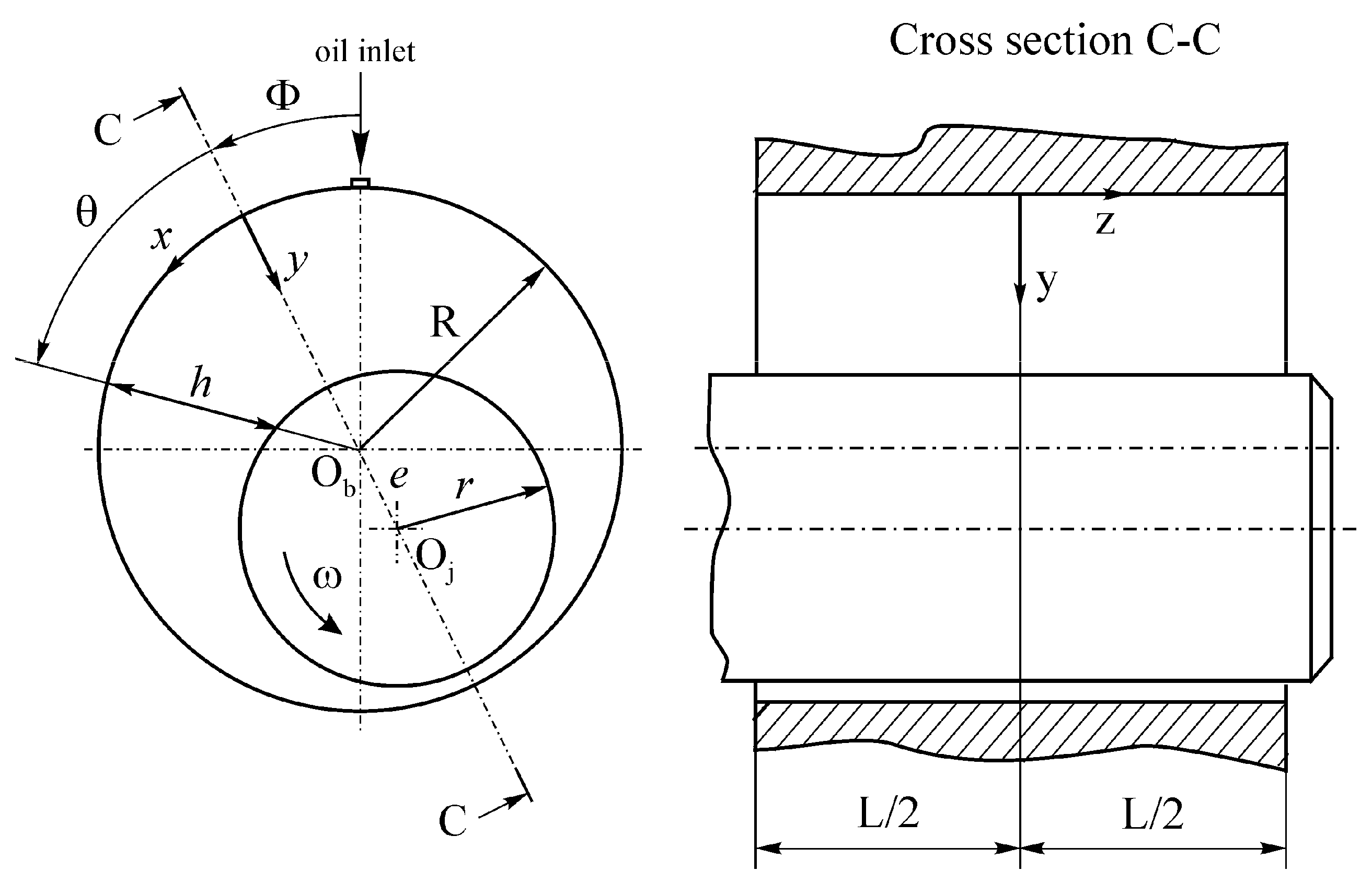
In a bearing bush with the length $L$ and the radius $R$, a journal of the radius $r$ performs rotational movement with the constant angular velocity $\omega$ under hydrodynamic lubrication conditions, as shown in Figure 1.

Figure 1. Schematics of plain journal bearing with basic parameters.

Hydrodynamic lubrication in steady-state conditions for an incompressible fluid, is described by Reynolds equation of form [5,8].

$$\frac{\partial }{\partial x}\left(\frac{h^3}{\eta }\frac{\partial p}{\partial x}\right)+\frac{\partial }{\partial z}\left(\frac{h^3}{\eta }\frac{\partial p}{\partial z}\right)=6U\frac{dh}{dx},$$

(1)

where

• $x$—streamwise coordinate direction,
• $\theta$—angular coordinate,
• $z$—axial coordinate direction,
• $p$—pressure in an arbitrary point ($x$,$z$),
• $\eta$—oil viscosity,
• $U=R\omega$—sliding velocity,
• $h=c\left(1+\epsilon \cdot \cos \theta \right)$—oil film thickness,
• $c$—radial clearance,
• $\epsilon =e/c$—eccentricity ratio,
• $\Phi =\arctan \cdot (\pi \cdot {(1-{\epsilon }^2)}^{1/2}/4\epsilon )$—attitude angle
• $e$—eccentricity ($e=\overline{O_b{O}_j}$)

Energy balance of oil film in the bearing, assuming there is no heat exchange with the mating surfaces, is described by the adiabatic energy equation of the form [5]

$$\rho c_p\left(u\frac{\partial T}{\partial x}+w\frac{\partial T}{\partial z}\right)=\eta \left[{\left(\frac{\partial u}{\partial y}\right)}^2+{\left(\frac{\partial w}{\partial y}\right)}^2\right],$$

(2)

where

• $\rho$—density of oil
• $c_p$—specific heat at constant pressure
• $T$—oil film temperature
• $u$—circumferential velocity
• $w$—axial velocity
• $y$—cross-film coordinate direction.

In order to determine the temperature field in the oil film, it is convenient to transform the Equation (2) to a form containing pressure gradients, i.e.,

$$6U\rho c_{p}h\left[\left(1-\frac{h^2}{6\eta U}\frac{\partial p}{\partial x}\right)\left(\frac{\partial T}{\partial x}\right)-\frac{h^2}{6\eta U}\frac{\partial p}{\partial z}\left(\frac{\partial T}{\partial z}\right)\right]=\frac{12\eta U^2}{h}\left\{1+\frac{h^4}{12{\eta }^2{U}^2}\left[{\left(\frac{\partial p}{\partial x}\right)}^2+{\left(\frac{\partial p}{\partial z}\right)}^2\right]\right\},$$

(3)

the derivation procedure of which is provided in Appendix A.

In order to solve Equations (1) and (3), they need to be converted into a dimensionless form. For that purpose, the appropriate dimensionless variables $\theta$, $z{}^{\ast }$, $\lambda$, $h{}^{\ast }$, $p{}^{\ast }$ and $T{}^{\ast }$ are introduced according to the expressions:

$$\theta =\frac{x}{R},z{}^{\ast }=\frac{2z}{L},\lambda =\frac{L}{2R},h{}^{\ast }=\frac{h}{c},p{}^{\ast }=p\frac{{\left(c/R\right)}^2}{6\eta \omega },T{}^{\ast }=T\frac{\rho c_p}{\eta \omega }.$$

(4)

Bearing in mind the dimensionless variables from the Equation (4), the Equations (1) and (3) become

$$\frac{\partial }{\partial \theta }\left({\left(h{}^{\ast }\right)}^3\frac{\partial p{}^{\ast }}{\partial \theta }\right)+\frac{1}{{\lambda }^2}\frac{\partial }{\partial z{}^{\ast }}\left({\left(h{}^{\ast }\right)}^3\frac{\partial p{}^{\ast }}{\partial z{}^{\ast }}\right)=\frac{dh{}^{\ast }}{d\theta },$$

(5)

$$\left(1-{\left(h{}^{\ast }\right)}^2\frac{\partial p{}^{\ast }}{\partial \theta }\right)\frac{\partial T{}^{\ast }}{\partial \theta }-\frac{{\left(h{}^{\ast }\right)}^2}{\lambda {}^2}\frac{\partial p{}^{\ast }}{\partial z{}^{\ast }}\frac{\partial T{}^{\ast }}{\partial z{}^{\ast }}=2\frac{{\left(R/c\right)}^2}{{\left(h{}^{\ast }\right)}^2}+6{\left(R/c\right)}^2{\left(h{}^{\ast }\right)}^2\left[{\left(\frac{\partial p{}^{\ast }}{\partial \theta }\right)}^2+\frac{1}{\lambda {}^2}{\left(\frac{\partial p{}^{\ast }}{\partial z{}^{\ast }}\right)}^2\right],$$

(6)

respectively.

The dimensionless parameter $\lambda$, defined in the Equation (4), is called the slenderness ratio and is the criterion for estimating the length of the journal bearing. If it is greater than 2, then the bearing is long, and if it is less than 1, the bearing is short [23,24]. As most journal bearings in engineering applications belong to short bearings, the focus will be directed to such bearings only. In the case of a short bearing, the circumferential pressure gradient can be neglected in comparison with the axial pressure gradient. This assumption enables the coupled Equations (5) and (6) to be solved for a short bearing, in order to determine the temperature field in the bearing oil film.

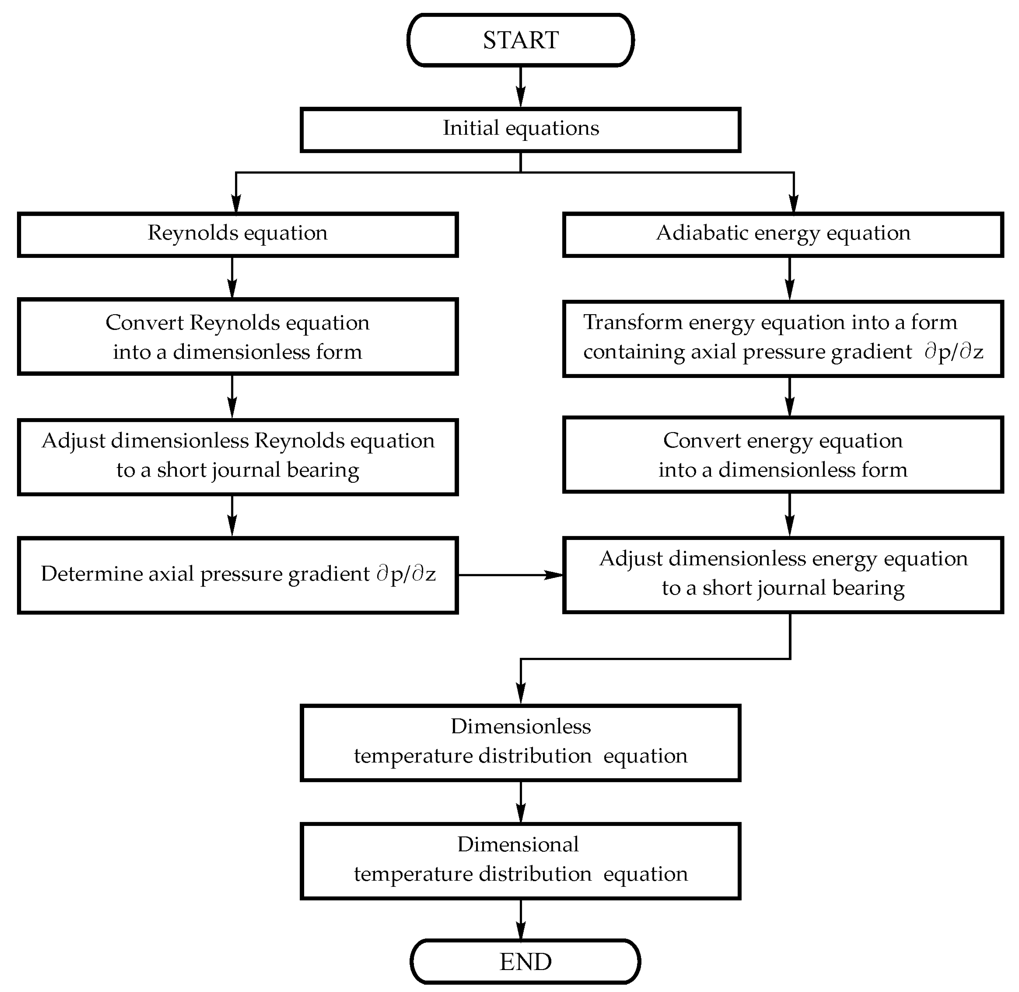
For a better understanding of the entire work, a block diagram of the solution algorithm is given in Figure 2.

Figure 2. The block diagram of the solution algorithm.

3. Solution Procedure

Since the circumferential pressure gradient is neglected in short bearings, the Reynolds and the energy equations have the following form

$$\frac{1}{{\lambda }^2}\frac{\partial }{\partial z{}^{\ast }}\left({\left(h{}^{\ast }\right)}^3\frac{\partial p{}^{\ast }}{\partial z{}^{\ast }}\right)=\frac{dh{}^{\ast }}{d\theta },$$

(7)

$$\frac{\partial T{}^{\ast }}{\partial \theta }-\frac{{\left(h{}^{\ast }\right)}^2}{\lambda {}^2}\frac{\partial p{}^{\ast }}{\partial z{}^{\ast }}\frac{\partial T{}^{\ast }}{\partial z{}^{\ast }}=2\frac{{\left(R/c\right)}^2}{{\left(h{}^{\ast }\right)}^2}+6{\left(R/c\right)}^2{\left(h{}^{\ast }\right)}^2\frac{1}{\lambda {}^2}{\left(\frac{\partial p{}^{\ast }}{\partial z{}^{\ast }}\right)}^2.$$

(8)

By solving the Equation (7), the expression for the axial pressure gradient is obtained

$$\frac{\partial p{}^{\ast }}{\partial z{}^{\ast }}=\frac{dh{}^{\ast }}{d\theta }\frac{{\lambda }^2}{{\left(h{}^{\ast }\right)}^3}\cdot z{}^{\ast }.$$

(9)

Introducing the Equation (9) into the Equation (8) it becomes

$$\frac{\partial T{}^{\ast }}{\partial \theta }-\frac{{\left(h{}^{\ast }\right)}^2}{\lambda {}^2}\frac{dh{}^{\ast }}{d\theta }\frac{{\lambda }^2}{{\left(h{}^{\ast }\right)}^3}\cdot z{}^{\ast }\cdot \frac{\partial T{}^{\ast }}{\partial z{}^{\ast }}=2\frac{{\left(R/c\right)}^2}{{\left(h{}^{\ast }\right)}^2}+6{\left(R/c\right)}^2{\left(h{}^{\ast }\right)}^2\frac{1}{\lambda {}^2}{\left(\frac{dh{}^{\ast }}{d\theta }\frac{{\lambda }^2}{{\left(h{}^{\ast }\right)}^3}z{}^{\ast }\right)}^2$$

(10)

or

$$\frac{\partial T{}^{\ast }}{\partial \theta }-\frac{dh{}^{\ast }}{d\theta }\frac{1}{h{}^{\ast }}\cdot z{}^{\ast }\cdot \frac{\partial T{}^{\ast }}{\partial z{}^{\ast }}=2\frac{{\left(R/c\right)}^2}{{\left(h{}^{\ast }\right)}^2}+6{\lambda }^2{\left(R/c\right)}^2{\left(\frac{dh{}^{\ast }}{d\theta }\right)}^2\frac{{\left(z{}^{\ast }\right)}^2}{{\left(h{}^{\ast }\right)}^4}.$$

(11)

The solution of the Equation (11) is assumed in the form

$$T{}^{\ast }\left(\theta ,z{}^{\ast }\right)=f\left(\theta \right)\cdot {\left(z{}^{\ast }\right)}^2+g\left(\theta \right),$$

(12)

where $f\left(\theta \right)$ and $g\left(\theta \right)$ are the functions to be determined.

Finding partial derivatives of the Equation (12) for $\theta$ and $z{}^{\ast }$

$$\frac{\partial T{}^{\ast }}{\partial \theta }=f^{\prime }\left(\theta \right)\cdot {\left(z{}^{\ast }\right)}^2+g^{\prime }\left(\theta \right),$$

(13)

$$\frac{\partial T{}^{\ast }}{\partial z{}^{\ast }}=2f\left(\theta \right)\cdot z{}^{\ast },$$

(14)

and substituting them into the Equation (11) it gives

$$f^{\prime }\left(\theta \right)\cdot {\left(z{}^{\ast }\right)}^2+g^{\prime }\left(\theta \right)+2\frac{\epsilon \sin \theta }{\left(1+\epsilon \cos \theta \right)}f\left(\theta \right)\cdot {\left(z{}^{\ast }\right)}^2=\frac{2{\left(R/c\right)}^2}{{\left(1+\epsilon \cos \theta \right)}^2}+6{\lambda }^2\frac{{\left(R/c\right)}^2\epsilon {}^2{\sin }^2\theta }{{\left(1+\epsilon \cos \theta \right)}^4}\cdot {\left(z{}^{\ast }\right)}^2.$$

(15)

By grouping the terms containing ${\left(z{}^{\ast }\right)}^2$ and the terms that are functions only of $\theta$ into two separate groups, the following equations are obtained

$$f^{\prime }\left(\theta \right)\cdot {\left(z{}^{\ast }\right)}^2+2\frac{\epsilon \sin \theta }{\left(1+\epsilon \cos \theta \right)}f\left(\theta \right)\cdot {\left(z{}^{\ast }\right)}^2=6{\lambda }^2\frac{{\left(R/c\right)}^2\epsilon {}^2{\sin }^2\theta }{{\left(1+\epsilon \cos \theta \right)}^4}\cdot {\left(z{}^{\ast }\right)}^2,$$

(16)

$$g^{\prime }\left(\theta \right)=\frac{2{\left(R/c\right)}^2}{{\left(1+\epsilon \cos \theta \right)}^2}.$$

(17)

After dividing the Equation (16) with ${\left(z{}^{\ast }\right)}^2$, we get

$$f^{\prime }\left(\theta \right)+2\frac{\epsilon \sin \theta }{\left(1+\epsilon \cos \theta \right)}f\left(\theta \right)=6{\lambda }^2\frac{{\left(R/c\right)}^2\epsilon {}^2{\sin }^2\theta }{{\left(1+\epsilon \cos \theta \right)}^4}.$$

(18)

The Equation (18) is a linear, non-homogeneous equation, solved by the constant variation method. For this purpose, only the homogeneous part of the differential equation is observed and it has the form

$$f^{\prime }\left(\theta \right)+2\frac{\epsilon \sin \theta }{\left(1+\epsilon \cos \theta \right)}f\left(\theta \right)=0.$$

(19)

The newly obtained homogeneous differential equation is separable, i.e.,

$$\frac{df}{f}=-2\frac{\epsilon \sin \theta }{\left(1+\epsilon \cos \theta \right)}d\theta .$$

(20)

After introducing the substitution

$$u=1+\epsilon \cos \theta ,$$

(21)

the Equation (20) becomes

$$\frac{df}{f}=2\frac{du}{u}.$$

(22)

Integrating the Equation (22) gives

$$\ln (f)=\ln \left(C\cdot u^2\right),$$

(23)

i.e.,

$$f=C\cdot {(1+\epsilon \cos \theta )}^2,$$

(24)

where $C$ is an integration constant for the homogeneous differential equation. As the non-homogeneous differential equation is solved here, then $C$ is actually a function of $\theta$. In order to determine $C(\theta )$, the Equation (24) should be introduced into the Equation (18), which gives a new differential equation

$$\begin{array}{c}\frac{dC}{d\theta }\cdot {(1+\epsilon \cos \theta )}^2-2C\cdot (1+\epsilon \cos \theta )\cdot \epsilon \sin \theta +2\frac{\epsilon \sin \theta }{\left(1+\epsilon \cos \theta \right)}\cdot C\cdot {(1+\epsilon \cos \theta )}^2=\\ =6{\lambda }^2\frac{{\left(R/c\right)}^2\epsilon {}^2{\sin }^2\theta }{{\left(1+\epsilon \cos \theta \right)}^4}.\end{array}$$

(25)

i.e.,

$$\frac{dC}{d\theta }\cdot {(1+\epsilon \cos \theta )}^2=6{\lambda }^2\frac{{\left(R/c\right)}^2\epsilon {}^2{\sin }^2\theta }{{\left(1+\epsilon \cos \theta \right)}^4}$$

(26)

or

$$dC=6{\lambda }^2\frac{{\left(R/c\right)}^2\epsilon {}^2{\sin }^2\theta }{{\left(1+\epsilon \cos \theta \right)}^6}d\theta .$$

(27)

The solution of the Equation (27) may be written in the general form

$$C\left(\theta \right)=6{\left(R/c\right)}^2{\lambda }^2\epsilon {}^2\cdot I_6^{20},$$

(28)

where

$$I_6^{20}={\displaystyle \int \frac{{\left(\sin \theta \right)}^2}{{\left(1+\epsilon \cos \theta \right)}^6}d\theta }.$$

(29)

The integral from the Equation (29) is of the type

$$I_n^{lm}={\displaystyle \int \frac{{\sin }^l\theta \cdot {\cos }^m\theta }{{\left(1+\epsilon \cos \theta \right)}^n}}d\theta ,$$

(30)

and its solving is shown in Appendix B. The solution is

$$\begin{array}{c}{I}_6^{20}=\left(1-{\epsilon }^2\right){}^{-9/2}\cdot \left(\frac{1}{2}+\frac{3}{8}{\epsilon }^2\right)\cdot \arccos \left(\frac{\epsilon +\cos \theta }{1+\epsilon \cos \theta }\right)-\epsilon \left(1-{\epsilon }^2\right){}^{-4}\cdot \left(\frac{3}{4}+\frac{1}{8}{\epsilon }^2\right)\cdot \frac{\sin \theta }{1+\epsilon \cos \theta }-\\ -\frac{1}{2}{\left(1-{\epsilon }^2\right)}^{-4}\cdot \frac{\sin \theta \cdot \left(\epsilon +\cos \theta \right)}{{\left(1+\epsilon \cos \theta \right)}^2}+\epsilon {\left(1-{\epsilon }^2\right)}^{-4}\cdot \left(\frac{3}{4}+\frac{1}{16}{\epsilon }^2\right)\cdot \frac{\sin \theta \cdot {\left(\epsilon +\cos \theta \right)}^2}{{\left(1+\epsilon \cos \theta \right)}^3}-\\ -\epsilon {\left(1-{\epsilon }^2\right)}^{-3}\cdot \left(\frac{1}{4}+\frac{1}{48}{\epsilon }^2\right)\cdot \frac{{\sin }^3\theta }{{\left(1+\epsilon \cos \theta \right)}^3}-\\ -\frac{3}{8}{\epsilon }^2\left({\left(1-{\epsilon }^2\right)}^{-4}\frac{\sin \theta \cdot {\left(\epsilon +\cos \theta \right)}^3}{{\left(1+\epsilon \cos \theta \right)}^4}-{\left(1-{\epsilon }^2\right)}^{-3}\cdot \frac{{\sin }^3\theta \cdot \left(\epsilon +\cos \theta \right)}{{\left(1+\epsilon \cos \theta \right)}^4}\right)+\\ +\frac{1}{80}{\epsilon }^3\left(5{\left(1-{\epsilon }^2\right)}^{-4}\frac{\sin \theta \cdot {\left(\epsilon +\cos \theta \right)}^4}{{\left(1+\epsilon \cos \theta \right)}^5}-10{\left(1-{\epsilon }^2\right)}^{-3}\cdot \frac{{\sin }^3\theta \cdot {\left(\epsilon +\cos \theta \right)}^2}{{\left(1+\epsilon \cos \theta \right)}^5}\right)+\\ +\frac{1}{80}{\epsilon }^3\left({\left(1-{\epsilon }^2\right)}^{-2}\cdot \frac{{\sin }^5\theta }{{\left(1+\epsilon \cos \theta \right)}^5}\right)+{D^{\prime }}_2.\end{array}$$

(31)

After substituting the Equation (31) in the Equation (28), it can be written

$$C\left(\theta \right)=6{\left(R/c\right)}^2{\lambda }^2\epsilon {}^2\cdot I_6^{20}+D_2,$$

(32)

where $D_2$ is a new integration constant.

The Equation (24) now becomes

$$f\left(\theta \right)=\left(6{\left(R/c\right)}^2{\lambda }^2\epsilon {}^2\cdot I_6^{20}+D_2\right)\cdot {(1+\epsilon \cos \theta )}^2.$$

(33)

After determining the function $f(\theta )$, the function $g(\theta )$ is determined by solving the Equation (17). With respect to the Equation (30), the function $g(\theta )$ may be written in the form

$$g\left(\theta \right)=2{\left(R/c\right)}^2\cdot I_2^{00}.$$

(34)

The solving of integral $I_2^{00}$ is described in Appendix B and the solution is

$$I_2^{00}=\frac{1}{{\left(1-{\epsilon }^2\right)}^{3/2}}\cdot \left(\arccos \left(\frac{\epsilon +\cos \theta }{1+\epsilon \cos \theta }\right)-\epsilon \cdot {\left(1-{\epsilon }^2\right)}^{1/2}\cdot \frac{\sin \theta }{1+\epsilon \cos \theta }\right)+{D^{\prime }}_3.$$

(35)

Now it is

$$g\left(\theta \right)=\frac{2{\left(R/c\right)}^2}{\left(1-{\epsilon }^2\right)}\left[\frac{1}{{\left(1-{\epsilon }^2\right)}^{1/2}}\arccos \left(\frac{\epsilon +\cos \theta }{1+\epsilon \cos \theta }\right)-\frac{\epsilon \sin \theta }{\left(1+\epsilon \cos \theta \right)}\right]+D_3,$$

(36)

where $D_3$ is a new integration constant.

Taking into account the Equations (33) and (36), the Equation (12) becomes

$$\begin{array}{c}T{}^{\ast }\left(\theta ,z{}^{\ast }\right)=\left[6{\left(\frac{R}{c}\right)}^2{\lambda }^2\epsilon {}^2\cdot I_6^{20}+D_2\right]\cdot {(1+\epsilon \cos \theta )}^2{\left(z{}^{\ast }\right)}^2+\\ +2{\left(\frac{R}{c}\right)}^2\frac{1}{\left(1-{\epsilon }^2\right)}\left[\frac{1}{{\left(1-{\epsilon }^2\right)}^{1/2}}\arccos \left(\frac{\epsilon +\cos \theta }{1+\epsilon \cos \theta }\right)-\frac{\epsilon \sin \theta }{\left(1+\epsilon \cos \theta \right)}\right]+D_3.\end{array}$$

(37)

The constants $D_2$ and $D_3$ are determined from the boundary condition $T{}^{\ast }\left(0,z{}^{\ast }\right)=T_0{}^{\ast }$, where $T_0{}^{\ast }$ is the dimensionless temperature of the oil at $\theta =0$. The boundary condition is based on the assumption that the oil temperature does not change in the area between the oil inlet (vertical plane) and the attitude plane defined by the angle $\Phi$ (Figure 1). Hence, Equation (37) becomes

$$T{}^{\ast }\left(0,z{}^{\ast }\right)=D_2\cdot {(1+\epsilon )}^2{\left(z{}^{\ast }\right)}^2+D_3=T_0{}^{\ast }.$$

(38)

Also, it is assumed that the temperature $T_0{}^{\ast }$ is constant along the axis of the bearing. In other words, it is independent of the coordinate $z{}^{\ast }$, so it must be $D_2=0$. Therefore, $D_3=T_0{}^{\ast }$ and the Equation (38) becomes

$$\begin{array}{c}T{}^{\ast }\left(\theta ,z{}^{\ast }\right)=6{\left(\frac{R}{c}\right)}^2{\lambda }^2\epsilon {}^2\cdot I_6^{20}\cdot {(1+\epsilon \cos \theta )}^2{\left(z{}^{\ast }\right)}^2+\\ +2{\left(\frac{R}{c}\right)}^2\frac{1}{\left(1-{\epsilon }^2\right)}\left[\frac{1}{{\left(1-{\epsilon }^2\right)}^{1/2}}\arccos \left(\frac{\epsilon +\cos \theta }{1+\epsilon \cos \theta }\right)-\frac{\epsilon \sin \theta }{\left(1+\epsilon \cos \theta \right)}\right]+T_0{}^{\ast }.\end{array}$$

(39)

By using the expression for the dimensionless temperature from the Equation (4), the Equation (39) can be transformed into the form

$$\begin{array}{c}T\left(\theta ,z{}^{\ast }\right)\cdot \frac{\rho c_p}{\eta \omega }=6{\left(\frac{R}{c}\right)}^2{\lambda }^2\epsilon {}^2\cdot I_6^{20}\cdot {(1+\epsilon \cos \theta )}^2{\left(z{}^{\ast }\right)}^2+\\ +2{\left(\frac{R}{c}\right)}^2\frac{1}{\left(1-{\epsilon }^2\right)}\left[\frac{1}{{\left(1-{\epsilon }^2\right)}^{1/2}}\arccos \left(\frac{\epsilon +\cos \theta }{1+\epsilon \cos \theta }\right)-\frac{\epsilon \sin \theta }{\left(1+\epsilon \cos \theta \right)}\right]+T_0\cdot \frac{\rho c_p}{\eta \omega },\end{array}$$

(40)

i.e.,

$$\begin{array}{c}T\left(\theta ,z{}^{\ast }\right)=6\frac{\eta \omega }{\rho c_p}\cdot {\left(\frac{R}{c}\right)}^2{\lambda }^2\epsilon {}^2\cdot I_6^{20}\cdot {(1+\epsilon \cos \theta )}^2{\left(z{}^{\ast }\right)}^2+\\ +2\frac{\eta \omega }{\rho c_p}{\left(\frac{R}{c}\right)}^2\frac{1}{\left(1-{\epsilon }^2\right)}\left[\frac{1}{{\left(1-{\epsilon }^2\right)}^{1/2}}\arccos \left(\frac{\epsilon +\cos \theta }{1+\epsilon \cos \theta }\right)-\frac{\epsilon \sin \theta }{\left(1+\epsilon \cos \theta \right)}\right]+T_0.\end{array}$$

(41)

The Equation (41) is the final analytic form of the temperature distribution in the oil film of short journal bearing.

While deriving this equation, it is assumed that the viscosity of oil is not changed with the temperature, which is also one of the assumptions that the Reynolds equation derivation is based on. This is justified to some extent, since journal bearings are dominantly used in internal combustion engines, where they are lubricated by so-called multi grade oils, characterized by their viscosity resistance to temperature change. On the other hand, by introducing this assumption, a considerably simpler theoretical model of temperature distribution in the oil film is derived, on the basis of which satisfactory results can be obtained quite quickly.

4. Results and Discussion

In order to validate the mathematical model of temperature distribution in a journal bearing oil film (Equation (41)), the experimental results given in the reference [25] were used. In that sense, the bearing parameters were also taken from the reference [25] and are presented in Table 1.

Table 1. Basic parameters of the journal bearing.

Parameter	Unit	Value
$\mathrm{Journal}\mathrm{radius},R$	m	0.05
$\mathrm{Bearing}\mathrm{length},L$	m	0.08
$\mathrm{Clearance}\mathrm{ratio},c/R$	-	0.0029
$\mathrm{Lubricant}\mathrm{viscosity}\mathrm{at}40{}^{\mathrm{o}}\mathrm{C},\eta$	Pa s	0.0277
$\mathrm{Lubricant}\mathrm{density}\mathrm{at}40{}^{\mathrm{o}}\mathrm{C},\rho$	kg/m3	860
$\mathrm{Lubricant}\mathrm{specific}\mathrm{heat},c_p$	$\mathrm{J}/(\mathrm{kg}{}^{\mathrm{o}}\mathrm{C})$	2000
$\mathrm{Inlet}\mathrm{lubricant}\mathrm{temperature},T_0$	${}^{\mathrm{o}}\mathrm{C}$	40
$\mathrm{Journal}\mathrm{speed}\left(\mathrm{lower}\mathrm{value}\right),n$	rpm	2000
$\mathrm{Journal}\mathrm{speed}\left(\mathrm{higher}\mathrm{value}\right),n$	rpm	4000
$\mathrm{Bearing}\mathrm{load}\left(\mathrm{lower}\mathrm{value}\right),F$	N	4000
$\mathrm{Bearing}\mathrm{load}\left(\mathrm{higher}\mathrm{value}\right),F$	N	6000

The operating point of the bearing is defined by the force $F$ and journal speed $n$ and the two parameters significantly affect the eccentricity ratio $\epsilon$. In order to apply the temperature distribution Equation (41) to the data in Table 1, it is necessary to relate the parameters $F$, $n$ and $\epsilon$ to each other. The parameters are related by the equation of the load capacity that is given in the form [8]

$$F=\frac{\eta \cdot \omega \cdot R\cdot L^3}{4\cdot c^2}\cdot \frac{\epsilon }{{(1-{\epsilon }^2)}^2}\cdot {\left(16\cdot {\epsilon }^2+{\pi }^2\cdot (1-{\epsilon }^2)\right)}^{1/2}.$$

(42)

By introducing the data from Table 1 into the Equation (42) and applying the “trial and error” method to the Equation (42) it is found that the value $\epsilon =0.44$ corresponds to the operating point ($F=4000\mathrm{N}$, $n=2000\mathrm{rpm}$), and the value $\epsilon =0.38$ corresponds to the operating point ($F=6000\mathrm{N}$, $n=4000\mathrm{rpm}$). The corresponding values of attitude angle $\Phi$ are 58.04° and 62.39°, respectively. Furthermore, by substituting the data from Table 1 and the corresponding $\epsilon$ values into the Equation (41), the theoretical oil film temperature distribution in the midplane cross-section of the bearing has been obtained at the two operating points.

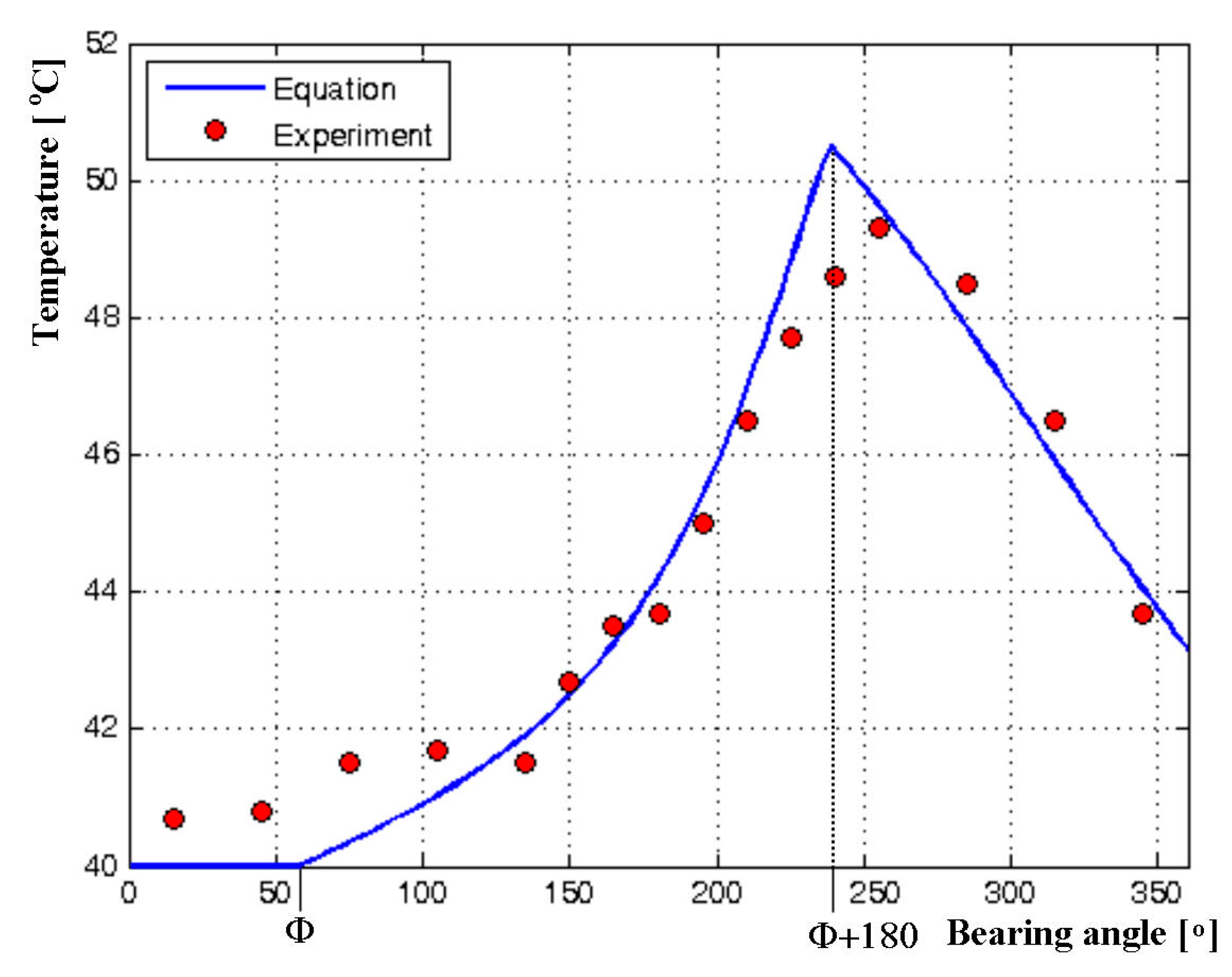
The first operating point is defined by the journal speed of $n$ = 2000 rpm and the load of $F$ = 4000 N. The theoretical temperature distribution corresponding to that operating point is represented by the blue line in Figure 3. In Figure 3, the oil temperature values measured under the same operation conditions are also plotted and marked by the red circles. Similarly, Figure 4 shows the theoretical temperature distribution and the corresponding experimental values [25], at $n$ = 4000 rpm and $F$ = 6000 N.

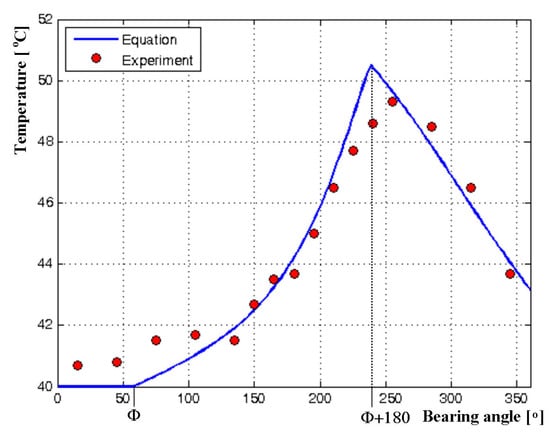
Figure 3. Oil film temperature distribution at $n$ = 2000 rpm and $F$ = 4000 N.

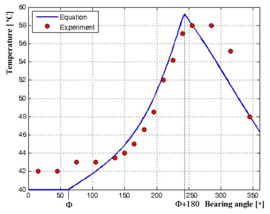
Figure 4. Oil film temperature distribution at $n$ = 4000 rpm and $F$ = 6000 N.

Looking at the both diagrams, one can notice that in the area where the bearing angle is less than $\Phi$, the measured oil temperature is slightly higher than at the oil inlet. That is the result of mixing the oil that enters the bearing with the oil that is already inside the bearing. This phenomenon is not taken into account while deriving the temperature distribution equation, hence the deviation of about 1–2 °C in relation to the previous assumption about the temperature constancy in the bearing area between the oil supply and the attitude plane. However, this assumption is justified by the fact that the experimental data show a slight change in temperature in the mentioned area.

In the area of temperature rise (the area between the angle $\Phi$ and $\Phi$ + 180), there is a very good agreement between the experimental and theoretical values with a deviation of up to 2 °C, at both operating points considered. Furthermore, the maximum oil temperature calculated is slightly higher than the maximum temperature measured, which can be useful if one wants to predict critical operating points of the bearing.

In the area between the bearing angle corresponding to the maximum temperature and the bearing angle corresponding to the oil inlet, temperature decreases. A fairly good agreement between theoretical and experimental results is clearly seen when the bearing operates under light-duty conditions (Figure 3). However, for heavier operating conditions (Figure 4), the deviation is slightly higher (up to about 3 °C).

A more complete view of temperature distribution in the oil film of the bearing is enabled by a 3D-diagram showing the temperature change along both the bearing circumference and length. Such a diagram for the bearing considered at $n$ = 4000 rpm and $F$ = 6000 N, is shown in Figure 5. It is noted that the temperature variation along the axis of the bearing has a slightly parabolic shape that is symmetrical in relation to the bearing midplane ($z{}^{\ast }=0$). Furthermore, the temperature decreases from the side planes to the midplane of the bearing. A similar temperature distribution was obtained experimentally by Mitsui et al. [26].

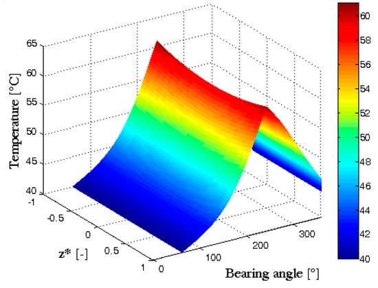
Figure 5. 3D temperature distribution in the bearing oil film, at $n$ = 4000 rpm and $F$ = 6000 N.

The good agreement of the derived equation with the experimental data is encouraging when it comes to the possibility of its application. The authors hope that such an equation could serve to estimate the temperature of the oil film quickly, which may be useful in a diagnostic tool designed to monitor the bearing conditions in real time. A detailed analysis of the possibility of applying the derived equation in a diagnostic tool, as well as its potential implementation, could be a topic for future research. In the text to follow, only a hint is given of how this equation could work in real time.

Most of the input data in Equation (41) are constants, while the others depend on operating parameters of the bearing. The constants are:

—

characteristics of the oil used (density $\rho$, viscosity $\eta$ and specific heat at constant pressure $c_p$) and

—

geometric parameters of the bearing (bearing radius $R$, radial clearance $c$ and bearing length $L$).

These constants do not affect the real time monitoring concept and their values are stored in the computer’s memory.

On the other hand, the operating parameters (oil inlet temperature $T_0$, journal speed $n$ and bearing load $F$) are measured using appropriate sensors. On the basis of the measured values, the angular velocity $\omega$ and eccentricity ratio $\epsilon$ are calculated.

Such a scenario could be possible for steady-state conditions of the bearing operation. After each transition from one steady-state condition to another, the temperature distribution should be recalculated.

5. Conclusions

In this paper, the equation of temperature field in the oil film of short journal bearing is derived analytically. The results of applying this equation to a journal bearing have been compared to the corresponding experimental results of other researchers for the same bearing, showing a small deviation. The good agreement of the derived equation with experimental data, as well as its explicit analytical form, allows for temperature distribution in the oil film to be determined quickly, with satisfactory accuracy but without demanding computer resources. This indicates that the derived equation might be useful in a computer diagnostic tool as a part of a more complex procedure for the real time monitoring of the bearing condition.

Another contribution of this research is that the energy equation is transformed into a form, which allows it to be coupled with the Reynolds equation for short journal bearing. As a result, a partial differential equation of the temperature field for a short bearing is obtained, which is in the form that allows it to be solved analytically and, as far as the authors are aware, it is not encountered in any previous literature.

References

- Pinkus, O. The Reynolds Centennial: A Brief History of the Theory of Hydrodynamic Lubrication. Trans. ASME J. Tribol. 1987, 109, 2–15. [Google Scholar] [CrossRef]
- Brito, F.P. Thermohydrodynamic Performance of Twin Groove Journal Bearings Considering Realistic Lubricant Supply Conditions: A Theoretical and Experimental Study. PhD Thesis, University of Minho, Braga, Portugal, 2009. [Google Scholar]
- Stachowiak, G.W.; Batchelor, A.W. Engineering Tribology, 3rd ed.; Elsevier Butterworth-Heinemann: Amsterdam, The Netherlands; Boston, MA, USA, 2005. [Google Scholar]
- Colynuck, A.J.; Medley, J.B. Comparison of Two Finite Difference Methods for the Numerical Analysis of Thermohydrodynamic Lubrication. Tribol. Trans. 1989, 32, 346–356. [Google Scholar] [CrossRef]
- Pinkus, O. Thermal Aspects of Fluid Film Tribology; ASME Press: New York, NY, USA, 1990. [Google Scholar]
- Harnoy, A. Bearing Design in Machinery—Engineering Tribology and Lubrication; Mechanical Engineering; Marcel Dekker: New York, NY, USA, 2003. [Google Scholar]
- Szeri, A.Z. Fluid Film Lubrication: Theory and Design; Cambridge University Press: Cambridge, UK, 1998. [Google Scholar]
- Frene, J.; Nicolas, D.; Degueurce, B.; Berthe, D.; Godet, M. Hydrodynamic Lubrication: Bearings and Thrust Bearings; Elsevier: Burlington, MA, USA, 1997. [Google Scholar]
- Cameron, A. Basic Lubrication Theory, 2d ed.; Horwood, E., Ed.; Halsted Press: Chichester, UK; New York, NY, USA, 1976. [Google Scholar]
- Cope, W.F. The hydrodynamical theory of film lubrication. Proc. R. Soc. Lond. Ser. Math. Phys. Sci. 1949, 197, 201–217. [Google Scholar] [CrossRef]
- Stokes, M.J.; Ettles, C.M.M. A General Evaluation Method for the Diabatic Journal Bearing. Proc. R. Soc. Math. Phys. Eng. Sci. 1974, 336, 307–325. [Google Scholar] [CrossRef]
- Fillon, M.; Bouyer, J. Thermohydrodynamic analysis of a worn plain journal bearing. Tribol. Int. 2004, 37, 129–136. [Google Scholar] [CrossRef]
- Sehgal, R.; Swamy, K.N.S.; Athre, K.; Biswas, S. A comparative study of the thermal behaviour of circular and non-circular journal bearings. Lubr. Sci. 2000, 12, 329–344. [Google Scholar] [CrossRef]
- Banwait, S.S.; Chandrawat, H.N. Study of thermal boundary conditions for a plain journal bearing. Tribol. Int. 1998, 31, 289–296. [Google Scholar] [CrossRef]
- Mishra, P.C.; Pandey, R.K.; Athre, K. Temperature profile of an elliptic bore journal bearing. Tribol. Int. 2007, 40, 453–458. [Google Scholar] [CrossRef]
- Moreno Nicolás, J.A.; Gómez de León Hijes, F.C.; Alhama, F. Solution of temperature fields in hydrodynamics bearings by the numerical network method. Tribol. Int. 2007, 40, 139–145. [Google Scholar] [CrossRef]
- Pierre, I.; Electricite de France; Bouyer, J.; Fillon, M. Thermohydrodynamic Behavior of Misaligned Plain Journal Bearings: Theoretical and Experimental Approaches. Tribol. Trans. 2004, 47, 594–604. [Google Scholar] [CrossRef]
- Chauhan, A.; Sehgal, R.; Sharma, R.K. Thermohydrodynamic analysis of elliptical journal bearing with different grade oils. Tribol. Int. 2010, 43, 1970–1977. [Google Scholar] [CrossRef]
- Durany, J.; Pereira, J.; Varas, F. Numerical solution to steady and transient problems in thermohydrodynamic lubrication using a combination of finite element, finite volume and boundary element methods. Finite Elem. Anal. Des. 2008, 44, 686–695. [Google Scholar] [CrossRef]
- Kornaev, A.V.; Kornaeva, E.P.; Savin, L.A. Theoretical Premises of Thermal Wedge Effect in Fluid-Film Bearings Supplied with a Nonhomogeneous Lubricant. Int. J. Mech. 2017, 11, 197–203. [Google Scholar]
- Babin, A.; Kornaev, A.; Rodichev, A.; Savin, L. Active thrust fluid-film bearings: Theoretical and experimental studies. Proc. Inst. Mech. Eng. Part J J. Eng. Tribol. 2020, 234, 261–273. [Google Scholar] [CrossRef]
- Li, S.; Ao, H.; Jiang, H.; Korneev, A.Y.; Savin, L.A. Steady characteristics of the water-lubricated conical bearings. J. Donghua Univ. Engl. Ed. 2012, 29, 115–122. [Google Scholar]
- Norton, R.L. Machine Design: An Integrated Approach, 4th ed.; Prentice Hall: Boston, MA, USA, 2011. [Google Scholar]
- Khonsari, M.M.; Booser, E.R. Applied Tribology: Bearing Design and Lubrication, 3rd ed.; John Wiley & Sons Inc.: Hoboken, NJ, USA, 2017. [Google Scholar]
- Ferron, J.; Frene, J.; Boncompain, R. A Study of the Thermohydrodynamic Performance of a Plain Journal Bearing Comparison between Theory and Experiments. Trans. ASME J. Lubr. Technol. 1983, 105, 422–428. [Google Scholar] [CrossRef]
- Mitsui, J.; Hori, Y.; Tanaka, M. An Experimental Investigation on the Temperature Distribution in Circular Journal Bearings. Trans. ASME J. Tribol. 1986, 108, 621–626. [Google Scholar] [CrossRef]
© 2020 by the authors. Licensee MDPI, Basel, Switzerland. This article is an open access article distributed under the terms and conditions of the Creative Commons Attribution (CC BY) license (http://creativecommons.org/licenses/by/4.0/).