Comparison of Three Availability Systems with Warm Standby Components, Detection Delay, and General Repair Times

Abstract

This study analyzes three availability systems with warm standby units, fault detection delay, and general repair times. The failure times and repair times of failed components were assumed to follow exponential and general distributions, respectively. The detection delay times were assumed to be exponentially distributed. This study exploited the supplementary variable technique to develop a recursive method for deriving the steady-state availability for three systems. By using extensive numerical computations, we compared three systems in terms of system availability based on specific values given to the system parameters. The state transition rate diagrams of the three systems revealed the symmetry property approximately. The three systems were ranked based on the system availability and the cost/benefit for the three various repair time distributions: exponential, three-stage Erlang, and deterministic, where the benefit was system availability.

1. Introduction

System availability plays an increasingly important role in many real-world systems, such as manufacturing systems, computer systems, and power plants. To preserve a high or given level of system availability that is often necessary for these practical systems, standby components are usually used to increase system availability. There are two kinds of standby components. A cold standby component never fails, whereas a warm standby component can fail, where its failure rate is higher than zero but less than that of a primary component. On the other hand, when a primary or standby component fails, many real systems (for example, see Trivedi [1]) require a detection delay period to detect the fault before it can be repaired. Furthermore, the system is assumed to be in a down state during the detection delay (Trivedi [1]). This study proposes a form of steady-state availability analysis of repairable systems with warm standby components, a detection delay, and general repair times. The relevant literature is outlined below.

The supplementary variable was first proposed by Cox [2] to transform a non-Markovian model into a Markovian one. Since then, many studies exploited this technique to analyze different non-Markovian systems in the queueing literature. Hokstad [3] utilized the supplementary variable technique to analyze the M/G/1 queue in 1975. Based on this technique, Gupta and Rao [4] and Gupta and Rao [5] proposed a recursive method to derive the steady-state probability of the M/G/1 machine repair problem without standbys and the M/G/1 machine repair problem with cold standbys, respectively. This technique was applied to analyze the G/M/1 queueing system with an N-policy and finite capacity by Ke and Wang [6]. Zhang and Wu [7] used the supplementary variable technique to propose a method for the reliability analysis of a machine repair system with k out n spare units and an F-policy. Shakuntla et al. [8] exploited this technique to propose reliability analysis for the polytube industry. This technique was utilized to analyze an M/G/1 machine repair system under multiple imperfect coverages by Wang et al. [9]. According to the supplementary variable technique, Ke et al. [10] proposed a method for analyzing the machine repair problem with a working breakdown repairman and standbys having an imperfect switchover.

In the literature regarding the analysis of repairable systems, several studies have addressed the comparison of various systems. Wang and Pearn [11] studied the cost–benefit analysis of series systems with warm standbys. They derived explicit expressions for the mean time to first system failure and system availability for three systems. Wang and Chiu [12] presented the cost–benefit analysis of queueing systems with warm standby components and imperfect coverage. Furthermore, they explored a comparative analysis associated with numerical results to verify the effects of parameters on the cost/benefit ratios. Wang and Chen [13] discussed system availability among three systems with a reboot delay, switching failures, and general repair times. Singh et al. [14] evaluated the transitional state probabilities, system reliability, system availability, mean time to first system failure, and the cost of the system by using the supplementary variable technique. Yu et al. [15] proposed a method to optimize the availability of a system where the objective of their study was to minimize the system cost under the constraint that system availability must maintain a given level.

The concept of a detection delay for a repairable system was introduced by Trivedi [13]. Ke et al. [16] analyzed a machine repair system with detection, imperfect coverage, and reboot using a Bayesian approach. Kleyner and Volovoi [17] proposed an application of stochastic Petri nets to calculate the availability of systems where partial detection was considered. Ke and Liu [18] studied a machine repair system with imperfect coverage and reboot. They derived the steady-state probabilities for the number of down units during an arbitrary period. Moreover, they presented the sensitivity analysis of the steady-state availability with respect to the system parameters for different repair time distributions.

The problem studied in this paper is more general than the work of Trivedi [1]. To our knowledge, the explicit expression for the availability of a system with a detection delay and the repair time has a general distribution has not been derived. The purpose of this study was to accomplish three objectives. The first was to derive the steady-state availability for three systems by exploiting the supplementary variables treated as the remaining repair times. The explicit expressions for the steady-state availability for three different repair time distributions: exponential (M), k-stage Erlang $({\mathrm{E}}_k)$, and deterministic (D) were obtained. The second was to perform a numerical analysis in terms of $Av$ and cost/Av for three different repair time distributions. The third was to rank three systems for the $Av$ and cost/Av based on specific values of system parameters and the unit costs of the components.

The rest of this paper is organized as follows. Three availability systems are described in Section 2. A practical application of this model is also provided in this section. Notations used in this study are defined in Section 3. Section 4 derives the availability of each of the three availability systems based on the supplementary variable technique. Extensive numerical examples are provided and executed to compare the three systems when both Av and cost/Av are considered in Section 5. Finally, Section 6 presents a summary and conclusions.

2. Description of the Three Availability Systems

This study assumed that a data center requires 30 MW of electrical power and that the power of the components is available in units of 30 MW, 15 MW, and 10 MW. To maintain reliable and stable system availability, there were warm standby components, and all primary and warm standby components were continuously monitored using a fault-detecting device to identify whether they fail. When a primary or warm standby component failed, we assumed that it could be repaired. The times to failure for the primary components and those for the warm standby components had exponential distributions with parameters $\lambda$ and $\alpha$ $(0<\alpha <\lambda <1)$, respectively, and these failure times were independent of each other. When one primary component failed, a warm standby component (if one is available), with a failure rate $\alpha$, is immediately converted into a primary one with a failure rate $\lambda$. Whenever one component failed, it immediately induced a detection delay. We assumed that the detection delay had an exponential distribution with parameter $\delta$. When the fault was being detected and the last primary component failed, this study assumed that the system failed. Such a fault is called a near-coincident fault. The system was considered to have failed when the standby components were all emptied, which we defined as the state of system failure (sf). It was assumed that the time taken to repair of all failed components were independent of each other and were identically distributed random variables with a distribution function $B(u)(u\ge 0)$, a density function $b(u)(u\ge 0)$, and a mean repair time $b_1$. As long as the electricity generation capacity of the system was less than 30 MW, it would stop working. When a failed component arrived at the repair facility and observed that a server was available, it would be immediately repaired. If a (primary or standby) component failed, it was repaired based on a first-come, first-served (FCFS) basis. We assumed that a server could repair only one failed component at a time and that the service was independent of the failures of the components. Once a failed component was repaired, it was considered as good as new.

This study designed three availability systems as follows: the first system consisted of one 30 MW primary component and one 30 MW warm standby component. The second system consisted of two 15 MW primary components and one 15 MW warm standby component. We assumed that the standby component could replace either one of the initially working components in the case of its failure. The third system was made of three 10 MW primary components and two 10 MW warm standby components. Each standby component could replace either one of the failed working components. If necessary, a standby component could also replace the first used standby component in the case of its failure.

Before analyzing the three availability systems, a practical problem related to the parallel redundant system is presented for illustrative purposes. The virtualization technology plays a pivotal role in the cluster computing environment, especially in adjusting and distributing computing resources. In order to optimize the performance of virtual machines, the system administrator must keep the software packages and OS kernels up to date, especially in the Linux system. We considered a Linux virtual cluster that provided the Linux software mirror service and was managed by the Open Source Cluster Application Resources (OSCAR) cluster management system. The OSCAR head node received requests from the Internet and transmitted them to the client nodes (treated as the primary units). To ensure that every client node was up and running, the ganglia distributed monitoring system was installed to monitor the state of each client node in the virtual cluster. Whenever a failed client node was detected by ganglia, new coming requests were sent to an available client node, and the breakdown client node was terminated. The failed client node was restarted after the error was detected and fixed (failures could be caused by IP conflict, not enough disk space, or operating system fault). The configuration of this Linux virtual cluster is illustrated in Figure 1.

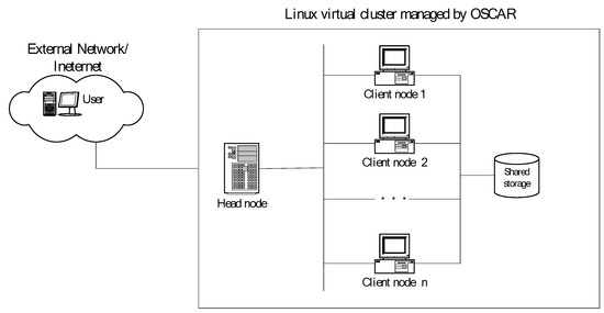
Figure 1. A Linux virtual cluster providing mirror service.

Client nodes are virtual machines and hence can be assumed to be capable of being repaired. Suppose each of the client nodes failed independently of the state of the others and the time-to-failure of each client node was exponentially distributed with a parameter $\lambda$. Whenever one client node fails, OSCAR immediately searches for available client nodes and transmits user requests to them. It was assumed that the detection delay has an exponential distribution with parameter $\delta$. When one client nodes failed, the corresponding virtual machine process was terminated and restarted by the ganglia. Once the client node was restarted, it was considered to be as good as a new one. This study assumed that the times to repair of all failed client nodes were independent to one another with identically distributed random variables with a distribution function $B(u)(u\ge 0)$, a density function $b(u)(u\ge 0)$, and a mean repair time $b_i$.

3. Notations

The following notations and probabilities were defined and used in this study:

$$\lambda \equiv \text{failure rate of a primary component},$$

$$\alpha \equiv \text{failure rate of a warm standby component},$$

$$\delta \equiv \text{detection delay rate},$$

$$B(u)\equiv \text{distribution function} (\mathrm{d}.\mathrm{f}.) \text{of the repair time},$$

$$b(u)\equiv \text{probability density function} (\mathrm{p}.\mathrm{d}.\mathrm{f}.) \text{of the repair time},$$

$$b_1\equiv \text{mean repair time},$$

$$B^{*}(s)\equiv \text{Laplace-Stieltjes transform} (\mathrm{LST}) \text{of} B(u),$$

$$P_{n,m}(t)\equiv \text{probability that exactly} n \text{components are working and} m \text{components are detecting at time} (t\ge 0),$$

$$P_{n,m}^{*}(s)\equiv \text{Laplace–Stieltjes transform} (\mathrm{LST}) \text{of} P_{n,m}(t),$$

$$P_{n,m}^{*(1)}(s)\equiv \text{first order derivative of} P_{n,m}^{*}(s) \text{with respect to} s.$$

4. Availability Analysis

We assumed that the operating system required at least 30 MW power electricity. For each system, the transition rate diagram was drawn, and then the differential equation of each state at time t was derived based on the diagram. Next, we took the Laplace transform on both sides of the differential equation. Finally, the system availability was achieved by working on these Laplace transform equations. In order to manage the general repair times, the following supplementary variable was defined: $U\equiv$ remaining repair time for a given component being repaired. The state of the system at time t is given by:

$$N(t)\equiv \text{number of components that are working in the system},$$

$$M(t)\equiv \text{number of components that are being detected in the system},$$

$$U(t)\equiv \text{remaining repair time for the component being repaired}.$$

The following were also defined:

$$P_{n,m}(u,t)=P\left\{N(t)=n,M(t)=m,u<U(t)\le u+du\right\},u\ge 0,$$

$$P_{n,m}(t)={\displaystyle {\int }_0^{\infty }{P}_{n,m}(u,t)du}.$$

Let $t\to \infty$ such that the following steady-state probabilities can be obtained as follows:

$$P_{n,m}=\underset{t\to \infty }{\lim }{P}_{n,m}(t),$$

and

$$P_{n,m}(u)=\underset{t\to \infty }{\lim }{P}_{n,m}(u,t).$$

4.1. Availability System 1

Availability system 1 included one 30 MW primary component and one 30 MW warm standby component. The state-transition-rate diagram of availability system 1 is shown in Figure 2. Considering the system at time $t$ and $t+dt$ in Figure 2, the following equations of the probability of each state can be derived as follows:

$$\frac{d}{dt}{P}_{2,0}(t)=-(\lambda +\alpha )P_{2,0}(t)+P_{1,0}(0,t),$$

(1)

$$\frac{d}{dt}{P}_{1,1}(t)=-(\lambda +\delta )P_{1,1}(t)+(\lambda +\alpha )P_{2,0}(t),$$

(2)

$$(\frac{\partial }{\partial t}-\frac{\partial }{\partial u})P_{1,0}(u,t)=-\lambda P_{1,0}(u,t)+\delta P_{1,1}(u,t)+b(u)P_{sf}(0,t),$$

(3)

$$(\frac{\partial }{\partial t}-\frac{\partial }{\partial u})P_{sf}(u,t)=\lambda P_{1,0}(u,t)+\lambda P_{1,1}(u,t),$$

(4)

where the state (1,1) denotes the detection stage. The transition from state (1,1) to state (1,0) (at rate ($\delta$) indicates the detection of the fault. The state labeled sf denotes the system failure.

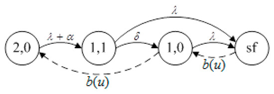
Figure 2. The state transition rate diagram of availability system 1.

We defined:

$$P_{1,1}(u)=b(u)P_{1,1}.$$

(5)

The steady-state equations were obtained from Equations (1)–(4). Next, the Laplace transform was taken on both sides of these equations. By working on the Laplace transform equations, the steady-state availability of availability system 1, $A{v}_1$, can be explicitly derived below:

$$A{v}_1=P_{2,0}+P_{1,0}=\frac{(\lambda +\delta )[\lambda +\alpha -\alpha B^{*}(\lambda )]}{\lambda {\Delta }_1}.$$

(6)

The detailed derivation is provided in Appendix A.

Special Cases

This study investigated three special cases for three different repair time distributions: exponential (M), $k$-stage Erlang $({\mathrm{E}}_k)$, and deterministic (D). The following expressions for the $A{v}_{1M}$, $A{v}_{1E},$ and $A{v}_{1D}$ for three different repair time distributions are shown explicitly below.

Case 1. Exponential repair time

The repair time had an exponential distribution in this case. The mean repair time was set to $b_1=1/\mu$, where $\mu$ was the repair rate. By taking the Laplace transform, we found:

$$B^{*}(\lambda )=\frac{\mu }{\mu +\lambda }.$$

From Equation (6), the expression for the $A{v}_{1M}$ was obtained explicitly as:

$$A{v}_{1M}=\frac{(\lambda +\delta )\left[(\lambda +\alpha )(\mu +\lambda )-\alpha \mu \right]}{\lambda (\mu +\lambda ){\Delta }_1}.$$

Setting $\alpha =\lambda$ in the expression of ${\Delta }_1$, the steady-state probability $P_{2,0}$ for the exponential case is given by:

$$P_{2,0}=\frac{(\lambda +\delta )B^{*}(\lambda )}{{\Delta }_1}=\frac{{\mu }^2(\lambda +\delta )}{{\mu }^2(3\lambda +\delta )+2\lambda [(\lambda +\delta )(\mu +\lambda )+\lambda \mu ]}.$$

From the result of p. 458 of Trivedi [1], the steady-state probability ${\pi }_2$ for exponential case is given by

$${\pi }_2=\frac{{\mu }^2(\lambda +\delta )}{2{\lambda }^2(\lambda +\mu +\delta )E},$$

where

$$E=1+\frac{\mu (\lambda +\delta )}{\lambda (\lambda +\mu +\delta )}+\frac{{\mu }^2}{\lambda (\lambda +\mu +\delta )}+\frac{{\mu }^2(\lambda +\delta )}{2{\lambda }^2(\lambda +\mu +\delta )}.$$

After doing the algebraic manipulation, it is shown that the expression for $P_{2,0}$ is identical to that for ${\pi }_2$.

Case 2. $k$-stage Erlang repair time

The repair time had a $k$-stage Erlang distribution in this case. The $k$-stage Erlang distribution consists of $k$ independent and identical exponential stages, each with a mean $1/(k\mu )$. Taking the Laplace transform, we obtained:

$$B^{*}(\lambda )={\left(\frac{k\mu }{k\mu +\lambda }\right)}^k.$$

From Equation (6) again, the following expression for the $A{v}_{1E}$ was found:

$$A{v}_{1E}=\frac{(\lambda +\delta )\left[(\lambda +\alpha ){(k\mu +\lambda )}^k-\alpha {(k\mu )}^k\right]}{\lambda {(k\mu +\lambda )}^k{\Delta }_1}.$$

Case 3. Deterministic repair time

The repair time distribution was deterministic in this case. In this case, the distribution function of the repair time had the following Laplace transform:

$$B^{*}(\lambda )=e^{\raisebox{1ex}{$-\lambda $}\!\left/ \!\raisebox{-1ex}{$\mu $}\right.}.$$

From Equation (6), the expression for the $A{v}_{1D}$ is derived explicitly to give:

$$A{v}_{1D}=\frac{(\lambda +\delta )(\lambda +\alpha -\alpha e^{\raisebox{1ex}{$-\lambda $}\!\left/ \!\raisebox{-1ex}{$\mu $}\right.})}{\lambda {\Delta }_1}.$$

4.2. Availability System 2

Availability system 2 included two 15 MW primary components and one 15 MW warm standby component. The state-transition-rate diagram of availability system 2 is presented in Figure 3. From Figure 3, the following steady-state equations were derived:

$$0=-\left(2\lambda +\mathsf{\alpha }\right)P_{3,0}+P_{2,0}\left(0\right),$$

(7)

$$0=-(2\lambda +\delta )P_{2,1}+(2\lambda +\alpha )P_{3,0},$$

(8)

$$-\frac{d}{du}{P}_{2,0}(u)=-2\lambda P_{2,0}(u)+\delta b(u)P_{2,1}+b(u)P_{sf}(0),$$

(9)

$$-\frac{d}{du}{P}_{sf}(u)=2\lambda P_{2,0}(u)+2\lambda b(u)P_{2,1},$$

(10)

where we defined:

$$P_{2,1}(u)=b(u)P_{2,1}.$$

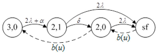
Figure 3. The state transition rate diagram of availability system 2.

We should note that the state labeled (2,1) represents the detection stage. The transition from state (2,1) to state (2,0) indicates the detection of the fault.

A similar argument led to the explicit expression for the steady-state availability of availability system 2, $A{v}_2$, which was given by:

$$A{v}_2=P_{3,0}+P_{2,0}=\frac{(2\lambda +\delta )[2\lambda +\alpha -\alpha B^{*}(2\lambda )]}{2\lambda {\Delta }_2}.$$

(11)

The detailed derivation of $A{v}_2$ is provided in Appendix B.

Special Cases

For availability system 2, three cases for three different repair time distributions: exponential, $k$-stage Erlang, and deterministic are presented. The expressions for the $A{v}_{2M}$, $A{v}_{2E},$ and $A{v}_{2D}$ for three different repair time distributions are listed explicitly as follows:

$$A{v}_{2M}=\frac{(2\lambda +\delta )\left[(2\lambda +\alpha )(\mu +2\lambda )-\alpha \mu \right]}{2\lambda (\mu +2\lambda ){\Delta }_2},$$

$$A{v}_{2E}=\frac{(2\lambda +\delta )\left[(2\lambda +\alpha ){(k\mu +2\lambda )}^k-\alpha {(k\mu )}^k\right]}{2\lambda {(k\mu +2\lambda )}^k{\Delta }_2},$$

$$A{v}_{2D}=\frac{(2\lambda +\delta )(2\lambda +\alpha -\alpha e^{\raisebox{1ex}{$-2\lambda $}\!\left/ \!\raisebox{-1ex}{$\mu $}\right.})}{2\lambda {\Delta }_2}.$$

4.3. Availability System 3

Availability system 3 included three 10 MW primary components and two 10 MW warm standby components. The state-transition-rate diagram of availability system 3 is shown in Figure 4. From Figure 4, the steady-state equations were obtained as follows:

$$0=-(3\lambda +2\alpha )P_{5,0}+P_{4,0}(0),$$

(12)

$$0=-\left(3\lambda +\mathsf{\alpha }+\mathsf{\delta }\right)P_{4,1}+\left(3\lambda +\mathsf{\alpha }\right)P_{5,0},$$

(13)

$$-\frac{d}{du}{P}_{4,0}(u)=-(3\lambda +\alpha )P_{4,0}(u)+\delta b(u)P_{4,1}+b(u)P_{3,0}(0),$$

(14)

$$0=-(3\lambda +\delta )P_{3,1}+(3\lambda +\alpha )P_{4,0}+2\delta P_{3,2},$$

(15)

$$0=-\left(3\lambda +2\mathsf{\delta }\right)P_{3,2}+\left(3\lambda +\mathsf{\alpha }\right)P_{4,1},$$

(16)

$$-\frac{d}{du}{P}_{3,0}(u)=-3\lambda P_{3,0}(u)+\delta b(u)P_{3,1}+b(u)P_{sf}(0),$$

(17)

$$-\frac{d}{du}{P}_{sf}(u)=3\lambda P_{3,0}(u)+3\lambda b(u)P_{3,1}+3\lambda b(u)P_{3,2},$$

(18)

where we defined:1

$$P_{4,1}(u)=b(u)P_{4,1},$$

$$P_{3,1}(u)=b(u)P_{3,1},$$

$$P_{3,2}(u)=b(u)P_{3,2}.$$

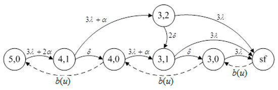
Figure 4. The state transition rate diagram of availability system 3.

We note that the states labeled (4,1) and (3,1) represent detection stages. The transition from state (4,1) to state (4,0), and from state (3,1) to state (3,0) indicate the detection of the respective faults.

Using similar argument led to the explicit expression for the steady-state availability, $A{v}_3$, which is given by:

$$A{v}_3=P_{5,0}+P_{4,0}+P_{3,0}=\left\{1+\frac{(3\lambda +2\alpha )[1-B^{*}(3\lambda +\alpha )]}{(3\lambda +\alpha )B^{*}(3\lambda +\alpha )}+\frac{\Phi [1-B^{*}(3\lambda )]}{3\lambda B^{*}(3\lambda )}\right\}{P}_{5,0}.$$

(19)

The detailed derivation of $A{v}_3$ is provided in Appendix C.

Special Cases

For availability system 3, by substituting $B^{*}(s)$ for three different repair time distributions—exponential, $k$-stage Erlang, and the deterministic distribution in Equation (19)—the following expressions for $A{v}_{3M}$, $A{v}_{3E},$ and $A{v}_{3D}$ were obtained:

$$A{v}_{3M}=\frac{3\lambda +2\alpha +\mu +{\Phi }_1}{\mu }{P}_{5,0},$$

$$A{v}_{3E}=1+\frac{(3\lambda +2\alpha )\left[{(k\mu +3\lambda +\alpha )}^k-{(k\mu )}^k\right]}{(3\lambda +\alpha ){(k\mu )}^k}+\frac{{\Phi }_2\left[{(k\mu +3\lambda )}^k-{(k\mu )}^k\right]}{3\lambda {(k\mu )}^k}{P}_{5,0},$$

$$A{v}_{3D}=1+\frac{(3\lambda +2\alpha )\left(e^{\raisebox{1ex}{$3\lambda +\alpha $}\!\left/ \!\raisebox{-1ex}{$\mu $}\right.}-1\right)}{3\lambda +\alpha }+\frac{{\Phi }_3\left(e^{\raisebox{1ex}{$3\lambda $}\!\left/ \!\raisebox{-1ex}{$\mu $}\right.}-1\right)}{3\lambda }{P}_{5,0},$$

where

$${\Phi }_1=\frac{(3\lambda +2\alpha )[(3\lambda +\alpha +\delta )(\mu +3\lambda +\alpha )-\delta \mu ]}{\mu (3\lambda +\alpha +\delta )},$$

$${\Phi }_2=\frac{(3\lambda +2\alpha )[(3\lambda +\alpha +\delta ){(k\mu +\lambda )}^k-\delta {(k\mu )}^k]}{(3\lambda +\alpha +\delta ){(k\mu )}^k},$$

$${\Phi }_3=\frac{(3\lambda +2\alpha )\left[(3\lambda +\alpha +\delta )e^{\raisebox{1ex}{$3\lambda +\alpha $}\!\left/ \!\raisebox{-1ex}{$\mu $}\right.}-\delta \right]}{3\lambda +\alpha +\delta }.$$

5. Comparison of the Three Availability Systems

In this section, we compare the three availability systems in terms of $Av$ and cost/benefit ratios for three different repair time distributions, where benefit is defined as $Av$. Basically, the following values of various parameters were set as follows:

$$\frac{1}{\lambda }=1000\mathrm{days},\frac{1}{\alpha }=2000\mathrm{days},\frac{1}{\mu }=10\mathrm{days},\frac{1}{\delta }=\frac{10}{24}\mathrm{day},$$

or

$$\lambda =0.001,\alpha =0.0005,\mu =0.1,\delta =2.4.$$

5.1. Comparisons of Availability for the Three Systems

First, the following three cases were performed to obtain a comparison between the $Av$’s of the three availability systems when the three repair time distributions were set to be exponential, three-stage Erlang, and deterministic, respectively.

Case 1. We fixed $\mu =0.1$, $\delta =2.4$, and varied the values of $\lambda$ from 0.001 to 0.02.

Case 2. We fixed $\lambda =0.001$, $\alpha =0.0005$, $\delta =2.4$, and varied the values of $\mu$ from 0.05 to 0.16.

Case 3. We fixed $\lambda =0.001$, $\alpha =0.0005$, $\mu =0.1$, and varied the values of $\delta$ from 1 to 10.

Numerical results of the $A{v}_{iM}$, $A{v}_{iE}$, and $A{v}_{iD}$ for each availability system i (i = 1, 2, 3) are shown in Table 1, Table 2 and Table 3 for cases 1–3, respectively. From Table 1, Table 2 and Table 3, it can be observed that system 1 was the best system based on the availability comparison. However, note that each system consumed different costs during their construction; therefore, the cost/Av ratio was fairer than Av as the criterion for comparing the three systems.

Table 1. Comparison of the availability systems 1, 2, 3 for Av ($\alpha =\lambda /2,\mu =0.1,\delta =2.4$).

Range of $\mathit{\lambda }$	Result
1. Exponential $0.001<\lambda <0.001477$ $0.001477<\lambda <0.013881$ $0.013881<\lambda <0.02$	$A{v}_{1M}>A{v}_{2M}>A{v}_{3M}$ $A{v}_{1M}>A{v}_{3M}>A{v}_{2M}$ $A{v}_{1M}>A{v}_{2M}>A{v}_{3M}$
2. Three-stage Erlang $0.001<\lambda <0.002459$ $0.002459<\lambda <0.010156$ $0.010156<\lambda <0.02$	$A{v}_{1E}>A{v}_{2E}>A{v}_{3E}$ $A{v}_{1E}>A{v}_{3E}>A{v}_{2E}$ $A{v}_{1E}>A{v}_{2E}>A{v}_{3E}$
3. Deterministic $0.001<\lambda <0.003956$ $0.003956<\lambda <0.007653$ $0.007653<\lambda <0.02$	$A{v}_{1D}>A{v}_{2D}>A{v}_{3D}$ $A{v}_{1D}>A{v}_{3D}>A{v}_{2D}$ $A{v}_{1D}>A{v}_{2D}>A{v}_{3D}$

Table 2. Comparison of the availability systems 1, 2, 3 for Av ($\lambda =0.001,\alpha =\lambda /2,\delta =2.4$).

Range of $\mathit{\mu }$	Result
1. Exponential $0.05<\mu <0.083678$ $0.083678<\mu <0.16$	$A{v}_{1M}>A{v}_{3M}>A{v}_{2M}$ $A{v}_{1M}>A{v}_{2M}>A{v}_{3M}$
2. Three-stage Erlang $0.05<\mu <0.067598$ $0.067598<\mu <0.16$	$A{v}_{1E}>A{v}_{3E}>A{v}_{2E}$ $A{v}_{1E}>A{v}_{2E}>A{v}_{3E}$
3. Deterministic $0.05<\mu <0.057929$ $0.057929<\mu <0.16$	$A{v}_{1D}>A{v}_{3D}>A{v}_{2D}$ $A{v}_{1D}>A{v}_{2D}>A{v}_{3D}$

Table 3. Comparison of the availability systems 1, 2, 3 for Av ($\lambda =0.001,\alpha =\lambda /2,\mu =0.1$).

Range of $\mathit{\delta }$	Result
1. Exponential $1<\delta <3.350022$ $3.350022<\delta <10$	$A{v}_{1M}>A{v}_{2M}>A{v}_{3M}$ $A{v}_{1M}>A{v}_{3M}>A{v}_{2M}$
2. Three-stage Erlang $1<\delta <4.980970$ $4.980970<\delta <10$	$A{v}_{1E}>A{v}_{2E}>A{v}_{3E}$ $A{v}_{1E}>A{v}_{3E}>A{v}_{2E}$
3. Deterministic $1<\delta <6.611954$ $6.611954<\delta <10$	$A{v}_{1D}>A{v}_{2D}>A{v}_{3D}$ $A{v}_{1D}>A{v}_{3D}>A{v}_{2D}$

5.2. Comparisons of the Cost/Benefit Ratios for the Three Availability Systems

Next, we considered that the systems with different power capacities may have different costs. These costs should be considered when different systems are fairly compared. The capacity-proportional costs for the primary components and warm standby components are listed in Table 4. From Table 4, the cost for each availability system i (i = 1, 2, 3) was calculated and are shown in Table 5.

Table 4. The size-proportional cost for the primary and warm standby components.

Component	Cost (in $)	Component	Cost (in $)
Primary 30 MW	$30\times {10}^6$	Standby 30 MW	$24\times {10}^6$
Primary 15 MW	$15\times {10}^6$	Standby 15 MW	$12\times {10}^6$
Primary 10 MW	$10\times {10}^6$	Standby 10 MW	$8\times {10}^6$

Table 5. The cost of each availability system.

Availability Systems	Cost (in $)
Availability System 1	$54\times {10}^6$
Availability System 2	$42\times {10}^6$
Availability System 3	$46\times {10}^6$

Let $C_i$ denote the cost of availability system $i$, and $B{F}_i$ be the benefit of availability system $i$, where $B{F}_i$ is $A{v}_i$ and $i=1,2,3$. Based on the cost/benefit ratio, comparisons of the three systems were made. We ranked the three availability systems under specific values of system parameters $\lambda$, $\mu$, and $\delta$, as well as the costs given in Table 5. The results of the rank (cost/benefit) are shown in Table 6, Table 7 and Table 8 for ranges of $\lambda$, $\mu$, and $\delta$, respectively. We can easily observe from Table 6, Table 7 and Table 8 that system 2 was the best model when considering the cost/Av value for most cases. It can be observed that this system 2 is the dominant optimal model in terms of the cost/Av value independent of both the distributions of the repair time and the ranges of $\lambda$, $\mu$, and $\delta$.

Table 6. Rank of $C_i/A{v}_i$ for $\alpha =\lambda /2,\mu =0.1,\delta =2.4$.

Range of $\mathit{\lambda }$	Rank (${\mathit{C}}_{\mathit{i}}\mathbf{/}\mathit{A}{\mathit{v}}_{\mathit{i}}$)
1. Exponential $0.001<\lambda <0.024967$ $00.024967<\lambda <0.049336$ $0.049336<\lambda <0.08$	$\mathrm{System}1>\mathrm{System}3>\mathrm{System}2$ $\mathrm{System}3>\mathrm{System}1>\mathrm{System}2$ $\mathrm{System}3>\mathrm{System}2>\mathrm{System}1$
2. Three-stage Erlang $0.001<\lambda <0.025245$ $0.025245<\lambda <0.054168$ $0.054168<\lambda <0.08$	$\mathrm{System}1>\mathrm{System}3>\mathrm{System}2$ $\mathrm{System}3>\mathrm{System}1>\mathrm{System}2$ $\mathrm{System}3>\mathrm{System}2>\mathrm{System}1$
3. Deterministic $0.001<\lambda <0.026111$ $0.026111<\lambda <0.058190$ $0.058190<\lambda <0.08$	$\mathrm{System}1>\mathrm{System}3>\mathrm{System}2$ $\mathrm{System}3>\mathrm{System}1>\mathrm{System}2$ $\mathrm{System}3>\mathrm{System}2>\mathrm{System}1$

Table 7. Rank of $C_i/A{v}_i$ for $\lambda =0.001,\alpha =\lambda /2,\delta =2.4$.

Range of $\mathit{\mu }$	Rank (${\mathit{C}}_{\mathit{i}}\mathbf{/}\mathit{A}{\mathit{v}}_{\mathit{i}}$)
1. Exponential $0.001<\mu <0.001971$ $0.001971<\mu <0.003728$ $0.003728<\mu <0.16$	$\mathrm{System}3>\mathrm{System}2>\mathrm{System}1$ $\mathrm{System}3>\mathrm{System}1>\mathrm{System}2$ $\mathrm{System}1>\mathrm{System}3>\mathrm{System}2$
2. Three-stage Erlang $0.001<\mu <0.001822$ $0.001822<\mu <0.003753$ $0.003753<\mu <0.16$	$\mathrm{System}3>\mathrm{System}2>\mathrm{System}1$ $\mathrm{System}3>\mathrm{System}1>\mathrm{System}2$ $\mathrm{System}1>\mathrm{System}3>\mathrm{System}2$
3. Deterministic $0.001<\mu <0.001718$ $0.001718<\mu <0.003666$ $0.003666<\mu <0.16$	$\mathrm{System}3>\mathrm{System}2>\mathrm{System}1$ $\mathrm{System}3>\mathrm{System}1>\mathrm{System}2$ $\mathrm{System}1>\mathrm{System}3>\mathrm{System}2$

Table 8. Rank of $C_i/A{v}_i$ for $\lambda =0.001,\alpha =\lambda /2,\mu =0.1$.

Range of $\mathit{\delta }$	Rank (${\mathit{C}}_{\mathit{i}}\mathbf{/}\mathit{A}{\mathit{v}}_{\mathit{i}}$)
1. Exponential $0.001<\delta <0.014386$ $0.014386<\delta <10$	$\mathrm{System}3>\mathrm{System}1>\mathrm{System}2$ $\mathrm{System}1>\mathrm{System}3>\mathrm{System}2$
2. Three-stage Erlang $0.001<\delta <0.014379$ $0.014379<\delta <10$	$\mathrm{System}3>\mathrm{System}1>\mathrm{System}2$ $\mathrm{System}1>\mathrm{System}3>\mathrm{System}2$
3. Deterministic $0.001<\delta <0.014375$ $0.014375<\delta <10$	$\mathrm{System}3>\mathrm{System}1>\mathrm{System}2$ $\mathrm{System}1>\mathrm{System}3>\mathrm{System}2$

6. Conclusions

This study first exploited the supplementary variable technique to derive the steady-state availability $Av$ of three availability systems with warm standby components, fault detection delays, and general repair times. Next, for each availability system, the expressions for the $Av$ of three different repair time distributions, namely exponential, three-stage Erlang, and deterministic, were explicitly derived. We demonstrated that the first system generalized Trivedi’s two-component system with a fault detection delay. Finally, we performed a numerical investigation in terms of both Av and the cost/Av for three availability systems and ranked the three systems based on Av and the cost/Av for three different repair time distributions. The numerical results demonstrated that availability system 2 outperformed the other two systems based on the criterion of cost/Av, which is fairer than using criterion Av for most cases. In a real-life situation, if the exponential distributions are reasonable for modeling the failures and detection delay times, the results of this paper can provide decision-makers with a practical tool for designing systems.

References

- Trivedi, K.S. Probability and Statistics with Reliability, 2nd ed.; John Wiley and Sons: Hoboken, NJ, USA, 2002. [Google Scholar]
- Cox, D.R. The analysis of non-Markovian stochastic processes by the inclusion of supplementary variables. Math. Proc. Camb. Philos. Soc. 1955, 51, 433–441. [Google Scholar] [CrossRef]
- Hokstad, P. A supplementary variable technique applied to the M/G/1 queue. Scand. J. Stat. 1975, 2, 95–98. [Google Scholar]
- Gupta, U.C.; Rao, T.S.S.S. A recursive method compute the steady state probabilities of the machine interference model: (M/G/1)/K. Comput. Oper. Res. 1994, 21, 597–605. [Google Scholar] [CrossRef]
- Gupta, U.C.; Rao, T.S.S.S. On the M/G/1 machine interference model with spares. Eur. J. Oper. Res. 1996, 89, 164–171. [Google Scholar] [CrossRef]
- Ke, J.-C.; Wang, K.-H. A recursive method for the N policy G/M/1 queueing system with finite capacity. Eur. J. Oper. Res. 2002, 142, 577–594. [Google Scholar] [CrossRef]
- Zhang, Y.L.; Wu, S. Reliability analysis for a k/n (F) system with repairable repair-equipment. Appl. Math. Model. 2009, 33, 3052–3067. [Google Scholar] [CrossRef]
- Shakuntla, S.; Lal, A.K.; Bhatia, S.S.; Singh, J. Reliability analysis of Polytube industry using supplementary variable technique. Appl. Math. Comput. 2011, 218, 3981–3992. [Google Scholar] [CrossRef]
- Wang, K.-H.; Su, J.-H.; Yang, D.-Y. Analysis and optimization of an M/G/1 machine repair problem with multiple imperfect coverage. Appl. Math. Comput. 2014, 242, 590–600. [Google Scholar] [CrossRef]
- Ke, J.-C.; Liu, T.-H.; Yang, D.-Y. Modeling of machine interference problem with unreliable repairman and standbys imperfect switchover. Reliab. Eng. Syst. Saf. 2018, 174, 12–18. [Google Scholar] [CrossRef]
- Wang, K.-H.; Pearn, W.L. Cost benefit analysis of series systems with warm standby components. Math. Methods Oper. Res. 2003, 58, 247–258. [Google Scholar] [CrossRef]
- Wang, K.-H.; Chiu, L.-W. Cost benefit analysis of availability systems with warm standby units and imperfect coverage. Appl. Math. Comput. 2006, 172, 1239–1256. [Google Scholar] [CrossRef]
- Wang, K.-H.; Chen, Y.-J. Comparative analysis of availability between three systems with general repair times, reboot delay and switching failures. Appl. Math. Comput. 2009, 215, 384–394. [Google Scholar] [CrossRef]
- Singh, V.V.; Singh, S.B.; Ram, M.; Goel, C.K. Availability, MTTF and cost analysis of a system having two units in series configuration with controller. Int. J. Syst. Assur. Eng. Manag. 2013, 4, 341–352. [Google Scholar] [CrossRef]
- Yu, H.; Chu, C.; Chatelet, E. Availability optimization of a redundant system through dependency modeling. Appl. Math. Model. 2014, 38, 4574–4585. [Google Scholar] [CrossRef]
- Ke, J.-C.; Lee, S.-L.; Hsu, Y.-L. On a repairable system with detection, imperfect coverage and reboot: Bayesian approach. Simul. Model. Pract. Theory 2008, 16, 353–367. [Google Scholar] [CrossRef]
- Kleyner, A.; Volovoi, V. Application of petri nets to reliability prediction of occupant safety systems with partial detection and repair. Reliab. Eng. Syst. Saf. 2010, 95, 606–613. [Google Scholar] [CrossRef]
- Ke, J.-C.; Liu, T.-H. A repairable system with imperfect coverage and reboot. Appl. Math. Comput. 2014, 246, 148–158. [Google Scholar] [CrossRef]
© 2020 by the authors. Licensee MDPI, Basel, Switzerland. This article is an open access article distributed under the terms and conditions of the Creative Commons Attribution (CC BY) license (http://creativecommons.org/licenses/by/4.0/).