Article

Anticipating the Length of Employees’ Working Time

by
Paulina Kostrzewa-Demczuk
1,* and
Magdalena Rogalska
2
1
Department of Building and Architecture, Kielce University of Technology, al. Tysiąclecia Państwa Polskiego 7, 25-314 Kielce, Poland
2
Department of Building and Architecture, Lublin Technical University, ul. Nadbystrzycka 40, 20-618 Lublin, Poland
*
Author to whom correspondence should be addressed.
Symmetry 2020, 12(3), 413; https://doi.org/10.3390/sym12030413
Submission received: 4 December 2019 / Revised: 15 January 2020 / Accepted: 15 January 2020 / Published: 5 March 2020

Abstract

:
Asymmetry of employee productivity is an important issue when planning production work. Estimated time to complete the work depends on many factors, such as employee experience, qualifications, and efficiency of brigades and subcontractors, accidents, unreliable suppliers, material shortages, the need for correction work, fatigue, stress, etc. The paper presents the statistical method—Multivariate Method of Statistical Models—MMSM. It enables the assessment of the impact on the duration of works of its characteristic variables and the prediction of the duration of individual orders. In order to carry out the multi-criteria method (MMSM) analysis, the employees’ working time was measured at the newly opened steel structure production plant in Kielce. The results of the analyses clearly show that thanks to the method used, quick and accurate prediction of employees’ work efficiency is possible. In the analyzed case, the best forecast was obtained using the method of automatic neural networks, where the MAPE error = 0.02%.

1. Introduction

Planning production works is an extremely important issue, which depends on the material delivery schedule, transport schedule, employment schedule, proper use of available work stations and machines, and many others [1]. Production ventures are exposed to various risk factors that can disturb the pre-planned time for the execution of the element. The most common risk factors are [2,3]: different employee experience, qualifications and performance of brigades and subcontractors, accidents, unreliable suppliers, material shortages, the need for correction work, fatigue, stress, etc. Beck and Shen even worked on the impact of presidential elections on employee productivity [4]. The variability of the environment in which the project is carried out is a source of uncertainty and risk. This risk relates mainly to the time, cost, and quality.
Production plants set average working time standards for the worker or the number of working hours to complete the item. However, these are averaged times, often not mapping in reality. Production schedules often turn out to be divergent with production practice and are the reason for delays in deliveries to contractors [5] which is associated with contractual penalties for failure to meet deadlines.
Today’s computing power creates opportunities for performing complex computational operations in a short time, and thus for creating completely new computational methods that are useful in the issue of scheduling. Many researchers deal with the subject of work efficiency and methods of its estimation or planning [6]. Research was carried out to determine the impact on work efficiency, including: fatigue and breaks [7,8], age of employees [9], accidents at work [3], motivating factors for work [10], and even the role of religion or sexuality of the employee [11].
The work presents a methodology for improving the planning of production works and determining their time, taking into account various factors affecting the implementation of production. The time of making a single element is the most important issue necessary for the correct control and production control. In Materials and Methods, the multi-criteria method (MMSM) is shown. Using this, it is possible to determine the best mapping of production time, depending on the size of the order, the type of performed elements, employee experience, equipment failure, and many other factors. The next section compiles the results of the tests carried out. In the Discussion section, the results of the analyzes are summarized and their usefulness in the forecast of employee work time results is assessed. The next section of the article summarizes the conclusions of the article.
The purpose of the work is to generate a regression formula showing the impact on the duration of works of certain characteristic variables for this process. It will determine the number of pieces of the produced item will be manufactured in the working hours, thanks to which it will be possible to predict the duration of work for a specific order.

2. Materials and Methods

In order to conduct the Multivariate Method of Statistical Models (MMSM) analysis, the employees’ working time was measured at the newly opened steel structure production plant in Kielce in 2019. The measuring plant employed 8 employees as welder-grinders. Therefore, it should be emphasized that in addition to welding work, each employee also performs grinding works, which are time consuming.
Eight employees of differing age and professional experience were observed for four days. The measurements performed concerned employee performance (dependent variable), which was determined in pieces of the welded element per hour of effective work (Table 1). Employee performance depended on independent variables: experience, the number of effective working hours, the number of elements made at that time, equipment failure rate, average hall temperature, manufacturing errors and partly associated grinding time, or employee well-being.
The employees work eight hours a day, from 6:00 to 14:00, during which they have an 0.5 h lunch break. The effective working hours were defined as the time during the day spent on welding, after counting the lunch break, this time can be a maximum of 7.5 h.
The scope of work for these workers include: preparatory work of the workplace, replacement of welding gases and welding wire, initial dimensional control of prepared elements, care for entrusted equipment and tools, welding, and grinding of produced elements. It happens that an employee stay longer in work, or leaves the workplace earlier (after previous agreement with boss). Depending on the self-organization of the workplace and experience, employees achieve different times.
The time of making a single element (steel structure) depends on its size, complexity, number of welded joints and their types, welding methods, and many others. In order to limit the number of independent variables affecting employee performance, the research was conducted on employees producing the same type of steel structure and using the MAG welding method. All employees used welding and grinding machines from the same company.
The number of elements made during one work shift by one employee was assumed to be approximately 0.25, because employees did not always finish the last produced element. Such an element was left in the position and work began the next day.
During welding processes, numerous pollutants in the form of dust and gases are emitted, as well as optical radiation, high temperature, electromagnetic field and noise, which have a negative impact on human health and its work efficiency. Favorable working conditions of welders led to greater process efficiency. Poor working conditions led to frequent fluctuations in quality and sometimes work efficiency. Every day, employees were asked to rate their well-being and health on a scale of 1–5. 1: very bad, 2: bad, 3: normal, 4: good, 5: very good.

Methods

The Multivariate Method of Statistical Models (MMSM) is a new methodology for forecasting project implementation time. It allows you to create schedules taking into account real conditions, not averaged. The method is based on the computational analysis of prognostic methods: multiple regression, multi-naming adaptive regression using spline functions, generalized additive models, artificial neural networks, support vectors. and integrated autoregression. Conducting calculations involves conducting prognostic analyzes, from which the best fit to real data is then selected based on the least prognostic error. The method was developed by M. Rogalska [12] and is successfully used to predict the times of construction works.
At the initial stage of the analysis, it is necessary to determine the type of distribution of individual variables. Normal distribution Gaussian distribution is the most common type of empirical distribution. It results from the fact that many phenomena, especially natural ones, are shaped according to such a distribution [13]. To determine the normality of the distribution, the Shapiro-Wilk test is performed. It is the preferred test of normality because of its high power compared to other tests. Using the Shapiro-Wilk test, it is possible to check if the variables have distributions close to the normal distribution [14]. The Shapiro-Wilk test statistic value for 32 cases should be a minimum of 0.930 for the distribution to be classified as normal.
The next step is to check the correlation between variables, so you can eliminate strongly related variables that can affect the disturbance or distortion of the analysis.
Based on the collected data (Table 1), analyses were performed using such computational methods as multiple regression forecasting (MR (Multiple Regresion), forecasting using multimodal adaptive regression using glued functions—MARSplines (Multivariate Adaptive Regression Splines), forecasting using generalized models additive—GAM (Generalized Additive Models), as well as the method of Automatic Neural Networks—NN (Neural Networks).
Forecasting by means of multiple regression method, it aims to quantify the relationships between many independent (explanatory) and dependent (criterion, explained) variables [15,16]. The purpose of building and analyzing the multiple redression model is to examine the existence of relationships between variables and the effect of Xi variables on the Y variable (in this case, “employee performance”). The condition for the correctness of the model is: no strong correlation between independent variables, a greater number of observations than the number of parameters to be estimated, independent variables cannot be a linear combination of other independent variables.
Forecasting with the use of multi-naming adaptive regression methods using spline functions is known as MARSplines. The MARS method is one of the many tools of statistical data mining [17], used, among others, to solve regression problems. As a non-parametric model, it does not require assumptions about the shape of the functional relationship between dependent and independent variables. This relationship is determined as a linear combination of base functions based solely on the information contained in the input data. Data is divided into areas in which separate regression functions are independently defined. This tool is especially valuable with more dimensions and large data sets, with complex relationships between them.
Forecasting by the method of generalized additive models is known as GAM. Generalized additive models, in short, GAM, were developed in 1990 by Hastie and Tibshirani [18,19,20] who proposed estimation for multidimensional variables by means of additive approximation of the regression function, replacing the linear function of explanatory variables with additive “nonparametric” functions, which can be estimated, for example, by smoothed cubic spline functions. In the case of generalized additive models, instead of a combination of linear predictors, we used a nonparametric function obtained by applying smoothing to the scatter chart of partial residuals (for transformed values of the dependent variable).
Forecasting with the NN method allows obtaining very good forecast results [12]. It involves the processing of data by neurons grouped into layers. Appropriate results are obtained thanks to the learning process, which consists of modifying the weights of those neurons that are responsible for the error. Neural networks are resistant to damage, to incorrect or incomplete information [12]. They can operate efficiently even when some of its elements are damaged and some of the data is lost. They are best suited for solving a class of tasks where writing a normal program is very difficult or impossible, e.g., due to the lack of a known algorithm.
The regression line expresses the best prediction of the dependent variable for given independent variables. However, nature is rarely perfectly predictable and we usually deal with deviations of the measurement points from the regression line. The deviation of a given point on the graph from the regression line (i.e., its predicted value) is called the “residual” value. During the individual analyses, their correctness was checked and assessed by means of the autocorrelation check and partial autocorrelation of residues, as well as fit charts. All analyses, in the last phase of work, were subjected to the MAPE error test. The MAPE (Mean Absolute Percentage Error) error [12,21] is the average absolute percentage error that is made when forecasting based on a specific model. This parameter is known by analyzing the accuracy of forecasts constituting the basis for building the estimation model. It informs about the average size of measured errors. It follows that the smaller the MAPE, the better. The error is expressed by the formula:
M A P E = 1 T n   i = T n T | Y i Y i p | Y i
where: T—number of the last moment/period for which the forecast was checked; N—number of the last known observation of the forecast variable; Yi—actual value of the variable in period i; Yip—projected value of the variable in period i.

3. Results

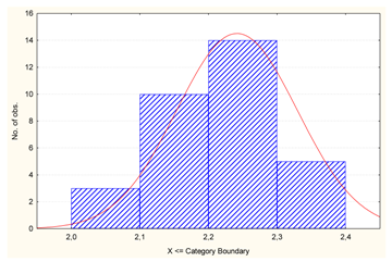
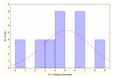
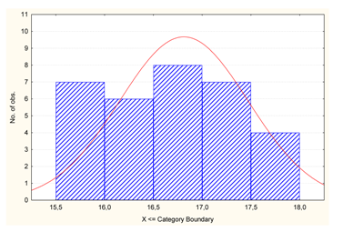
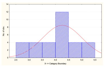
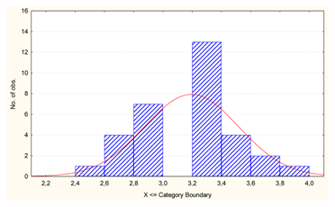
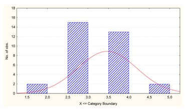
The variables were subjected to the normality test. The results (Table 2) show that most of the data has a normal distribution. In contrast, temperature and well-being are variables with a distribution close to normal.
Correlations between variables were examined. The results indicate a relationship between variables (Table 3). Correlations mean that the independent variable has an impact on the independent variable. In practice, this means that employee performance largely depends on the number of components made, employee experience, and the time of grinding. The most correlated independent variables are “number of items made” and “employee experience”. Some methods, such as multiple reflection, require variables not to be strongly correlated. Therefore, one of these variables will need to be excluded from the analysis, because it can generate a larger error or completely prevent calculations.

3.1. Multiple Regresion Method

In the multiple regression method, the independent variable “number of elements made” was excluded from the calculations, because it was very strongly correlated with the dependent variable “employee performance” and the variable “employee experience” (Figure 1).
The use of two independent variables that are predictors and strongly linearly correlated with each other may have a negative impact on the analysis. In such a situation, independent variables will not introduce a significant dependence to the regression pattern, only a distortion.

3.1.1. MR1

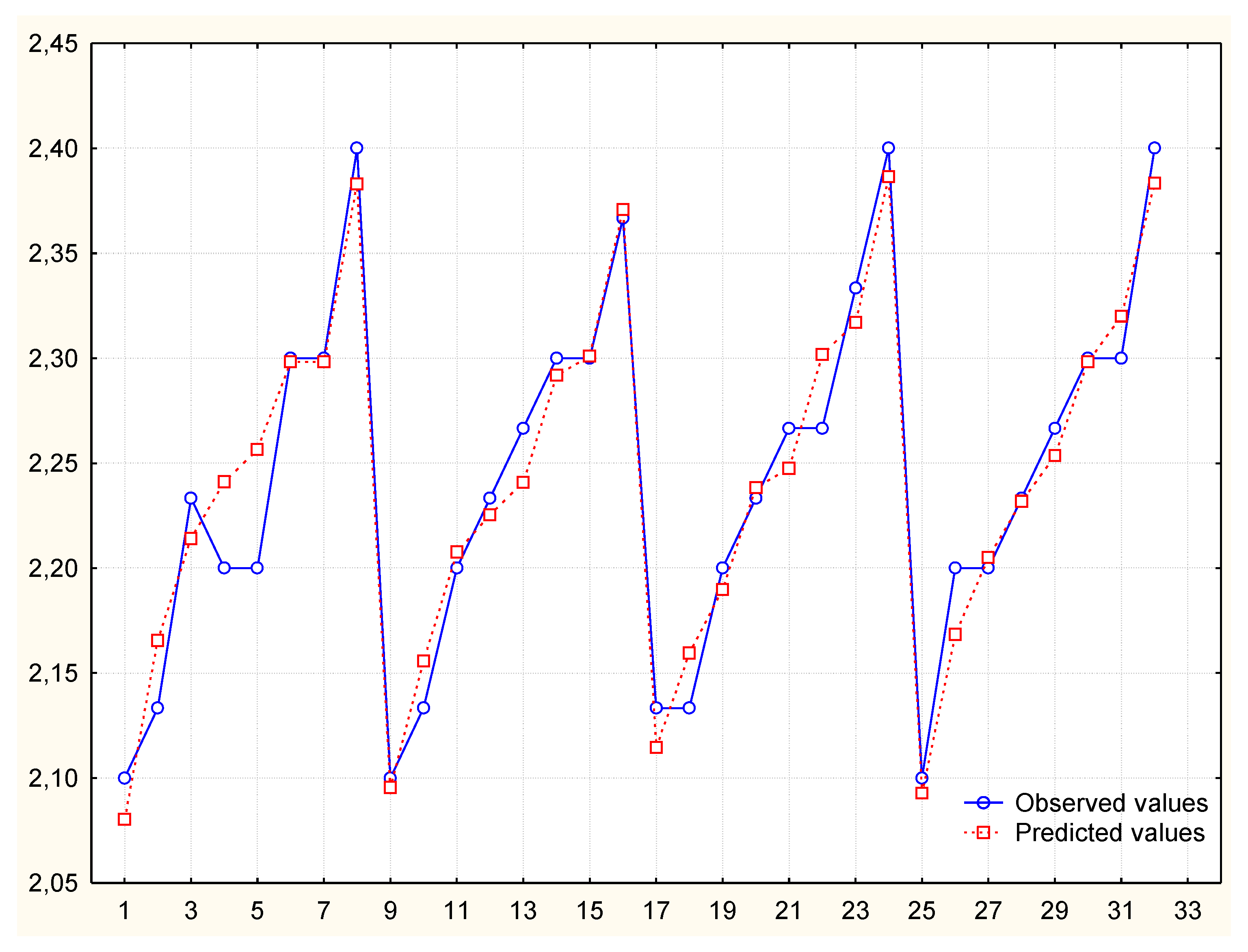
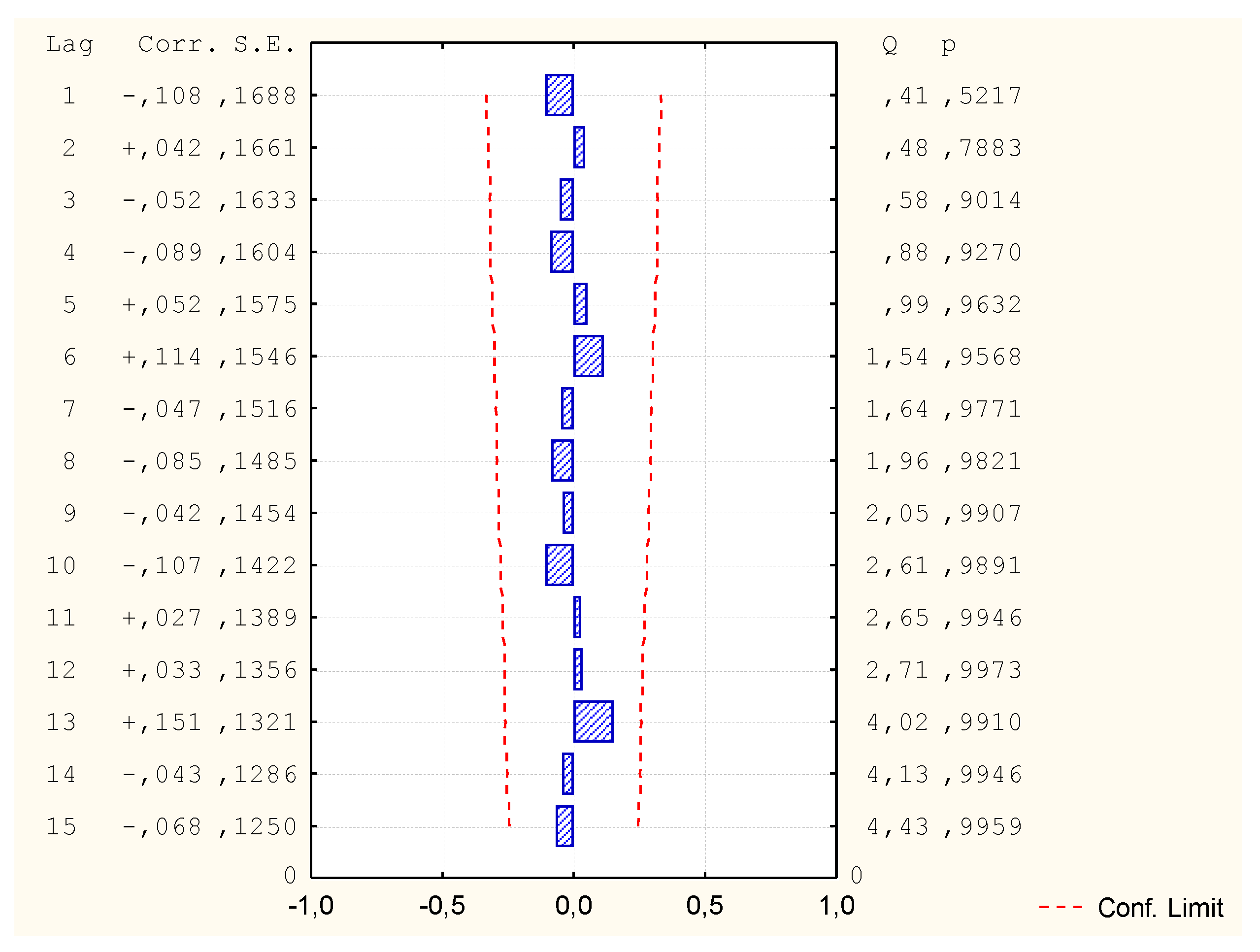
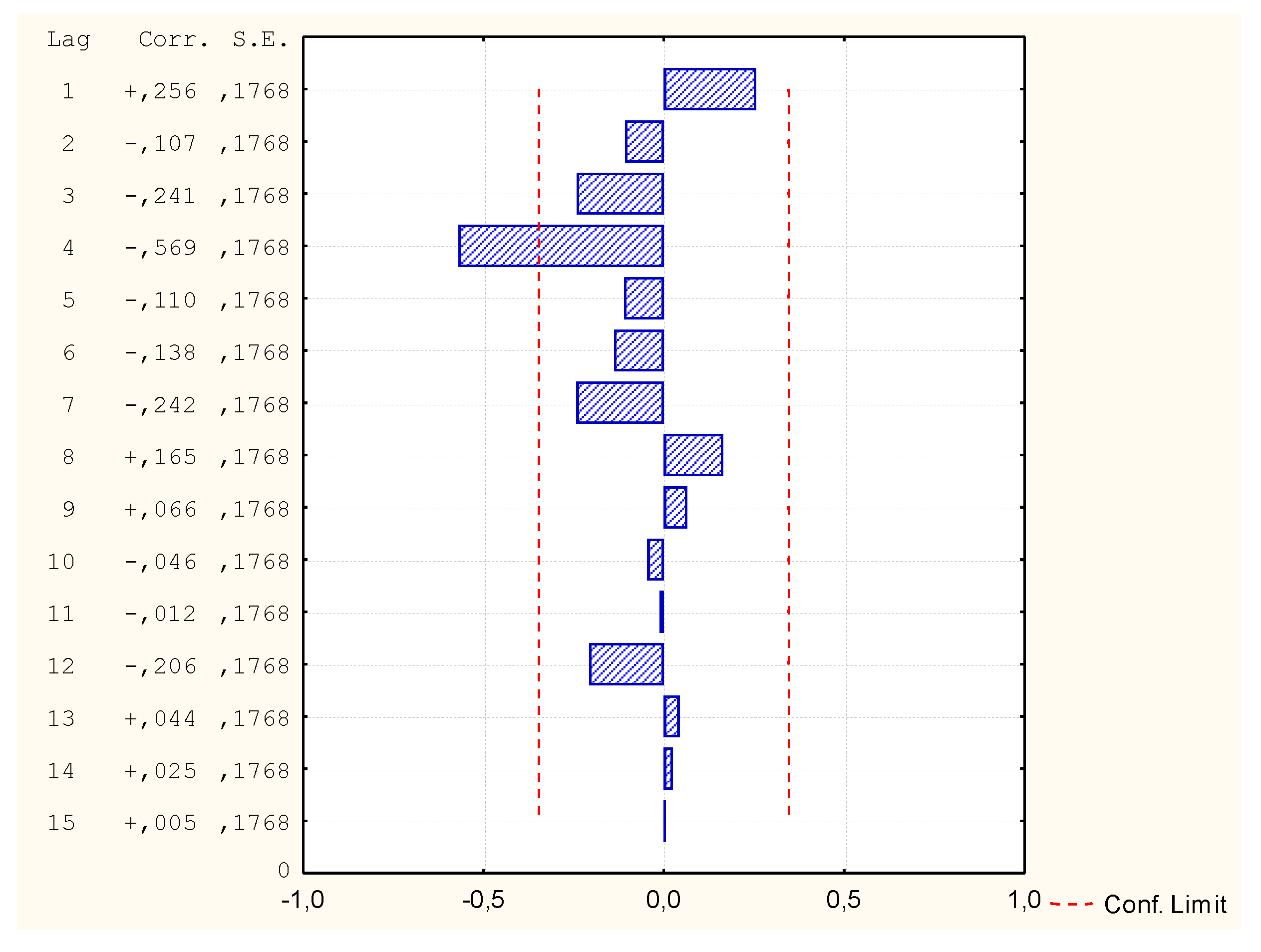
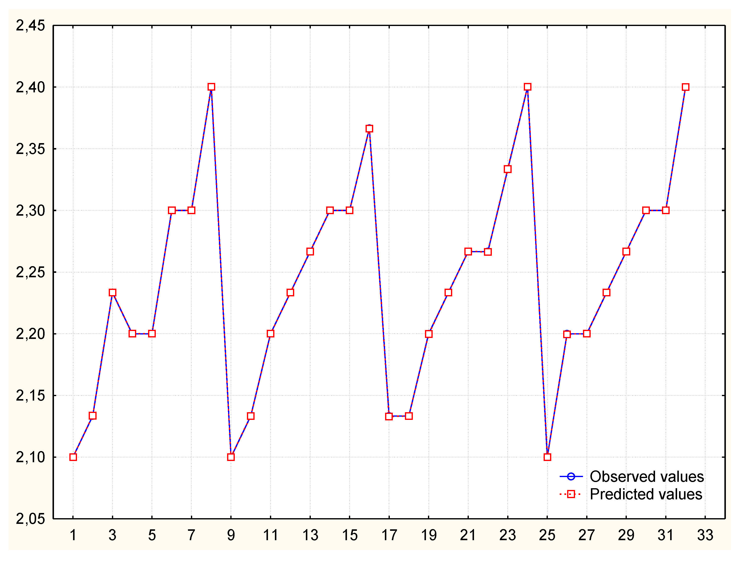
Table 4 is a summary of the MR1 analysis. Independent variables were used for the analysis: v2, v5, v6, v7 (Figure 2, Figure 3 and Figure 4). Based on the generated calculations, it was possible to determine a regression formula that would allow prediction.
MAPE error [%] = 0.72.
Based on the calculations and analysis of their results, the correctness of the adopted model is confirmed.

3.1.2. MR2

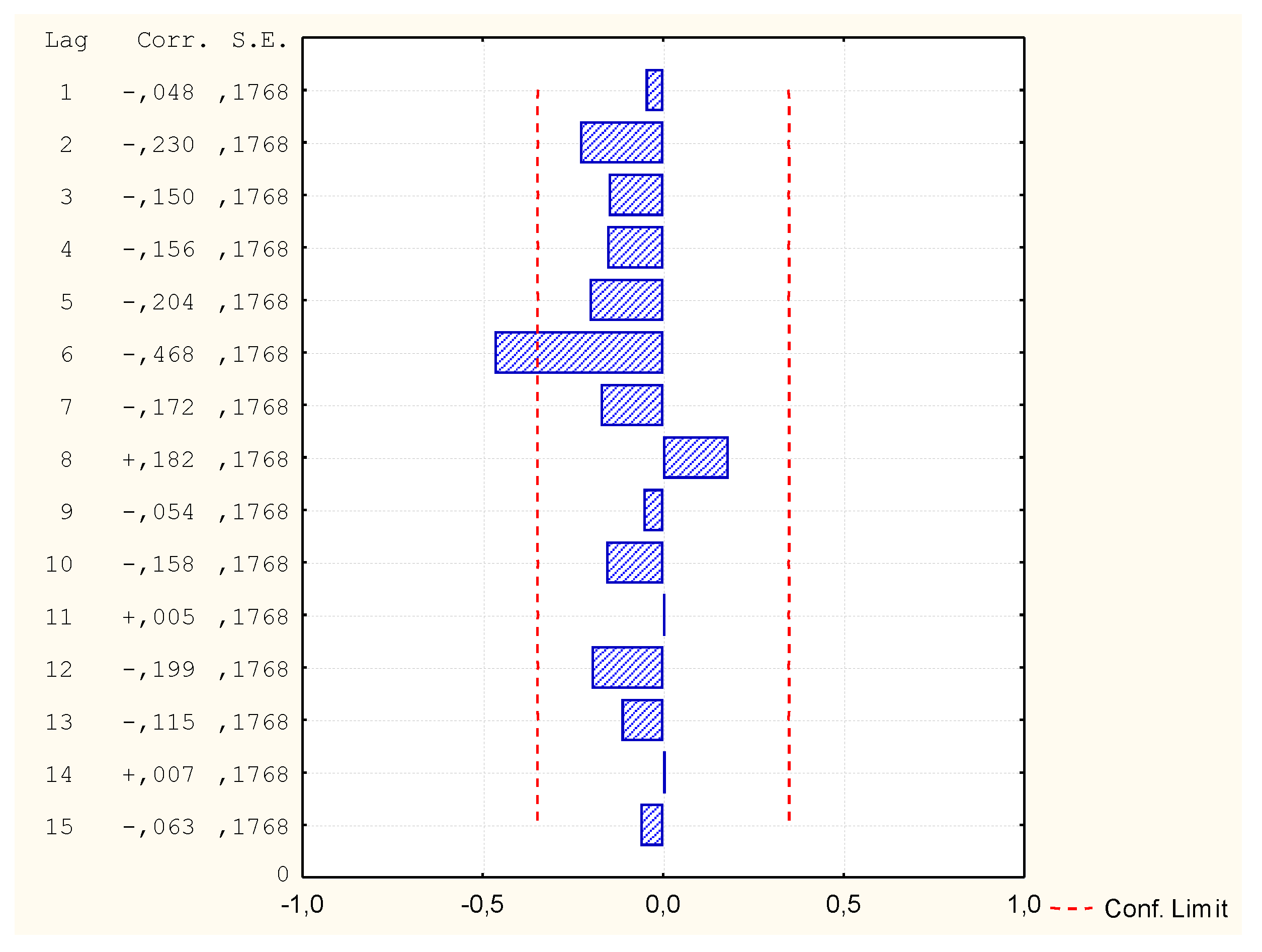
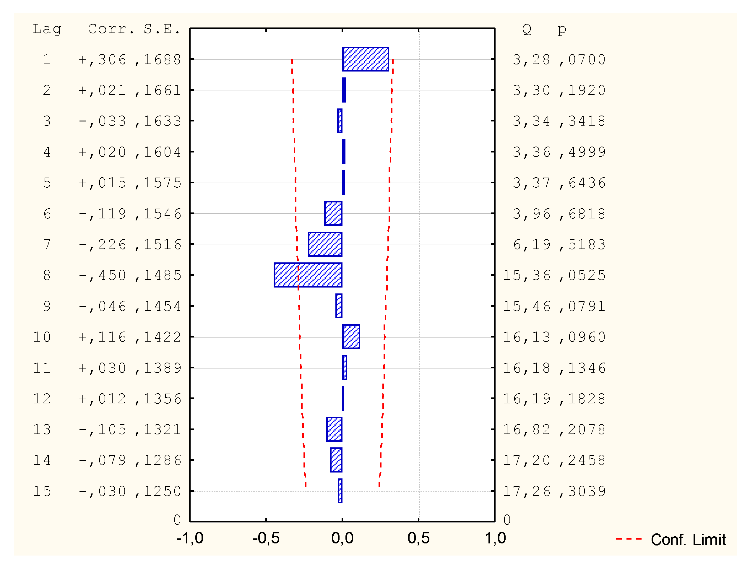
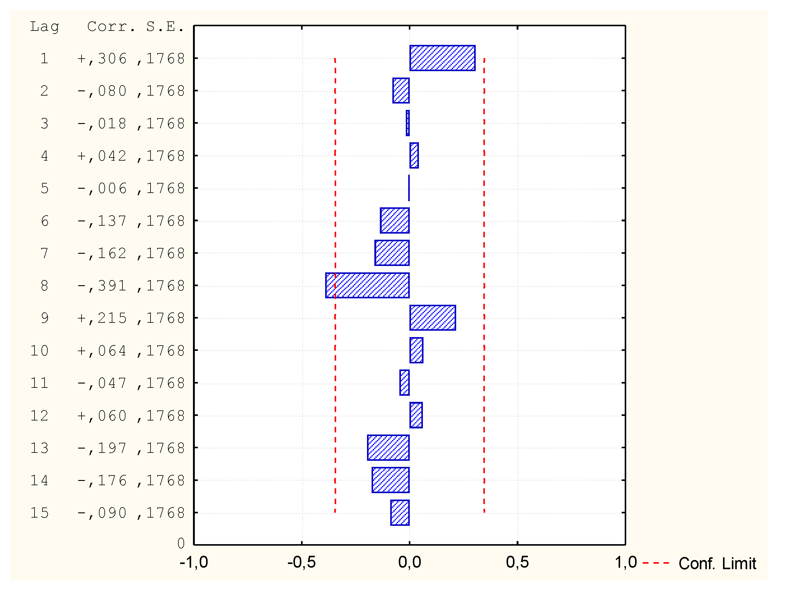
To obtain a better prediction, the independent variable “number of elements made” was modified so that its distribution was normal. The variable v3 was logarithmized and then used in the analysis (Table 5). Despite the good mapping on the graph of predicted and observed values, it turned out that in comparison the values of autocorrelation of residues and autocorrelation of partial residues exceed the limit. Thus, the model is not correct (Figure 5, Figure 6 and Figure 7) and its analysis and calculation of the MAPE error was not continued.

3.2. Multivariate Adaptive Regression Splines Method

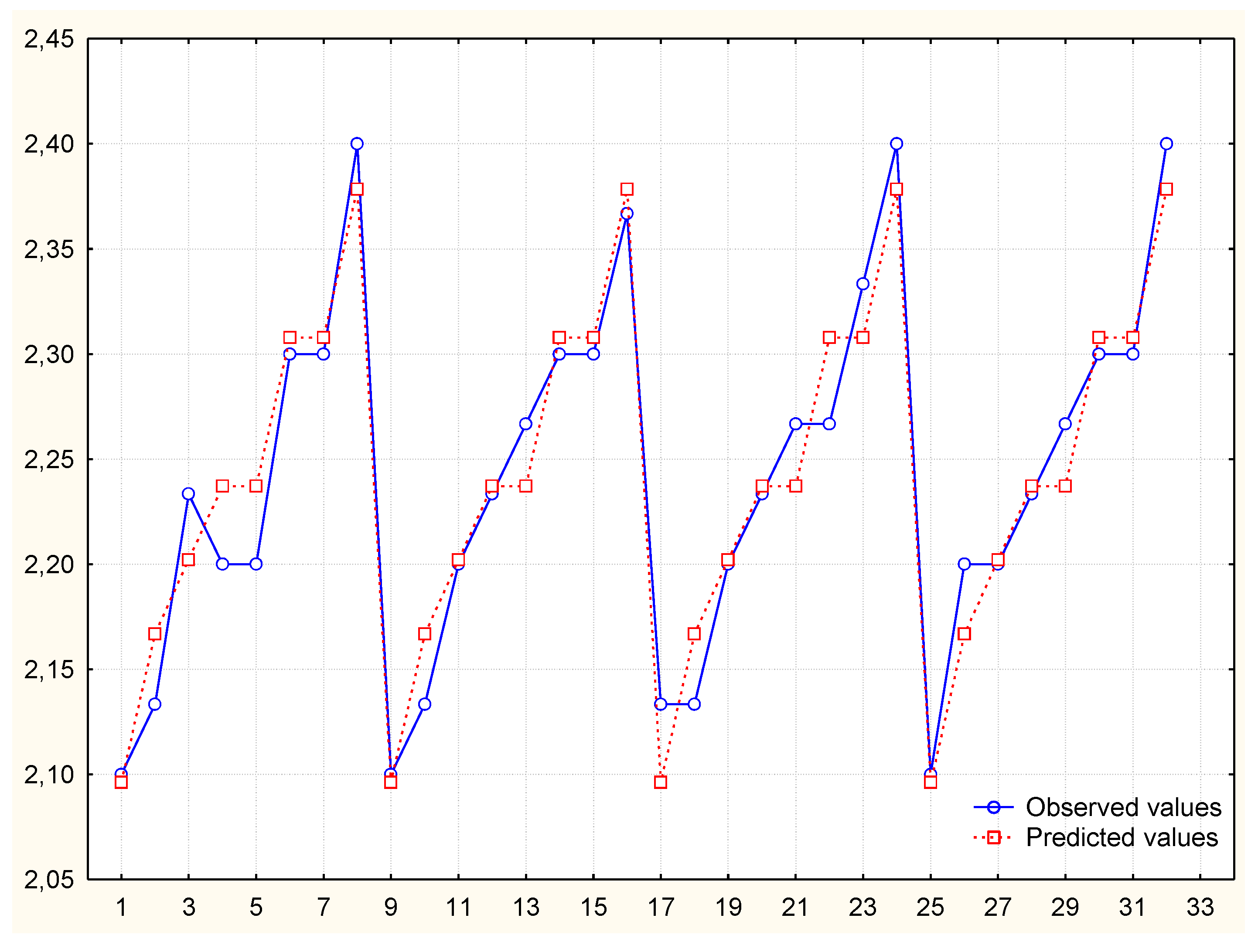
The MARSplines method itself rejects correlated variables during analysis. Thus, in this case, all available independent variables were used for the calculation (Table 6, Table 7 and Table 8). The forecast and observed values chart does not coincide very well, but is satisfactory. No discrepancies were detected in the values of the residue autocorrelation and autocorrelation functions particle residue, so the model as well as the regression pattern is considered to be correct (Figure 8, Figure 9 and Figure 10). The last step of the analysis was to determine the MAPE error, which also proved to be very good.
MARS1 (v1; v2, v4, v5, v6, v7).
Dependent variable: v1; Independent variable: v2, v4, v5, v6, v7.
MAPE error [%] = 0.82.
Based on the calculations and analysis of their results, the correctness of the adopted model is confirmed.

3.3. Generalized Additive Models Method

3.3.1. GAM1

The GAM analysis began with the selection of the appropriate variable distribution and binding function. Due to the fact that the dependent variable and most independent variables had a normal distribution, Normal distribution and Identity binding function were selected for analysis. Independent variables with normal distribution were adopted for calculations: v2, v3, v4, v6 (Table 9). Despite the good mapping on the graph of predicted and observed values, it turned out that in comparison the values of autocorrelation of residues and autocorrelation of partial residues exceed the limit (Figure 11, Figure 12 and Figure 13). Thus, the model is not correct and its analysis and calculation of the MAPE error was not continued.
GAM1 (v1; v2, v3, v4, v6).
Dependent variable: v1; Independent variable: v2, v3, v4, v6.

3.3.2. GAM2

Due to the fact that not all variables had a normal distribution, it was decided to carry out another GAM analysis, this time assuming the distribution of the Gamma variable and Log binding function. All independent variables were assumed for calculations of the v1 variable. However, the program rejected some independent variables due to too few different data values in these cases (Table 10). Despite the very good mapping on the graph of predicted and observed values, it turned out that in comparison the values of autocorrelation of residues and autocorrelation of partial residues exceed the limit (Figure 14, Figure 15 and Figure 16). Thus, the model is not correct and its analysis and calculation of the MAPE error was not continued.
GAM2 (v1; v2, v3, v4, v5, v6, v7).
Dependent variable: v1; Independent variable: v2, v3, v4, v5, v6, v7.

3.4. Neural Networks Method

The following tables (Table 11 and Table 12) are a summary of the NN analysis carried out. Independent variables were used for the analysis: v2, v3, v4, v5, v6, v7. Based on the calculations made it was possible to assess the correctness of the prediction.
NN1 (v1; v2, v3, v4, v5, v6, v7).
Dependent variable: v1; Independent variable: v2, v3, v4, v5, v6, v7.
Regression formula: It is not generated.
MAPE error [%] = 0.02.
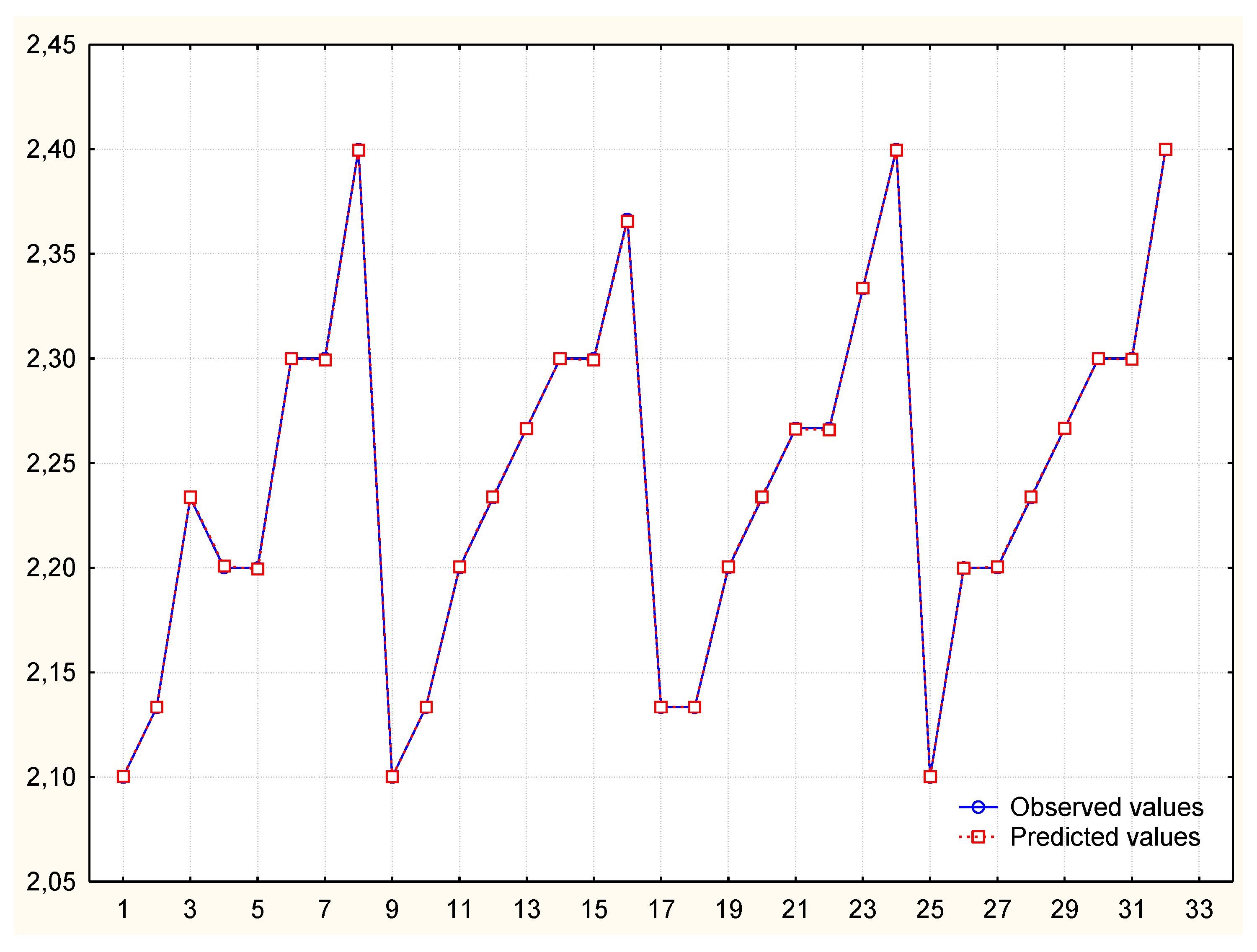
Based on the calculations and analysis of their results (Figure 17, Figure 18 and Figure 19), the correctness of the adopted model is confirmed.

4. Discussion

Five main directions of scheduling development can be distinguished: the first including the introduction of fuzzy data [22,23], the second taking into account time buffers [24,25], the third introducing risk factors [26], the fourth regarding task scheduling using artificial intelligence tools [27,28], and the fifth involving pipeline task scheduling [29]. A common feature of all faculties is the use of work input values as an element necessary to create a schedule. In construction, the amount of work [30] is given in the form of the total work time of all workers performing a specific task. Establishing the input standard is difficult because the input for the same production unit is not always the same. They depend on many factors, such as: method of construction and type of construction, type and grade of materials used, qualifications and abilities of workers, working conditions, technique and technology of execution, quality requirements, number of works to be performed, and size of the working team. The expenditure standards obtained in this way are averaged values and may significantly differ from the time the work was carried out under certain conditions.
The use of average time for employees in the schedule is different from the actual values for individual employees and may be the reason for non-compliance. The methodology presented in the article is more accurate and allows better estimation of the time needed to complete a given number of elements by an employee.
After conducting a number of analyzes using various calculation methods, it is possible to assess their usefulness in the employee performance forecast. Analyzing the collected data manually, it could be seen that there is a relationship between the independent variables “employee experience” and “number of elements made” and the dependent variable “employee performance”. In practice, it is often found that employee performance depends on their seniority in similar positions. Correlation analysis only confirmed the authors’ suppositions. It was necessary to exclude one of the correlated independent variables in order to improve the prediction model of some methods (as in the MR1 method).
The results of individual analyzes are summarized in the table below (Table 13).
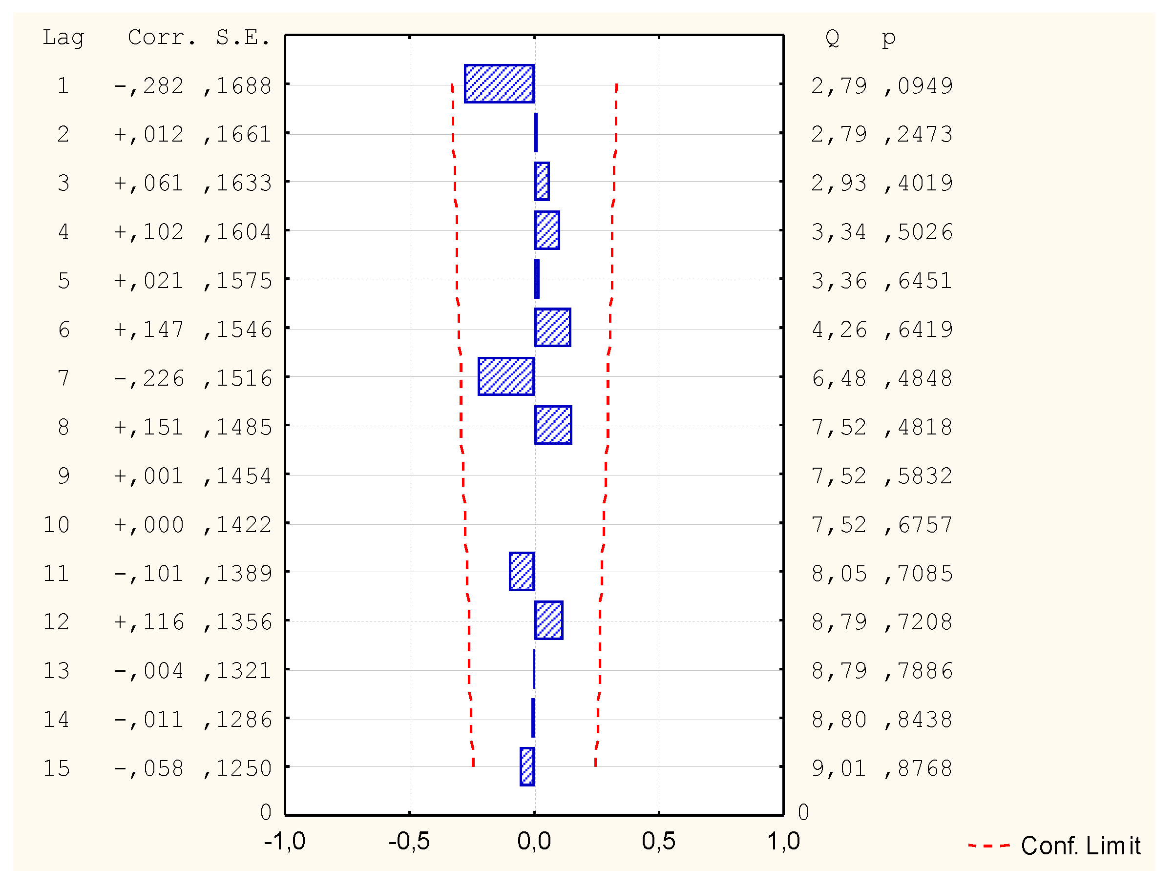
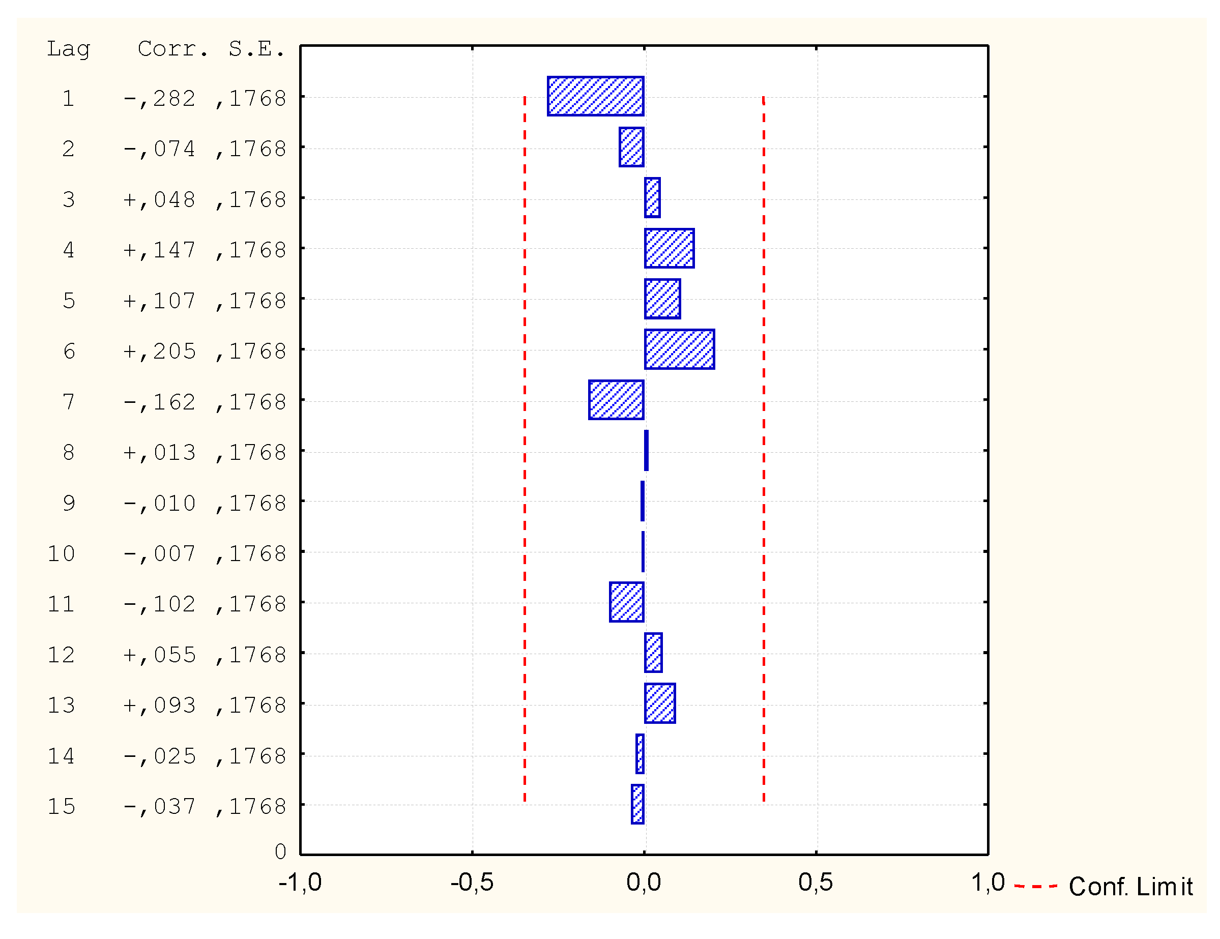
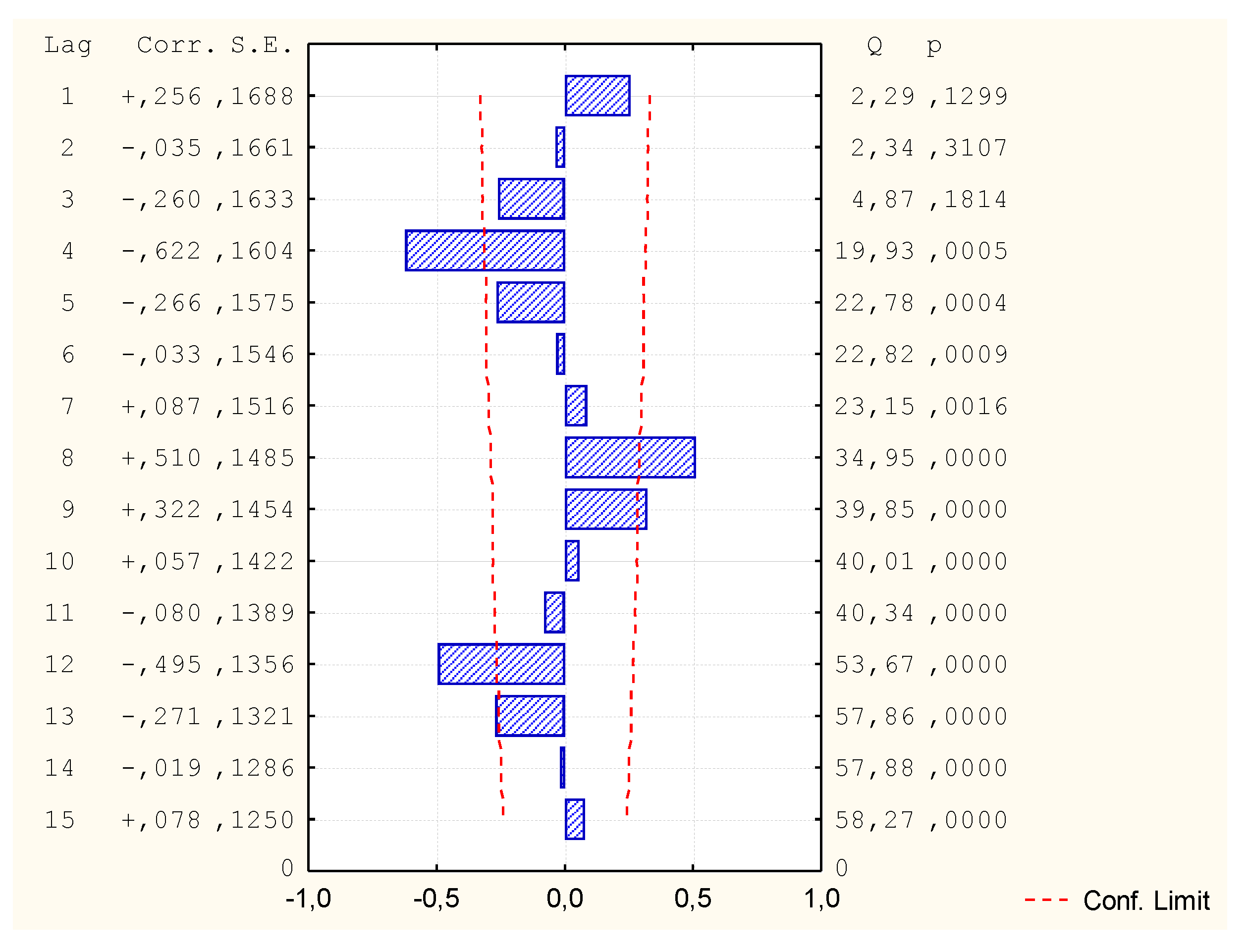
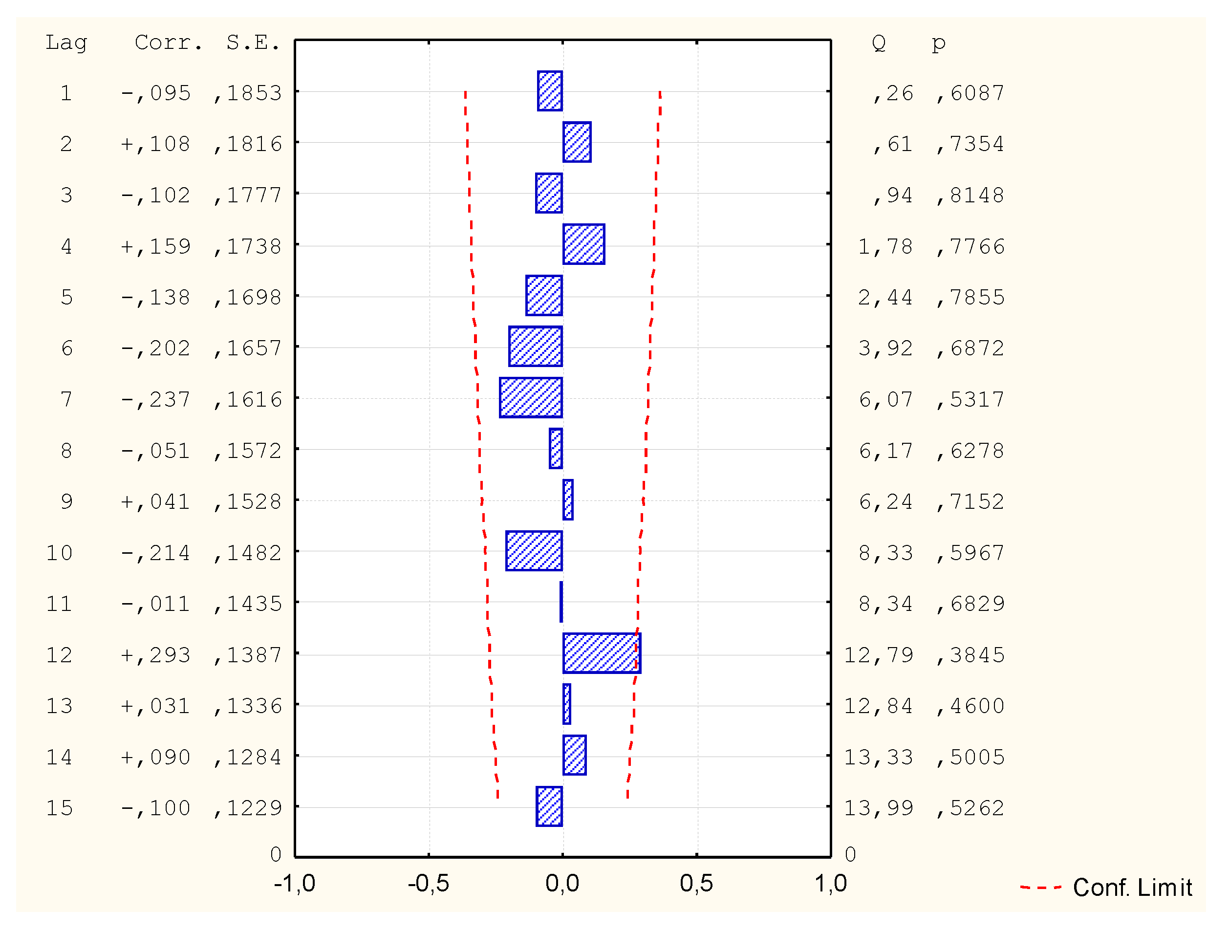
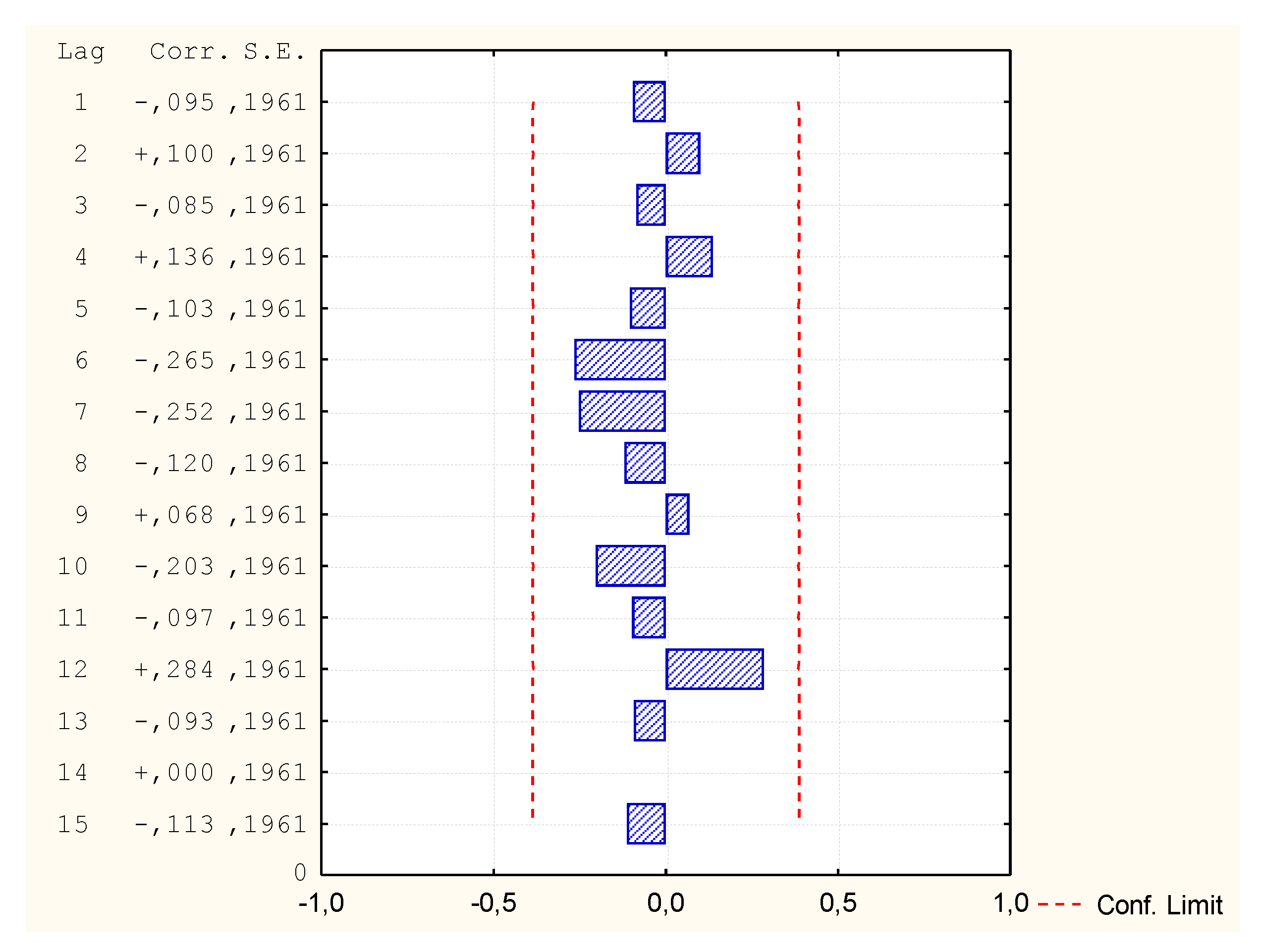
The correctness of calculations was determined based on the function of residue correlation and partial autocorrelation of residues. The residual series, which arises as the difference between the measured values and the predicted values, should have an average close to zero. At the same time, its standard deviation need not be zero. If the model is correct, no random correlation should occur. However, computational practice shows that if the limit values are not exceeded in the first 8 delays, the model can be assumed to be correct.
All examined residual autocorrelation and partial residual autocorrelation plots were summarized for 15 delays and their limits. Table 13 shows that several methods exceeded limit values in the first 8 delays. Therefore, it should be stated that the hypothesis about the presence of residues in these cases was confirmed and the equation from which the residual series can not be a regression equation. Based on residue autocorrelation and partial residue autocorrelation, MR2, GAM1, and GAM2 models were rejected. Other models meet the criterion.
Of the many available measures for assessing the accuracy of prediction and calculation of errors, it was decided to use the MAPE error, because it is the most reliable. This is the basic measure of the correctness of calculations. In the assessment of the forecast, the criterion was adopted in which the MAPE error below 1% is considered to be highly accurate, from 1–3% as good, and above 3% as not good.
The MAPE error calculations were made only for the correct models and all forecasts can be considered highly accurate because their error value is less than 1%. The best prediction was obtained by the method of automatic neural networks and amounts to 0.02%.

5. Conclusions

The presented work shows various computational models of the MMSM method, thanks to which it is possible to predict employees’ work performance quickly and accurately. At present, anticipating employee performance and the length of time they work, or the time it takes to perform a specific task, is time consuming and often complicated. The methodology presented in the article is possible to apply in various sectors of the economy. Any company with input data that wants to gain better control and predict the plant’s performance can use the presented methodology. Based on the research conducted, the following conclusions were made:
(1)
Forecasting and prediction is possible based on the regression formula of employee performance by the MMSM method. The method shows how certain characteristic variables for this process have an impact on the duration of works;
(2)
Half of the analyzed models is correct and reflects employee performance very accurately. It is possible to use selected models to assess employee performance and the duration of work for a specific order;
(3)
The best forecast was obtained using the automatic neural network method, MAPE = 0.02%. The disadvantage of this method is the lack of a regression pattern, which limits its universality. New calculations can be made by a person who has all previous data and a neural network.
The research will be continued in the context of the specialization of the work of individual employees. Division of employees into sections performing permanent and simple tasks, thanks to which it will be possible to increase employee productivity and thus increase the efficiency of the entire plant. It is planned to collect further data, in a similar way as shown in the work. Then the plant will be reorganized. Employees will not perform the entire item from beginning to end as it has been until now. Complex elements will be divided into simple and repeatable sections. Each employee will be assigned to perform a repetitive operation. The collected data will be compared. It is possible that the next work will bring new solutions.

Author Contributions

Conceptualization, P.K.-D. and M.R.; Methodology, M.R. and P.K.-D.; Software, P.K.-D.; Validation, M.R. and P.K.-D.; Formal Analysis, P.K.-D.; Investigation, P.K.-D.; Resources, M.R. and P.K.-D.; Data Curation, M.R. and P.K.-D.; Writing-Original Draft Preparation, P.K.-D.; Writing-Review & Editing, M.R. and P.K.-D.; Visualization, P.K.-D.; Supervision, M.R.; Project Administration, P.K.-D.; Funding Acquisition, M.R. and P.K.-D. All authors have read and agreed to the published version of the manuscript.

Funding

This research received no external funding.

Conflicts of Interest

The authors declare no conflict of interest.

Signs

MMSMMultivariate Method of Statistical Models
MRMultiple Regresion
MARSMultivariate Adaptive Regression Splines
GAMGeneralized Additive Models
NNNeural Networks
MAPEMean Absolute Percentage Error

References

  1. Paprocka, I. The model of maintenance planning and production scheduling for maximising robustness. Int. J. Prod. Res. 2019, 57, 4480–4501. [Google Scholar] [CrossRef]
  2. Plebankiewicz, E.; Juszczyk, M.; Malara, J. Estimation of task completion times with the use of the pert method on the example of a real construction project. Arch. Civ. Eng. 2015, 61, 51–62. [Google Scholar] [CrossRef]
  3. Sawicki, M.; Szostak, M.; Beben, D.; Rak, A.; Perkowski, Z. Analysis of the Dependence between the Number of Accidents at Workplaces that Involve Scaffolding and Changes in Work Efficiency. In Proceedings of the 3rd Scientific Conference Environmental Challenges in Civil Engineering (ECCE 2018), Opole, Poland, 23–25 April 2018; Volume 174. [Google Scholar]
  4. Beck, J.; Shen, W. The Effects of US Presidential Elections on Work Engagement and Job Performance. Appl. Psychol. Int. Rev. Psychol. Appl. Rev. Int. 2019, 68, 547–576. [Google Scholar] [CrossRef] [Green Version]
  5. Kuprenas, J.; Ghafoori, N. Influence of Construction Costs on Schedule Performance. In Challenges, Opportunities and Solutions in Structural Engineering and Construction; CRC Press: Boca Raton, FL, USA, 2010; pp. 903–905. [Google Scholar]
  6. Hasan, M.; Qayyum, Z.; Hasan, S. Planning and Scheduling of Manpower in an Annualized Hours Environment Integrating Workers Willingness and Efficiency. Ind. Eng. Manag. Syst. 2019, 18, 1–24. [Google Scholar] [CrossRef]
  7. Li, K.; Xu, S.; Fu, H. Work-break scheduling with real-time fatigue effect and recovery. Int. J. Prod. Res. 2019, 58. [Google Scholar] [CrossRef]
  8. Tucker, P. The impact of rest breaks upon accident risk, fatigue and performance: A review. Work Stress 2003, 17, 123–137. [Google Scholar] [CrossRef]
  9. Pahos, N.; Galanaki, E. Staffing Practices and Employee Performance: The Role of Age. In Evidence-Based HRM: A Global Forum for Empirical Scholarship; Emerald Publishing Limited: Bingley, UK, 2019; Volume 7, pp. 93–112. [Google Scholar]
  10. Aliekperova, N. Motivating factors effecting work efficiency of empoyees in ukrainian pharmaceutical sector. Econ. Sociol. 2018, 11, 61–74. [Google Scholar] [CrossRef] [PubMed] [Green Version]
  11. Khalil, F. Sexual frustration, religiously forbidden actions and work efficiency-a case study from the Pakistan perspective. Contemp. Islam-Dyn. Muslim Life 2016, 10, 477–487. [Google Scholar] [CrossRef]
  12. Rogalska, M. Multifactorial Models in Forecasting the Time of Construction Processes; Lublin Technical University: Lublin, Poland, 2016. [Google Scholar]
  13. Krzysztofiak, M.; Luszniewicz, A. Statistics; PWE: Warszawa, Poland, 1976. [Google Scholar]
  14. Shapiro, S.S.; Wilk, M.B. An analysis of variance test for normality (complete samples). Biometrika 1965, 52, 591–611. [Google Scholar] [CrossRef]
  15. Navarra, A.; Simoncini, V.; Navarra, A.; Simoncini, V. Multiple Linear Regression Methods. In Guide to Empirical Orthogonal Functions for Climate Data Analysis; Springer: New York, NY, USA, 2010; pp. 123–146. [Google Scholar]
  16. Rogalska, M. Forecasting the Duration of Failure of Wheeled Excavators Using the Methods of Neural Networks, Multiple Regression and ARIMA; Lublin Technical University: Lublin, Poland, 2012. [Google Scholar]
  17. Giudici, P. Applied Data Mining. Statistical Methods for Business and Industry; John Wiley & Sons Ltd.: Chichester, UK, 2003. [Google Scholar]
  18. Friedman, J.; Hastie, T.; Tibshirami, R. The Elements of Statistical Learning. Data Mining, Inference, and Prediction, 2nd ed.; Springer: Berlin/Heidelberg, Germany, 2016. [Google Scholar]
  19. Hastie, T.; Tibshirani, R. Generalized Additive-Models—Some Applications. J. Am. Stat. Assoc. 1987, 82, 371–386. [Google Scholar] [CrossRef]
  20. Hestie, T.J.; Tibshirani, R.J. Generalized Additive Models; Chapman Hall: London, UK, 1990. [Google Scholar]
  21. De Myttenaere, A.; Golden, B.; Le Grand, B.; Rossi, F. Mean Absolute Percentage Error for regression models. Neurocomputing 2016, 192, 38–48. [Google Scholar] [CrossRef] [Green Version]
  22. Chanas, S.; Zieliński, P. Critical Path Analysis in the Network with Fuzzy Activity Times. Fuzzy Sets Syst. 2001, 122, 195–204. [Google Scholar] [CrossRef]
  23. Chen, S.P. Analysis of Critical Paths in Project Network with Fuzzy Activity Times. Eur. J. Oper. Res. 2007, 183, 442–459. [Google Scholar] [CrossRef]
  24. Rogalska, M.; Hejducki, Z. Time buffers in construction process scheduling. J. Civ. Eng. Manag. 2007, 13, 143–148. [Google Scholar] [CrossRef]
  25. Steyn, H. Project management applications of the theory of constraints beyond critical chain scheduling. Int. J. Proj. Manag. 2002, 20, 75–80. [Google Scholar] [CrossRef]
  26. Li, C.; Wang, K. The risk element transmission theory research of multi-objective risk-time-cost trade-off. Comput. Math. Appl. 2009, 57, 1792–1799. [Google Scholar] [CrossRef] [Green Version]
  27. Prakash, A.; Felix, T.S.; Chan, F.T.S.; Deshmukh, S.G. FMS scheduling with knowledge based genetic algorithm approach. Expert Syst. Appl. 2011, 38, 3161–3171. [Google Scholar] [CrossRef]
  28. Nassar, K. Evolutionary optimization of resource allocation in repetitive construction schedules. J. Inf. Technol. Constr. 2005, 10, 265. [Google Scholar]
  29. Rogalska, M.; Hejducki, Z. Shortening the realisation time of building project with application of theory of constraints and critical chain scheduling. J. Civ. Eng. Manag. 2004, 10, 99–105. [Google Scholar]
  30. Kowalczyk, Z.; Zabielski, J. Cost Estimation and Standardization in Construction; WSiP: Warszawa, Poland, 2012. [Google Scholar]
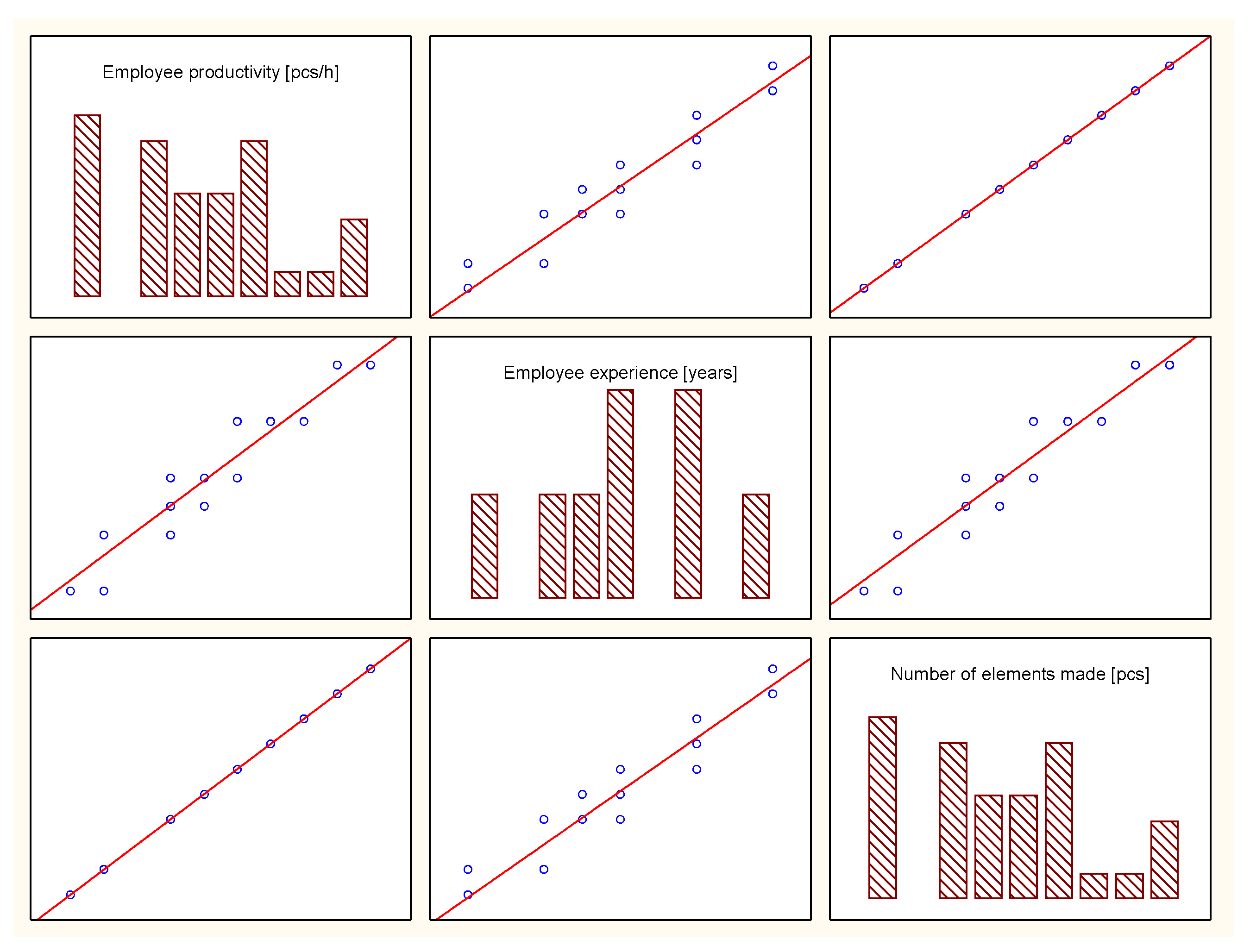
Figure 1. Correlation between employee productivity, employee experience and number of elements made.
Symmetry 12 00413 g001
Figure 2. Comparison of observed values and predictions.
Symmetry 12 00413 g002
Figure 3. Autocorrelation function—rest.
Symmetry 12 00413 g003
Figure 4. Partial autocorrelation function—rest.
Symmetry 12 00413 g004
Figure 5. Comparison of observed values and predictions.
Symmetry 12 00413 g005
Figure 6. Autocorrelation function—rest.
Symmetry 12 00413 g006
Figure 7. Partial autocorrelation function—rest.
Symmetry 12 00413 g007
Figure 8. Comparison of observed values and predictions.
Symmetry 12 00413 g008
Figure 9. Autocorrelation function—rest.
Symmetry 12 00413 g009
Figure 10. Partial autocorrelation function—rest.
Symmetry 12 00413 g010
Figure 11. Comparison of observed values and predictions.
Symmetry 12 00413 g011
Figure 12. Autocorrelation function—rest.
Symmetry 12 00413 g012
Figure 13. Partial autocorrelation function—rest.
Symmetry 12 00413 g013
Figure 14. Comparison of observed values and predictions.
Symmetry 12 00413 g014
Figure 15. Autocorrelation function—rest.
Symmetry 12 00413 g015
Figure 16. Partial autocorrelation function—rest.
Symmetry 12 00413 g016
Figure 17. Comparison of observed values and predictions.
Symmetry 12 00413 g017
Figure 18. Autocorrelation function—rest.
Symmetry 12 00413 g018
Figure 19. Partial autocorrelation function—rest.
Symmetry 12 00413 g019
Table 1. Measurements of employee performance and independent variables affecting it.
Employee Productivity [pcs/h]Employee Experience [years]Number of Elements Made [pcs]Failure/Equipment Repair [%]Temp. [°C]Grinding Time [h]Well-Being Assessment [1–5]
Day 12.10115.753.52143
2.13316.003213.253
2.23416.7552134
2.20516.504.5213.254
2.20516.505.52135
2.30717.254213.253
2.30717.254.3213.253
2.40918.004.3213.255
Day 22.10115.753.521.53.54
2.13316.00321.53.754
2.20416.50521.534
2.23516.754.521.53.253
2.27517.005.521.534
2.30717.25421.53.253
2.30717.254.321.53.254
2.37917.754.321.52.753
Day 32.13116.003.520.53.254
2.13316.00320.53.753
2.20416.50520.53.52
2.23516.754.520.53.253
2.27517.005.520,53.254
2.27717.00420.532
2.33717.504.320.52.753
2.40918.004.320.534
Day 42.10115.753.5213.53
2.20316.503213.54
2.20416.5052133
2.23516.754.5213.253
2.27517.005.5212.754
2.30717.254213.253
2.30717.254.3212.754
2.40918.004.3212.53
Table 2. Results of the distribution normality test.
No.Variable NameChartW
v1Employee productivity [pcs/h] Symmetry 12 00413 i0010.948
v2Employee experience [years] Symmetry 12 00413 i0020.930
v3Number of elements made [pcs] Symmetry 12 00413 i0030.948
v4Failure/equipment repair [%] Symmetry 12 00413 i0040.933
v5Temp. [°C] Symmetry 12 00413 i0050.810
v6Grinding time [h] Symmetry 12 00413 i0060.938
v7Well-being assessment Symmetry 12 00413 i0070.839
Table 3. Summary of the correlation study.
VariableCorrelations Marked Correlations are Significant at p < 0.05000
N = 32 (Casewise Deletion of Missing Data) CumulativePe
MeansStd.Dev.Employee Productivity [pcs/h]Employee Experience [years]Number of Elements Made [pcs]Failure/Equipment Repair [%]Temp. [℃]Grinding Time [h]Well-Being Assessment [1–5]
Employee productivity [pcs/h]2.2420.0881.0000.9651.0000.379−0.034−0.6760.055
Employee experience [years]5.1252.4060.9651.0000.9650.3240.000−0.636−0.016
Number of elements made [pcs]16.8130.6601.0000.9651.0000.379−0.034−0.6760.055
Failure/equipment repair [%]4.2630.7520.3790.3240.3791.0000.000−0.5550.213
Temp. [°C]21.0000.359−0.0340.000−0.0340.0001.0000.0000.250
Grinding time [h]3.1950.322−0.676−0.636−0.676−0.5550.0001.000−0.095
Well-being assessment [1–5]3.4690.7180.055−0.0160.0550.2130.250−0.0951.000
Table 4. Summary of multiple regression results MR1 (v1; v2, v5, v6, v7).
MR1 (v1; v2, v5, v6, v7)
Dependent Variable: v1; Independent Variable: v2, v5, v6, v7
N = 32Regression Summary for Dependent Variable: Employee Productivity [pcs/h]
R = 0.97151969 R2 = 0.94385051 Adjusted R2 = 0.93553207
F(4.27) = 113.46 p < 0.00000 Std.Error of estimate: 0.02234
BetaStd. Err. of BetaBStd. Err. of Bt (27)p-Level
Intercept 2.3903920.2441509.790670.000000
v20.9082200.0594070.0332100.00217215.288030.000000
v6−0.0910910.059686−0.0248810.016303−1.526170.138598
v70.0747360.0475820.0091620.0058331.570670.127906
v5−0.0527230.047132−0.0129140.011545−1.118630.273151
Regression formula: v1 = 2.390392 + 0.033210v2 – 0.024881v6 + 0.009162v7 – 0.012914v5.
Table 5. Summary of multiple regression results MR2 (v1; Log(v3), v4, v7).
MR2 (v1; Log(v3), v4, v7)
Dependent Variable: v1; Independent Variable: Log(v3), v4, v7
N = 32Regression Summary for Dependent Variable: Employee Productivity [pcs/h]
R = 0.99984602 R2 = 0.99969206 Adjusted R2 = 0.99965907
F(3.28) = 30300, p < 0.0000 Std.Error of Estimate: 0.00162
BetaStd. Err. of BetaBStd. Err. of Bt (27)p-Level
Intercept −4.110470.022218−185.0090.000000
Log(v3)1.0047220.0036022.253070.008078278.9090.000000
v4−0.0133750.003682−0.001570.000431−3.6330.001114
v70.0048190.0033960.000590.0004161.4190.166949
Regression formula: v1 = −4.11047 + 2.25307Log(v3) – 0.00157v4 + 0.00059v7.
Table 6. Model specifications of MARSplines method.
Model SpecificationsModel Summary
Value
Independents5
Dependents1
Number of terms2
Number of basis functions1
Order of interactions1
Penalty2.000000
Threshold0.000500
GCV error0.000629
PruneYes
Table 7. Number of times each predictor is used in MARSplines method.
DependentsNumber of References to Each Predictor
Number of Times Each Predictor is Referenced (Used)
References
Employee experience [years]1
Failure/equipment repair [%]0
Temperature [°C]0
Grinding time [h]0
Well-being assessment [1–5]0
Table 8. Model coefficients, knots and basis functions of MARSplines method.
Coefficients, Knots and Basis FunctionsModel Coefficients
NOTE: Highlighted Cells Indicate Basis Functions of Type
Max(0, Independent-Knot), otherwise Max(0, Knot-Independent)
Coefficients v1Knots v2Knots v3Knots v4Knots v5Knots v6Knots v7
Intercept2.096123------
Term.10.0352831.00-----
Regression formula: v1 = 2.09612349117920 + 0.0352831940575674 * max(0; v2 −1.0000000000000)
Table 9. Summary of GAM method.
Variable IndexDegrees of FreedomGAM CoefficientStd. Err.Result Std.p-Level
Intercept01.000000−0.0203110.012648−1.6058
v213.999711−0.0008970.000204−4.39320.000000
v323.9984110.1348330.000779173.14060.000000
v434.0013880.0000790.0002060.38230.000000
v644.000114−0.0001980.000595−0.33290.933869
Regression formula: v1 = −0.020311 − 0.000897v2 + 0.134833v3 + 0.000079v4 − 0.000198v6.
Table 10. Model specifications of GAM2 method.
Variable IndexDegrees of FreedomGAM CoefficientStd. Err.Result Std.p-Level
Intercept01.000000−0.1933600.001631−118.549
v213.999711−0.0000190.000026−0.7030.000000
v323.9984110.0595000.000100592.4870.000000
v434.001388−0.0000240.000027−0.9190.948296
v644.000114−0.0000960.000077−1.2550.580771
Regression formula: v1 = e^(−0.193360 – 0.000019v2 + 0.059500v3 – 0.000024v4 – 0.000096v6).
Table 11. Information about perf. and error value of NN method.
IndexNet. NameTraining Perf.Test Perf.Training ErrorTest Error
1MLP 6-7-10.9999850.9999910.0000020.000002
Table 12. Information.
Training AlgorithmError FunctionHidden ActivationOutput Activation
BFGS 17SOSTanhIdentity
Table 13. Summary of calculations carried out by selected methods.
Method NameAutocorrelation of Residues or Partial ResiduesModel CorrectnessMAPE Error [%]
MR1 (v1; v2, v5, v6, v7)Does not occurCorrect0.72
MR2 (v1; Log(v3), v4, v7)In 6th placeIncorrect-
MARS1 (v1; v2, v4, v5, v6, v7)Does not occurCorrect0.82
GAM1 (v1; v2, v3, v4, v6In 4th placeIncorrect-
GAM2 (v1; v2, v3, v4, v5, v6, v7)In 8th placeIncorrect-
NN1 (v1; v2, v3, v4, v5, v6, v7)In 12th placeCorrect0.02