Automated Sustainable Multi-Object Segmentation and Recognition via Modified Sampling Consensus and Kernel Sliding Perceptron

Abstract

Object recognition in depth images is challenging and persistent task in machine vision, robotics, and automation of sustainability. Object recognition tasks are a challenging part of various multimedia technologies for video surveillance, human–computer interaction, robotic navigation, drone targeting, tourist guidance, and medical diagnostics. However, the symmetry that exists in real-world objects plays a significant role in perception and recognition of objects in both humans and machines. With advances in depth sensor technology, numerous researchers have recently proposed RGB-D object recognition techniques. In this paper, we introduce a sustainable object recognition framework that is consistent despite any change in the environment, and can recognize and analyze RGB-D objects in complex indoor scenarios. Firstly, after acquiring a depth image, the point cloud and the depth maps are extracted to obtain the planes. Then, the plane fitting model and the proposed modified maximum likelihood estimation sampling consensus (MMLESAC) are applied as a segmentation process. Then, depth kernel descriptors (DKDES) over segmented objects are computed for single and multiple object scenarios separately. These DKDES are subsequently carried forward to isometric mapping (IsoMap) for feature space reduction. Finally, the reduced feature vector is forwarded to a kernel sliding perceptron (KSP) for the recognition of objects. Three datasets are used to evaluate four different experiments by employing a cross-validation scheme to validate the proposed model. The experimental results over RGB-D object, RGB-D scene, and NYUDv1 datasets demonstrate overall accuracies of 92.2%, 88.5%, and 90.5% respectively. These results outperform existing state-of-the-art methods and verify the suitability of the method.

1. Introduction

Human beings are capable of perceiving and recognizing multiple objects in complex scenarios via biological vision. Designing machines that are sufficiently intelligent to recognize and classify objects in complicated scenes has been a decades-long, intense area of research. However, recognition and classification are now significantly more precise and accurate due to the emergence of intelligent visualization by machines and robotics [1,2]. Object recognition is divided into two classes: 2D images and 3D point-clouds. By projecting the scene onto a plane, 2D images are generated by recording the light intensity measured at each point. In addition, 3D point-clouds map points in the scene from 3D coordinates. The only disparity between 2D and 3D is knowledge of depth, which is purely a component of 3D data. To represent the 3D information from the real world, inexpensive devices (sensors) such as Microsoft Kinect have been devised and used to capture depth information correlated with each pixel coupled with the Red-Green-Blue (RGB) image.

In addition, researchers have achieved significant developments in computer vision for sustainability in recent decades, with distinct outcomes for object detection and recognition. Fortunately, numerous methods perform relatively well at classifying only prominent objects in a complete scene; however the results are not adequate when multiple objects need to be recognized in a single dynamic scenario. In these methods, different features of objects, such as global and local features, are used to recognize objects in the scene. These scenes are comprised of multiple evident cues, including color, light intensities, corners, edges, point clouds, and templates, which can help recognize and analyze objects in complex scenes. In various applications, object segmentation and recognition are now increasingly being adopted in sustainable frameworks, such as visual tracking, medical diagnostics, scene understanding, and environmental monitoring. However, multiple objects are often coupled together in several scenes depicting their mutual relationships and inconsistencies across scenes, rendering scene recognition a perplexing task in visual analysis.

To deal with limitations in object recognition, we propose a sustainable multi-object recognition system that retains its efficiency despite any transition in the nature of the object or the scene. The system is based on modified maximum likelihood estimation sampling consensus, depth kernel descriptors (DKDES), and a kernel sliding perceptron (KSP). The proposed system performs pre-processing of the images as a first step. The pre-processed images are converted to point clouds and depth maps to extract planes for efficient segmentation using modified maximum likelihood estimation sampling consensus (MMLESAC) in the second step. As a third step, DKDES are computed over segmented objects. The computed DKDES are then forwarded to IsoMap for the selection and reduction of suitable features. The reduced DKDES set is then provided to a KSP for sustainable object recognition as a final step. Our contributions are as follows:

• Modified maximum likelihood estimation sampling consensus is proposed for the segmentation of depth objects.
• To reduce the dimensions of feature sets, and for better accuracy and efficiency, Isometric Mapping (IsoMap) is used.
• To recognize single and multiple objects in an image, a collective set of descriptors named depth kernel descriptors (DKDES) is applied to three benchmark datasets.
• To the best of our knowledge, the integrated KSP multi-depth kernel descriptor for identification of multiple objects is originally introduced here.
• To evaluate the reliability and consistency of the proposed system, a comprehensive statistical study is performed and compared with the latest methods.

Related work is summarized in Section 2. Section 3 offers a vision of the methodology including the proposed framework for object recognition. Experimental analysis of datasets, with an overview of these datasets, is given in Section 4. Finally, the conclusion and future work is presented in Section 5.

2. Related Work

Various studies have progressively employed different object recognition strategies in recent decades. Although object detection is a challenging task in sustainable visual recognition, scene understanding, and robotics, several researchers have devoted their efforts to the field. We reviewed literature in various fields, such as sustainable multi-object segmentation, image recognition, labeling, and recognition of objects in RGB, in addition to depth images, to appropriately analyze and evaluate our proposed system.

2.1. Sustainable Multi-Objects Segmentation via RGB Images

Image segmentation is aimed at clustering pixels into vital image fragments, i.e., fragments that correspond to particular structures, artifacts, or normal fragments of objects [3]. Image segmentation is a mid-level processing technique used to analyze images. This technique groups the pixels to form homogeneous regions based on pixel characteristics, such as color, texture, intensity, and other characteristics, to classify or cluster the image into different and distinct fragments [4,5]. The key task of the segmentation process is to specifically distinguish the object in the scene from the background.

Numerous researchers [6,7] have considered color spaces as important cues for color image segmentation. Jurio et al. [8] compared multiple color spaces using cluster-based segmentation to focus on similar techniques. They included four color spaces: HSV (Hue, Saturation and Value), CMY (Cyan, Magenta and Yellow), RGB, and YUV to determine the best color representation model. Although HSV produced good results, they achieved the highest accuracy with the CMY color model. A. K. Sinop et al. [9] describes their graph-cut algorithm for image segmentation separating the foreground object form the background. The technique considers the whole image with its morphological details for efficient segmentation. P. Beunestado et al. [3] proposed an image segmentation method that combines the statistical confidence interval with the standard Otsu technique to achieve improved segmentation results. They enhanced the image using their proposed method using a statistical confidence interval and then applied the Otsu algorithm, which provided good results compared to the standard Otsu algorithm.

2.2. Sustainable Multi-Object Recognition via RGB Images

Multi-object recognition is more complicated because one image consists of several instances with a cluttered environment and complicated backgrounds in various locations. M. Rashid et al. [10] used a deep learning architecture based on multi-layer deep feature selection and fusion for object recognition. Their approach yielded accurate recognition results using three steps, including two deep learning architecture elements, i.e., for the fusion of features, a deep convolution network for image recognition, and Inspection V3 for feature extraction. Additionally, they molded parallel maximum covariance, and for the selection of best features, a logistic regression controlled the entropy variance algorithm. A. Ahmed et al. [11] used multiple algorithms in a pipeline for multiple object recognition over an RGB dataset. They extracted similar regions over an image via a k-means clustering algorithm and achieved segmentation by merging similar regions. They considered the generalized Hough transform (GHT) algorithm for object detection and a genetic algorithm as an object recognizer. S. Zia et al. [12] suggested a solution for object recognition using a deep convolutional neural network (CNN). They designed a hybrid 2D/3D CNN that used a pretrained network. Furthermore, they trained their CNN over a small RGB-Depth dataset. They combined the features extracted from both RGB-only and depth-only models, in their hybrid model, to produce more accurate results. A. Ahmed et al. [13] proposed a novel method to recognize multi-objects in a scene based on object categorization. They segmented the image by employing improved fuzzy c-mean and mean shift segmentation techniques. Subsequently, local descriptors are extracted and multiple kernel learning is applied for object categorization. Additionally, they incorporated intersection over union scores and multi-class logistic regression for scene classification.

2.3. Sustainable Multi-Object Segmentation via Depth Images

Segmenting an image into several regions is known as depth segmentation. In recent decades, depth data has been used to achieve enhanced performance. Some researchers consider color, depth, and combinations of both color and depth information to improve segmentation results, such as R. Xiaofeng et al. [14]. A new descriptor for object detection based on the histogram of oriented gradients (HOG) was proposed by D. Venkatrayappa et al. [15]. It combines HOG with an oriented response anisotropic derivative half Gaussian kernel. They ascertained the improved efficiency over scale-invariant feature transform (SIFT), gradient location and orientation histogram (GLOH), and DAISY descriptors. To detect objects from depth images, a 3D detector was designed by S. Song et al. [16]. It considers complexities such as variations in texture, low illumination, cluttered or occluded objects, and different viewpoints during the object recognition process. Moreover, to obtain synthetic depth maps, they collected 3D CAD models to match multiple viewpoints. In addition, when extracting features from point clouds, they trained the exemplar support vector machine (SVM) model while a 3D detection window was used during testing in their proposed system. W. Shi et al. [17] introduced a multi-level cross-aware (MCA) model for the segmentation of indoor RGB-D images. MCA used depth geometric information, 2D appearance, and fused complementary features from RGB and depth images. They achieved remarkable results over the indoor RGB-D dataset.

2.4. Sustainable Multi-Objects Recognition via Depth Images

Multi-object recognition in depth images has numerous applications, such as image retrieval, autonomous vehicles, surveillance, and robotic navigation. U. Asif et al. [18] presented a hierarchical cascade forests model that uses computed probabilities at different phases of an image, based on which unknown objects and classes are recognized. They introduced an objective function that extracts features from the point clouds of RGB-D objects in the account of object recognition and grasp detection. A. Ahmed et al. [19] designed a novel technique to localize and recognize multiple objects in RGB-D indoor scenes. They used a fusion saliency map of objects and a centered darker channel for object segmentation, multiple feature descriptors, feature matching, and Hough voting for the recognition of multiple objects over the RGB-D dataset. L. Tang et al. [20] designed a convolution neural network framework based on canonical correlation analysis (CCA). They fused separately processed RGB and depth images through a CCA layer and a combining layer was introduced to the multi-view CNN. H. Liu et al. [21] developed an extreme learning machine (ELM) structure using a multi-modal local receptive field (MM-LRF). There, LRF is used as a feature extractor for each modality, and a shared layer is proposed for combining the features. Final objects are recognized through the ELM classifier. They achieved remarkable accuracy over single objects in a similar environment, but they did not consider either complex RGB-D images with multiple objects or different environments.

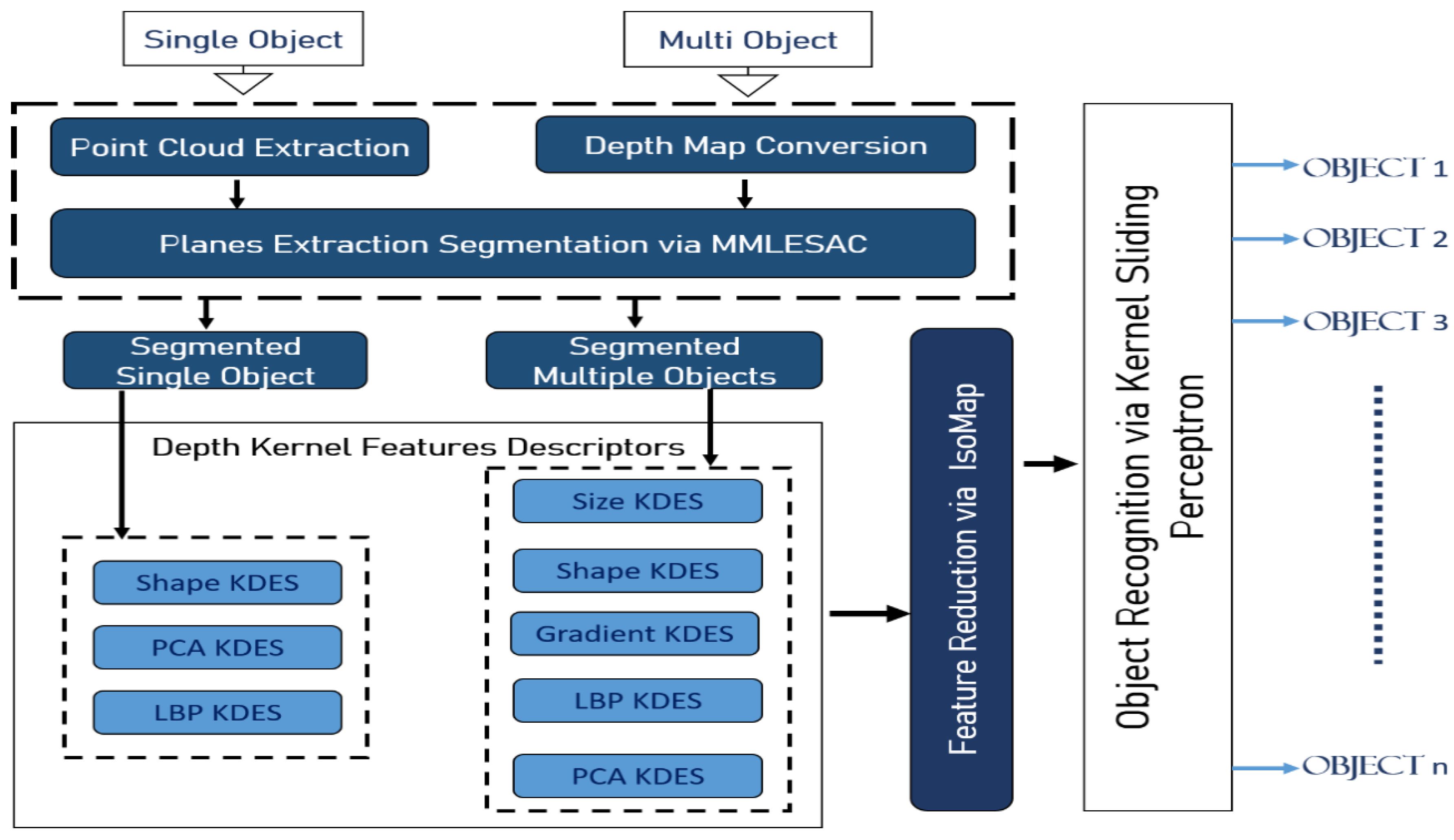
3. Proposed System Methodology

In this section, we propose a novel sustainable object recognition model that recognizes and labels multiple objects in depth images. Initially, a depth image is taken as input for point cloud extraction for a single object. For multiple object recognition, the depth image is converted to a depth map. After point cloud extraction or depth map conversion, plane fitting is applied using the proposed MMLESAC for object segmentation. Then, DKDES are computed over the segmented objects. The extracted depth descriptors are forwarded to IsoMap for feature reduction and selection. Finally, the reduced feature set is provided to a multi-layer KSP for object recognition. Figure 1 illustrates the overview of the proposed object recognition system using a KSP.

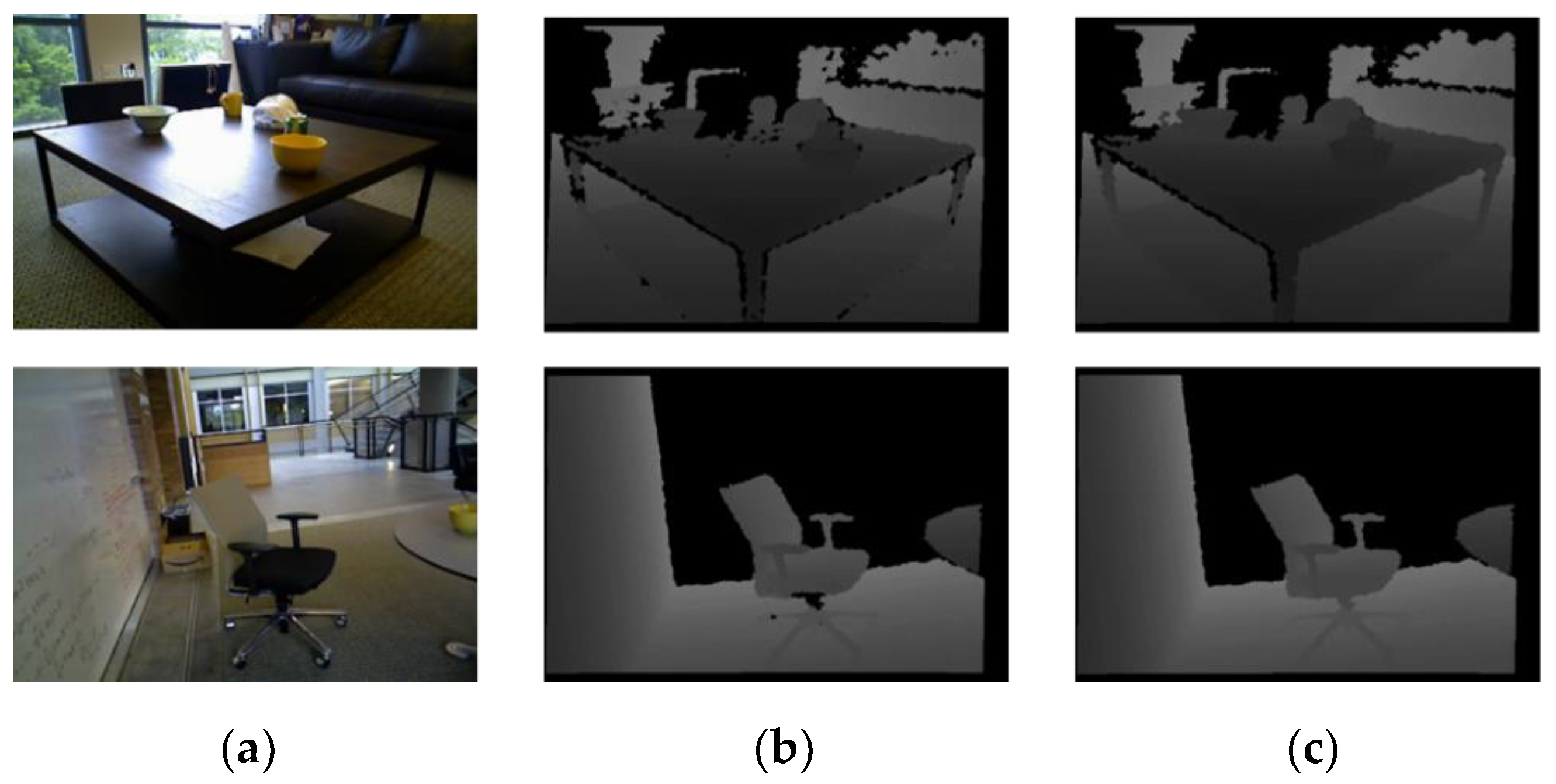
3.1. Image Acquisition and Preprocessing

During pre-processing, unwanted pixels that are caused due to various conditions, such as different illumination, thus, surrounding scenarios are removed (see Figure 2). To address these complications, filling of the holes is performed as a pre-processing step [22,23,24,25,26]. After filling, the image is smoothed using ideal low pass filters (ILPFs) by applying the following transfer function of the ILPF:

$$H\left(x,y\right)=\{\begin{array}{c}1 \mathrm{if}D\left(x,y\right)\le D_0\\ 0 \mathrm{if}D\left(x,y\right)>D_0\end{array}$$

(1)

$$D\left(x,y\right)={\left[{(x-M/2)}^2+{(y-N/2)}^2\right]}^{\raisebox{1ex}{$1$}\!\left/ \!\raisebox{-1ex}{$2$}\right.}$$

(2)

where $D\left(x,y\right)$ is the distance from point $\left(x,y\right)$ to the center of their pixels’ intensity rectangles. The filter using the ILPF removes the high intensity pixels and preserves the low intensity pixels, and has an intensity between 0 and 1, also known as the cutoff range.

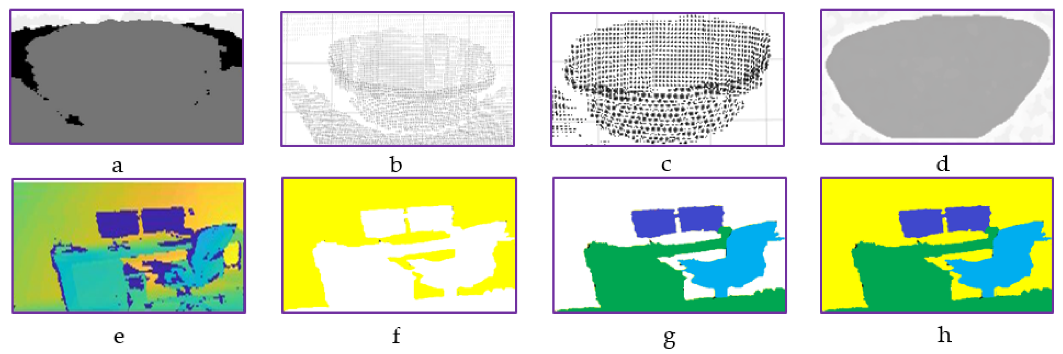
3.2. Objects Segmentation

In this section, a comprehensive description of single/multi-object segmentation is introduced. The purpose of segmenting an image is to partition it into appropriate small regions. These small regions or segments are more meaningful and understandable to a machine for further processing. As with most complex images, there are usually several regions and objects in complex scenes, thus, segmentation is a demanding yet critical process for accurate object recognition. Therefore, the quality of segmentation directly impacts the accuracy of object recognition. To improve the quality of segmentation, numerous researchers have adopted several different techniques for 2D and 3D object detection and recognition, such as edge based, region growing, model fitting, hybrid, and machine learning approaches. Model fitting, such as plane fitting [27] using MMLESAC, is proposed to process single/multi-object segmentation. Nevertheless, whereas the random sample consensus (RANSAC) algorithm evaluates eminence by counting the number of matches that ratify the current hypothesis, MLESAC checks the hypothesis’ probability by representing the distribution of errors as a mixture model.

3.2.1. Single-Object Segmentation Using Point Cloud

After refining the segmentation of RGB-D images, 3D point clouds [28] were devised with images for the different phases of module recognition, namely, feature extraction, feature matching, and object recognition. Losses in machine expenses can be substantially minimized. Figure 3 displays the RGB-D image’s cloud point visualization. The resampling of the nearest neighbor (NN) [29] is used to sample the point cloud to maximize the system’s computational cost because the point cloud is represented by the point pattern and its corresponding points. Resampling retains and does not change the original attributes of visuals. The general flow of point cloud segmentation is adopted as in [30]. Down sampling is achieved thus:

$$k\left(u\right)=\{\begin{array}{c}1; if \left|u\right|<0.5\\ 0; \mathrm{otherwise}\end{array}$$

(3)

3.2.2. Multi-Objects Segmentation Using MMLESAC

With the MMLESAC plane fitting technique, we improved depth segmentation over existing MLESAC and RANSAC methods. MLESAC [31,32,33,34] follows RANSAC’s [35,36,37,38,39,40] basic idea which produces hypothetical results based on consecutive marginal correspondence sets; in contrast, the other remaining correspondences are used to check the quality of the hypothesis. Although, based on the probabilistic approach, MLESAC evaluates via the random sampling hypothesis, it does not presume any such complexity in the earlier matching stage which is used to provide its data. Unlike other matching approaches, MLESAC is robust because it not only treats the same prior probability of being a mismatch, it also recognizes the uncertain possibility.

Maximum Likelihood Estimation (MLE)

To analyze an object’s location in the image/scene, following the idea of [41,42], the pose (viewpoint) estimation of an object is an intrinsic operation, which requires a set of features computed from that image/scene and can be written mathematically as:

$$\mathit{\theta }=i_{abc}\left(t\right)=T^{-1}{i}_{\alpha \beta \gamma }\left(t\right)=\left[\begin{array}{ccc}x& u& 1\\ y& v& 1\\ z& w& 1\end{array}\right]\left[\begin{array}{c}{i}_{\alpha }\left(t\right)\\ i_{\beta }\left(t\right)\\ i_{\gamma }\left(t\right)\end{array}\right]$$

(4)

where $\left(a,b,c\right)$ are known as translational components and $\left(\alpha ,\beta ,\gamma \right)$ are Euler angles. For object O with a set of features $\mathit{O}=\left\{{\mathit{O}}_{\mathbf{0}},{\mathit{O}}_{\mathbf{1}},{\mathit{O}}_{\mathbf{2}},\dots ,{\mathit{O}}_{\mathit{m}}\right\}$ in an image I with set of features $\mathit{I}=\left\{{\mathit{I}}_{\mathbf{0}},{\mathit{I}}_{\mathbf{1}},{\mathit{I}}_{\mathbf{2}},\dots ,{\mathit{I}}_{\mathit{m}}\right\}$, the likelihood of pose or viewpoint $\mathit{\theta }$ has a directly proportional relationship to the features $\mathit{I}$ in the image I.

$$L\left(\mathit{\theta }\mid \mathit{I}\right)\propto P\left(\mathit{I}\mid \mathit{\theta }\right)=\prod _{i=1}^N{f}_i\left({\mathit{I}}_i\mid \mathit{\theta }\right)$$

(5)

where $f_i\left({\mathit{I}}_i\mid \mathit{\theta }\right)$ is called the probability density function (PDF) that is responsible for observing and examining the viewpoint $\mathit{\theta }$ of the ith feature using a rotational and translational model. To approximate $\overline{ℱ}$, the fundamental matrix using MLE is applied such that:

$$\overline{ℱ}=\underset{\mathit{F}}{\overset{}{max}}\left\{\prod _{i=1}^n\mathfrak{p}\left({\epsilon }_i\mid ℱ\right)\right\}$$

(6)

where $\mathfrak{p}\left({\epsilon }_i\mid ℱ\right)$ is a likelihood function that describes how well the ith correspondence matches, when a fundamental matrix $ℱ$ is given. To quantify the correspondence match we used the $P(c_i)$ probability, which shows the probability of being correctly matched. We determined $P(c_i)$ using the similarity measure of the feature matcher, and each ith correspondence has different $P(c_i)$.

Modified Maximum Likelihood Estimation Sample Consensus (MMLESAC)

After determining the $P(c_i)$ of each correspondence, the error ${\epsilon }_i\left(ℱ\right)$ of the ith correspondence for each sample is calculated. We classified the whole correspondences of each sample into two sets, i.e., inliers and outliers, using a predefined threshold $T$ of error ${\epsilon }_i\left(ℱ\right)$ as follows:

$$\mathit{inlier}=\mathit{if}\Vert {\epsilon }_i\left(\mathit{F}\right)\Vert <T$$

(7)

$$\mathit{outlier},\mathit{if}\Vert {\epsilon }_i\left(\mathit{F}\right)\Vert \ge T$$

(8)

This classification outcome is used for the validity of the correspondences. Then, we achieved the estimation of $P(c_i)$ for the ith correspondence using the inlier–outlier classification (IOC) of the successful sample. Successful samples are those that have a better score than any previous sample. The IOC results for the ith correspondence at the nth successful random sample are $C_1^i, C_2^i,\dots ,C_n^i$ and the sum $S_n^i$ of all $n$ samples us given as:

$$S_n^i=C_1^i+C_2^i+\dots +C_n^i$$

(9)

Then, we estimated the correspondence validity using $S_n^i$ as:

$$P(c_i)\leftarrow \raisebox{1ex}{$S_n^i$}\!\left/ \!\raisebox{-1ex}{$n$}\right.$$

(10)

For initialization of the estimation, the values of $P(c_i)$ are assumed to be equal to 0.5 and a minimal subset $S_m$ of $k$ correspondences is selected randomly. Then, error ${\epsilon }_i\left(ℱ\right)$ is calculated for each correspondence and the scores of the hypotheses are determined using Equation (6). When a best hypothesis is determined, then IOC is applied to the whole dataset according to Equation (7) and Equation (8). Then the results are summed using Equation (9). The fraction $f$ and upper limit $up{p}_{max}$ are achieved using:

$$f=\frac{1}{j}\sum _{i=1}^j{C}_n^i$$

(11)

$$up{p}_{max}=\log \left(1-p\right)/\log \left(1-{(1-f)}^k\right)$$

(12)

The modified algorithm as defined above, is termed MMLESAC and explained here in Algorithm 1.

Algorithm 1. Modified Maximum Likelihood Estimation Sample Consensus (MMLESAC).

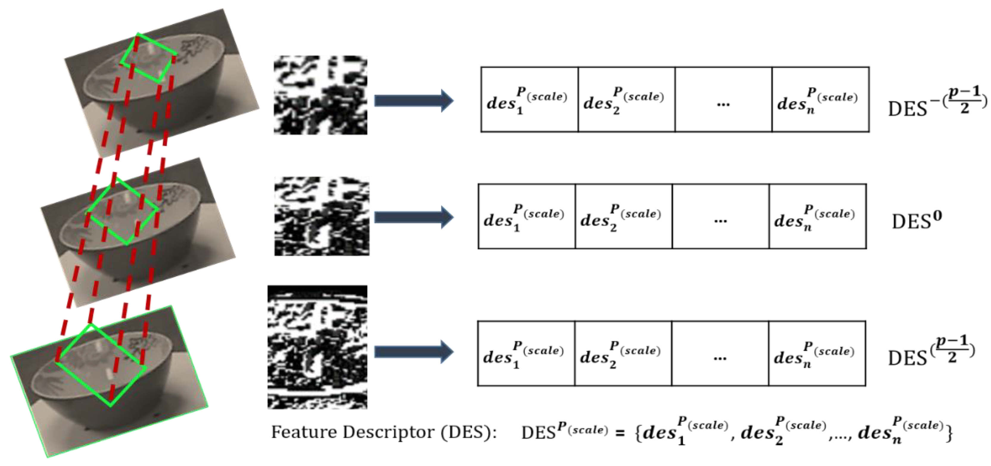
3.3. Feature Extraction via DKDES over Segmented Objects

To recognize the objects in the image, the pixel features [43,44,45,46,47,48] are computed in a small window around a single pixel. For instance, gradient location and orientation histogram (GLOH), a histogram of gradients (HOG), [49,50,51,52,53], and scale-invariant feature transform (SIFT) [54,55,56,57] are renowned techniques that compute pixel features, such as gradient magnitude and orientation. These techniques are based on histograms that are modeled over the distributed pixel values into bins. Based on these histograms, the similarity of the two areas/windows is measured. However, due to quantization this binning process involves errors that reduce the accuracy of object recognition.

To avoid the need for pixel feature discretization, the kernel descriptor [58,59,60,61,62,63] is one of the best choices that uses a match kernel (kernel function) to measure the similarity between two areas/windows/patches. Match kernels [64,65] are versatile in nature because any positive definite function may be the distance function of the match kernel, such as a Gaussian kernel. Bo et al. [54] demonstrated that histogram attributes are exceptional instances of match kernels.

3.3.1. Size Kernel Descriptor over Segmented Objects

The size KDES measures the physical dimensions of the object. The size of the particular object is different from other objects. The size of the same object may still vary between certain ranges, however it is valuable in recognition. For instance, the visualization of the physical size of a keyboard and a bowl can clearly differentiate the objects.

To estimate the size of an object [66], a scale pyramid of the segmented object is created. An object in the current frame can have $\mathit{p}$ possible number of scales. Consider the size of the object to be $\mathit{X}\times \mathit{Y}$ and $\alpha$ to be the scale stride. We define ${\mathit{P}}_{\left(\mathit{s}\mathit{c}\mathit{a}\mathit{l}\mathit{e}\right)}$ in a scale pyramid such that ${\mathit{P}}_{\left(\mathit{s}\mathit{c}\mathit{a}\mathit{l}\mathit{e}\right)}=\left\{-\left(\frac{p-\mathbf{1}}{\mathbf{2}}\right), \dots , \left(\frac{p-\mathbf{1}}{\mathbf{2}}\right)\right\}$. Variable size patches having dimensions ${\alpha }^{{\mathit{P}}_{\left(\mathit{s}\mathit{c}\mathit{a}\mathit{l}\mathit{e}\right)}}\mathit{X}\times {\alpha }^{{\mathit{P}}_{\left(\mathit{s}\mathit{c}\mathit{a}\mathit{l}\mathit{e}\right)}}\mathit{Y}$ are extracted and resized to a fixed size. Then, the feature descriptor (DES) is computed for each patch. Figure 4 demonstrates the significance of size for object recognition.

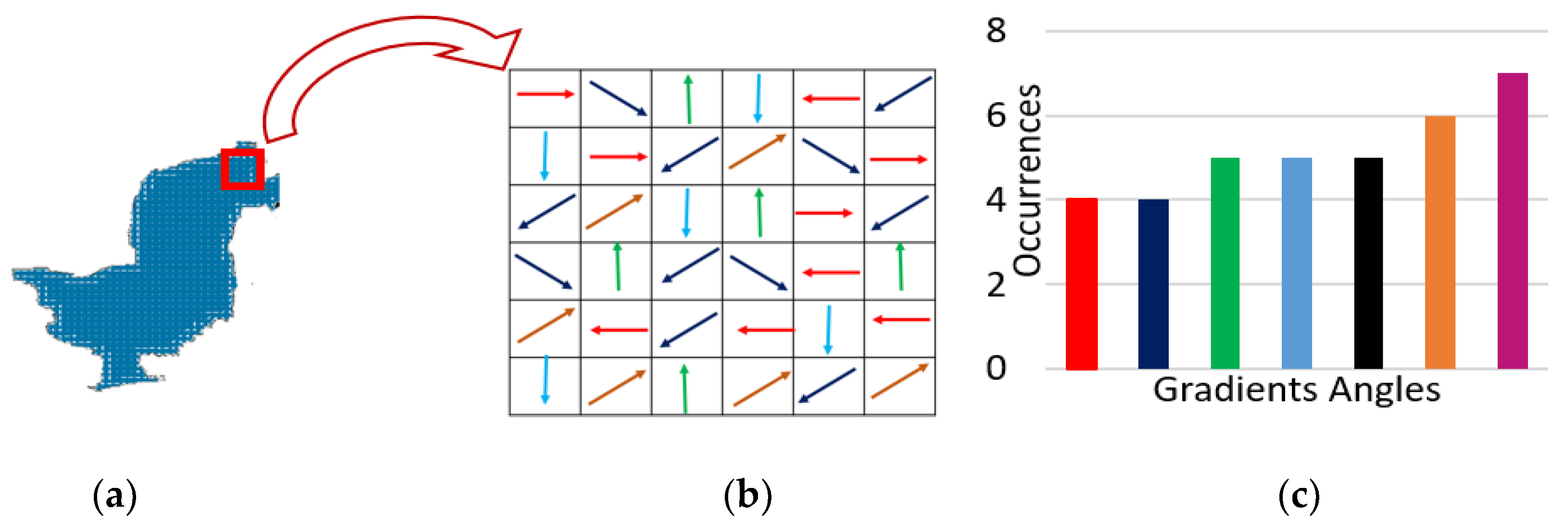
3.3.2. Gradient Kernel Descriptor over Segmented Objects

Changes in the direction of intensity or color in an image are termed the “gradient”. These gradients may be used to extract information from images. The following kernel of a gradient match $K_{\mathrm{gradient}}$ is implemented to capture image variations [13,54]:

$$K_{\mathrm{gradient}}\left(U,V\right)={\displaystyle \sum }_{\hslash \in U}{\displaystyle \sum }_{{\hslash }^{\prime }\in V}\overline{m}\left(ℌ\right)\overline{m}\left({ℌ}^{\prime }\right){\kappa }_o\left(\overline{\vartheta }\left(ℌ\right),\overline{\vartheta }\left({ℌ}^{\prime }\right)\right){\kappa }_s\left(ℌ,{ℌ}^{\prime }\right)$$

(13)

where the Gaussian position kernel is symbolized as ${\kappa }_s\left(ℌ,{ℌ}^{\prime }\right)=\exp \left(-{\gamma }_s{\Vert ℌ-{ℌ}^{\prime }\Vert }^2\right)$, with a pixel location of $ℌ$ in the two-dimensional image patch (standardized to [0,1]), and kernel with respect to orientation is represented as ${\kappa }_o$($\vartheta$ e($ℌ$), $\vartheta$ e($ℌ$)) = exp(−${\gamma }_o{\Vert \overline{\vartheta }\left(ℌ\right)-\overline{\vartheta }\left({ℌ}^{\prime }\right)\Vert }^2$). To measure the disparity between the viewpoints of pixels $ℌ$ and ${ℌ}^{\prime }$, the following standardized gradient vector is imbedded in the kernel function ${\kappa }_o$:

$$\overline{\vartheta }\left(ℌ\right)=\left[\sin \left(\vartheta \left(ℌ\right)\right)\cos \left(\vartheta \left(ℌ\right)\right)\right]$$

(14)

The L2 distance between these vectors estimates well enough the disparity in gradient viewpoints. In some situations, it would be inappropriate to measure an L2 distance at a raw angle $\vartheta$ instead of standardized gradient vectors $\vartheta e$. For instance, consider both 2π–0.01 and 0.01 angles of a very similar inclination but a larger L2 width.

To conclude, the gradient match kernel $K_{\mathrm{gradient}}$ comprises three kernels: standardized linear kernel and orientation histogram kernels are identical, where gradient magnitudes are responsible for the assessment of every pixel’s impact—to enumerate the viewpoints’ similarity i.e., similarity of gradient orientation, ${\kappa }_o$ is computed—whereas the intimacy of two pixels is evaluated by the position Gaussian kernel ${\kappa }_s$. Figure 5 shows gradient KDES results over some example images of the datasets under consideration.

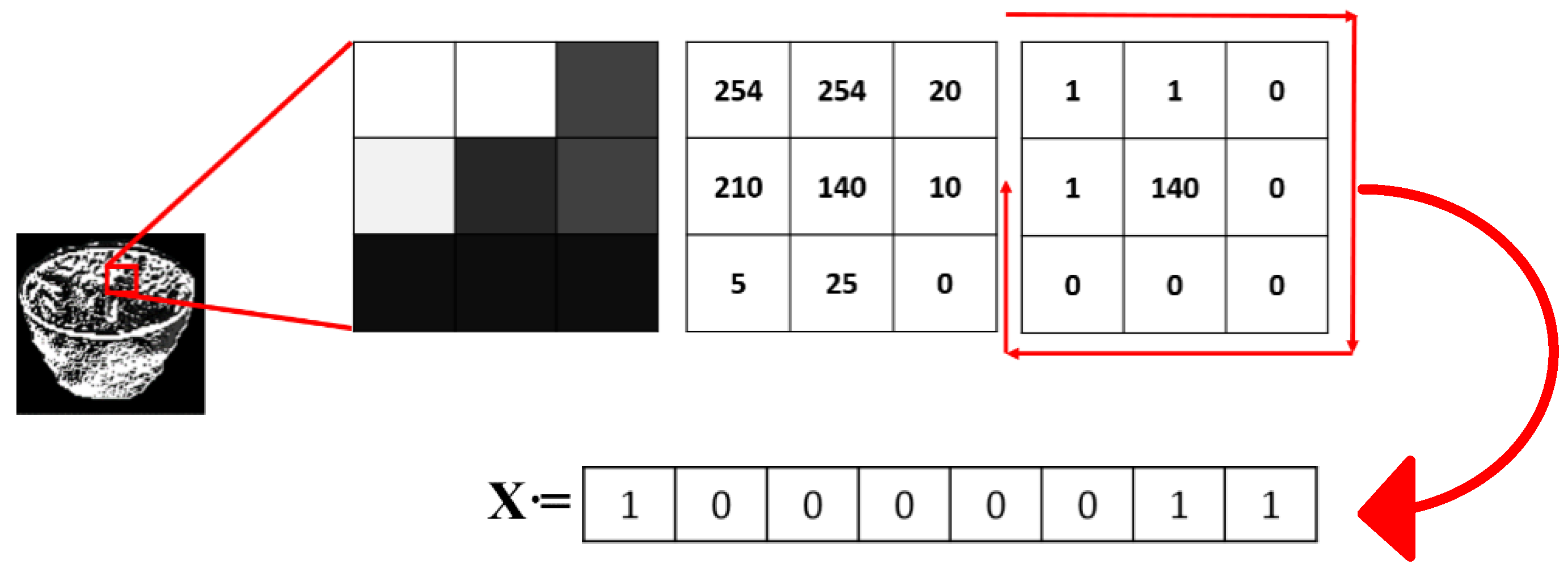
3.3.3. LBP Kernel Descriptor over Segmented Objects

Image variations are captured by the gradient match kernel, whereas it is observed that the local binary pattern (LBP) match kernel [45] is capable of capturing local structure.

$$K_{\mathrm{shape}}\left(A,B\right) = {\displaystyle \sum }_{Z\in A}{\displaystyle \sum }_{Z^{\prime }\in B}\tilde{s}\left(z\right)\tilde{s}\left(z^{\prime }\right)k_b\left(b\left(z\right),b\left(z^{\prime }\right)\right)k_p\left(z,z^{\prime }\right)$$

(15)

where the standard deviation is denoted as $\tilde{s}\left(z\right)=s\left(z\right)/\sqrt{{{\displaystyle \sum }}_{Z\in A}s{\left(z\right)}^2+{ϵ}_s}, s\left(z\right)$ nearby $z$, ${ϵ}_s$ in a window of 3 × 3, and b($z$) is called the binary column vector to binarize the pixel value dissimilarities around z. The significance of each LBP is measured by the standardized linear kernel $\tilde{s}\left(z\right)\tilde{s}\left(z^{\prime }\right)$, whereas the kernel $k_b\left(b\left(z\right),b\left(z^{\prime }\right)\right)=\exp \left(-{\gamma }_b{\Vert b\left(z\right)-b\left(z^{\prime }\right)\Vert }^2\right)$ is responsible for quantifying the likeness based on LBP. Figure 6 exhibits LBP KDES results in the form of histograms and Figure 7 explains the mathematical procedure of LBP.

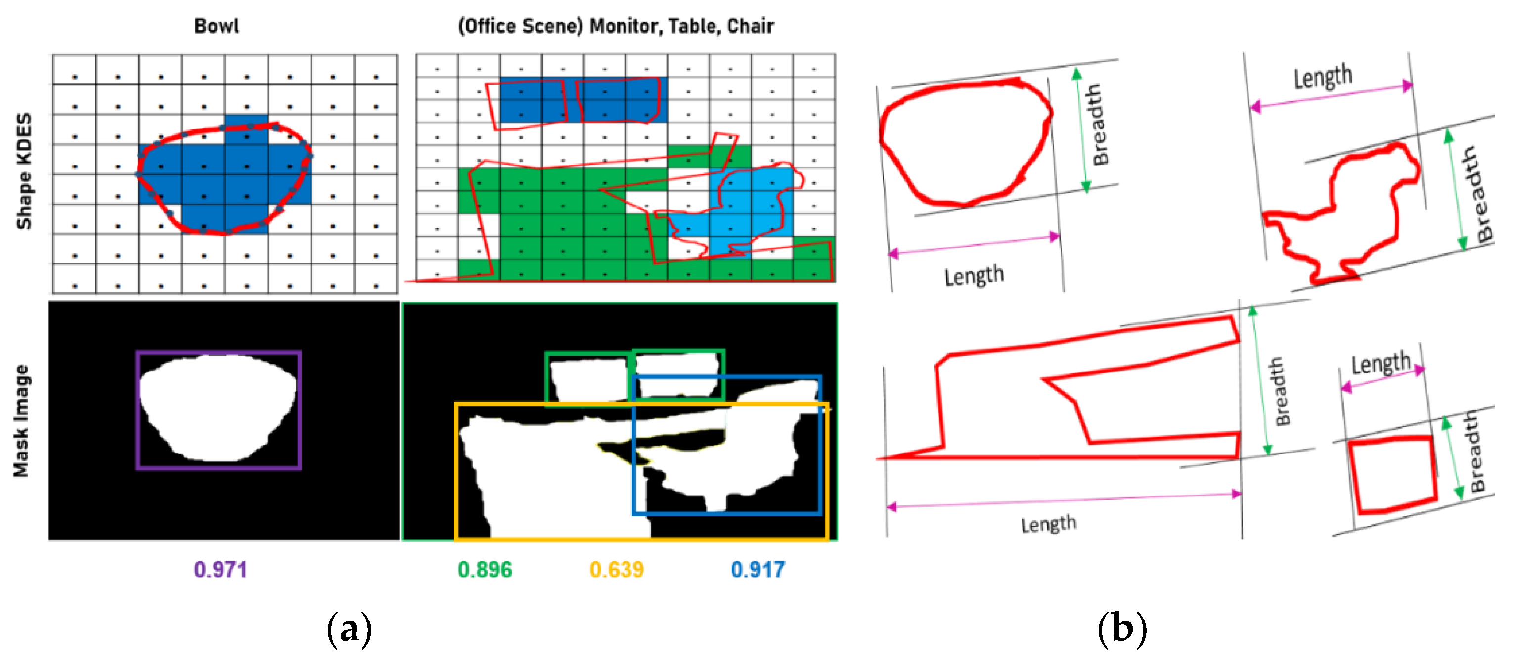
3.3.4. Kernel Principal Copponent Aanalysis (PCA) and Shape Kernel Descriptor over Segmented Objects

To capture objects, shape KDES is a strong descriptor for the recognition of instances and category recognition. We take two features into account as shape KDES, namely PCA KDES and spin features. Then, the kernel metrics of a bowl, chair, table, and monitor are examined. Later, the resultant matrix of computed eigenvalues are plotted against each object, as shown in Figure 8. The distribution of bowl, chair, table, and monitor values are presumed to be very different, implying that the particular values are likely to capture the 3D shape of objects. The kernel matrix $K_{pca}$ is evaluated over the point cloud $\wp$. We also computed the twenty-five highest eigenvalues $\mathcal{T}$, and attained $\left[{\mathsf{\Lambda }}_{\wp }^1,\dots ,{\mathsf{\Lambda }}_{\wp }^{𝓉},\dots ,{\mathsf{\Lambda }}_{\wp }^{\mathcal{T}}\right]$ as PCA KDES with:

$$K_{pca}{\mathrm{v}}^{𝓉}={\mathsf{\Lambda }}_{\wp }^{𝓉}{\mathrm{v}}^{𝓉}$$

(16)

where eigenvectors are represented by ${\mathrm{v}}^{𝓉}$, PCA KDES comprised $\mathcal{T}$ dimensions, and $K_{pca}\left[𝓍,𝓎\right]=\exp \left(-{\gamma }_k\parallel 𝓍-𝓎\right]{\parallel }^2)$ with ${\gamma }_k>0$ and $𝓍,𝓎\in \wp$.

To discriminate the shape of the object [67,68], the compactness of the object is estimated using Equation (17) and Equation (18):

$$C=\frac{\mathrm{A}\left(\mathrm{Obj}\right)}{\mathrm{A}\left(\mathrm{B}\_\mathrm{box}\right)}$$

(17)

$$\mathrm{A}\left(\mathrm{Obj}\right)=\frac{{{\displaystyle \sum }}_{i\in \mathit{Contour}}\left(x_i+x_{i-1}\right)\cdot \left(y_i-y_{i-1}\right)}{2}$$

(18)

where $C$ is compactness, $\mathrm{A}\left(\mathrm{Obj}\right)$ represents the area of the object, and $\mathrm{A}\left(\mathrm{B}\_\mathrm{box}\right)$ denotes the bounding box with the smallest area around the object. Considering (x,y) pixel locations in the image for a specific object, where $i\in \mathrm{Contour}$ of the object, $x_i$ represents any pixel at the x co-ordinate of the object residing on the contour and $x_{i-1}$ represents its previous pixel at the x coordinate. Similarly, $y_i$ and $y_{i-1}$ are the pixels at the y co-ordinate. Thus, Equation (18) determines the contour point around the segmented object. Figure 9 clarifies the computation of the compactness ratio.

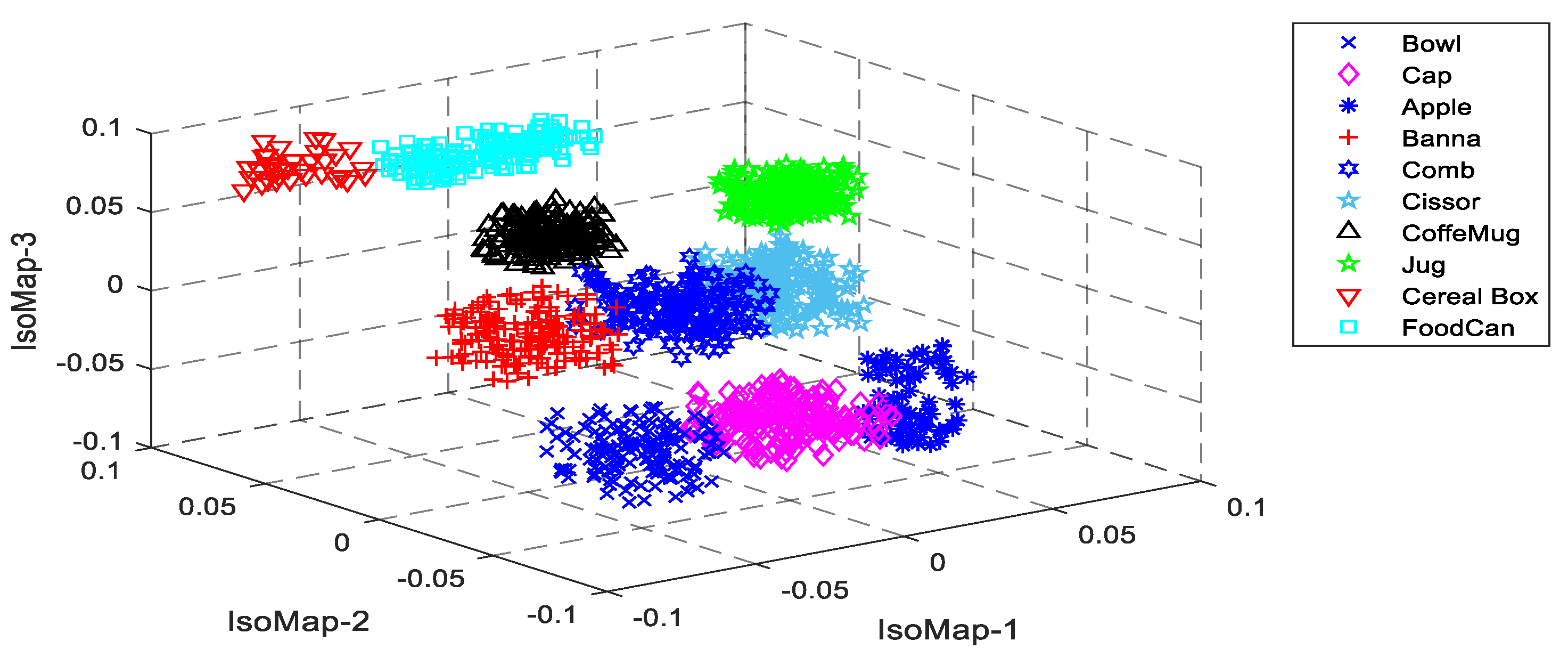
3.4. Feature Reduction using IsoMap

After feature extraction, to achieve maximum efficiency a feature reduction technique is applied. Feature reduction is vital for the recognition of objects. IsoMap [69,70] is an effective non-linear feature reduction technique that preserves the fundamental geometry of the data. The graph distance between the points is computed to measure the geodesic distances amongst the pixel pairs. IsoMap follows a similar idea to construct a matrix of similarity for a decomposition of eigenvalues. IsoMap constructs a similarity matrix based on local information contrary to other techniques, such as Locally-linear embedding (LLE) and log-likelihood probability (LLP). IsoMap estimates the geodesic distance by considering the shortest path between any two points that are taken from the neighborhood graph that is prepared using Euclidean distance. Consequently, the dimensions of the global and the local composition of the dataset are reduced (See Algorithm 2). Figure 10 illustrates the objects after feature reduction has been applied using IsoMap over the RGB-D object dataset.

Algorithm 2. Feature Extraction and Reduction.

3.5. Multi-Object Recognition

After feature extraction and reduction, the reduced feature space is then used to recognize the objects in the scene. The KSP, a unique classifier with a multi-layer perceptron, is applied for object recognition to enhance efficiency. After quantization, the feature vectors are passed to the KSP as inputs. The feature vectors are then transformed by the kernel into a transitional space based on computed feature pairs dot products as:

$$\mathrm{C}\left(z\right)={\arg }_i max\mathrm{sign}\left(\sum _{j=1}^M\beta k\left(z_j,z\right)\right)$$

(19)

where M represents training examples, $i$ is the object class in the image or scene, and each object has an assigned weight $\beta$ which is scalar. For training examples in which there is a chance of error, it will be non-zero.

The proposed architecture of the KSP as presented in Figure 11, which reveals that it contains input, output, and hidden layers with the perceptron. The input layer takes the feature vectors after reduction from the IsoMap, whereas the output layer contains multiple perceptrons depending on the number of object-classes in the training dataset. Algorithm 3 explains the process of KSP for multi-object recognition.

Algorithm 3. Multi-Object Recognition by Kernel Sliding Perceptron (KSP).

1:  Input: Reduced features set from RGB-D images 2:  Output: Yj Recognized Multi-object in a RGB-D image 3:  % set Max. # of repetitions% 4:  m = number of repetitions  $\beta =\beta 1,\dots ,\beta n$ 5:  Initialize $\beta j=0$ for every j 6:  WHILE ((t) and k <= n)       a.  t = 0;       b.  for (k = 1: m)             i.  if $y_j^{*}({\sum }_{i=1}^m {\alpha }_{l}k(z_j,z_l\left)\right) \le 0$             ii.  t = t + 1;             iii.  $\beta j=\beta j-1$+ $yjzj$             iv.  end       c.  end 7:  k = k + 1; 8:  end 9:  return Y

4. Experimental Setup and Results

Testing and validation of the proposed model were performed on three benchmark datasets: RGB-D objects, RGB-D scenes, NYU-Dv1 datasets. We executed four different sets of experiments for significant validation. For these experiments, the k-fold cross-validation method was employed, where k = 10. During this validation method, 9 of the 10 samples/images were used as training data and a single sample was taken for testing. The process was repeated 10 times. Datasets with more images were similarly distributed into subsets for the purpose of validation. Descriptions of the datasets used follow.

4.1. Datasets Descriptions

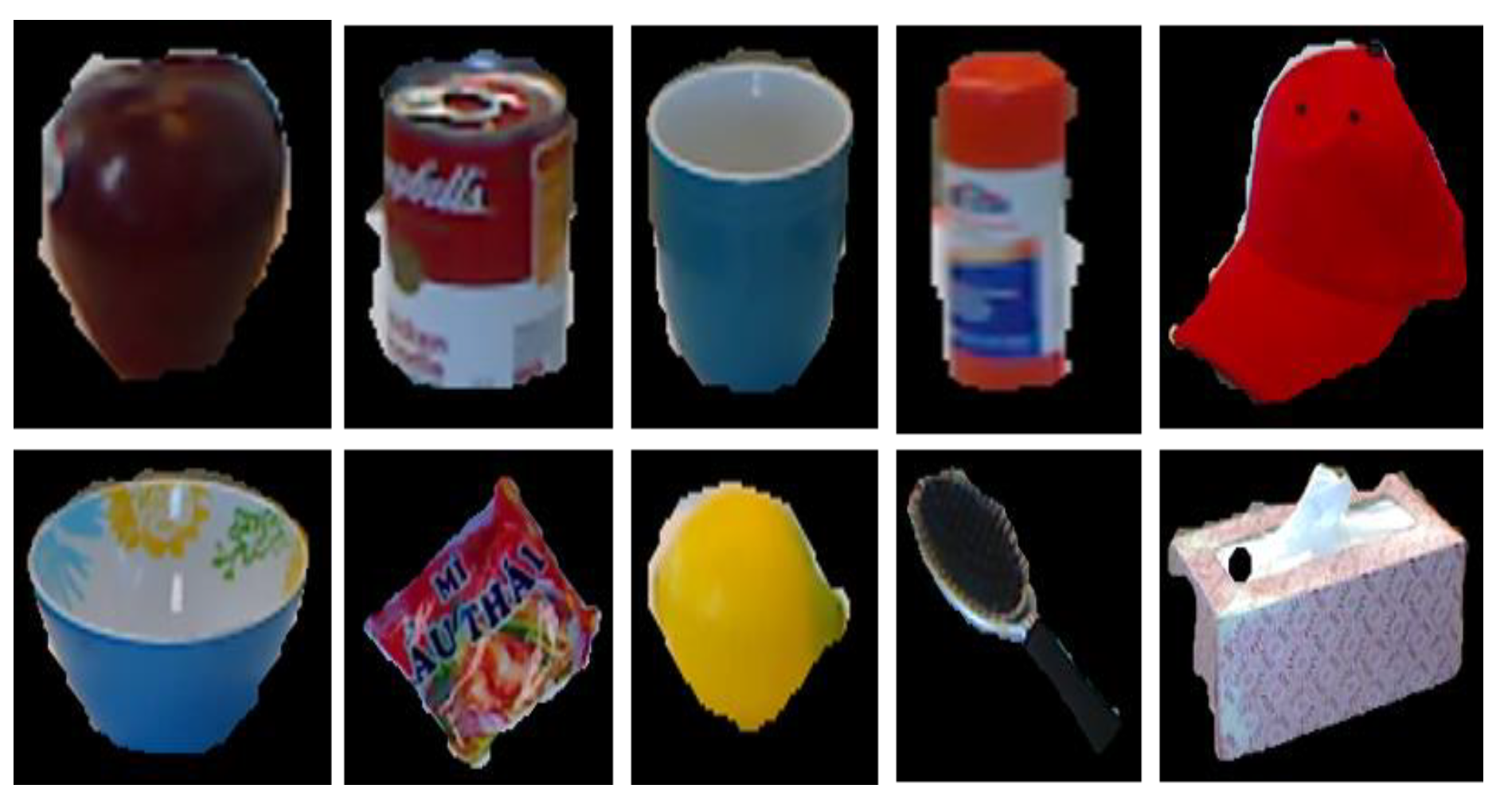
4.1.1. The RGB-D Object Dataset

The RGB-D object dataset [71] holds 300 collective household objects categorized into fifty-one unique types. These objects are organized into categories and instances. To record the dataset, a Kinect 3D camera was used to capture 640 × 480 RGB images, and depth images were recorded at 30 Hz. The objects were captured from different angles by rotating and changing the height of the camera. We considered 10 complex categories in the experimental evaluation: apple, bowl, banana, cap, comb, coffee mug, cereal box, food can, jug, and scissors. Figure 12 shows the example images form the RGB-D object dataset; these are complex images viewed from different angles from the horizon.

4.1.2. The RGB-D Scenes Dataset

The RGB-D scenes dataset [72] comprised fourteen scenes of furniture and other household objects. The RGB-D object dataset is also included as the subset of the RGB-D scenes dataset. The furniture scene is subdivided into chair, coffee table, sofa, and table, whereas the objects were bowl, cap, cereal box, coffee mug, and soda can. Figure 13 depicts a example images from the RGB-D scenes dataset.

4.1.3. The NYU-Dv1 Dataset

The NYUDv1 dataset [73] comprises 2347 labeled and 108,617 unique unlabeled frames of seven types with 64 different indoor scenes. These frames/scenes are grouped into the following seven classes: bathroom, bedroom, bookstore, café, kitchen, living room, and office. These classes consist of different objects, including bed, bookshelf, book, cabinet, ceiling, floor, picture, sofa, table, TV, wall, window, background, and unlabeled. Examples from the NYUDv1 dataset are presented in Figure 14.

4.2. First Experiment: Recognition Accuracy

The first experiment was performed on three publicly available datasets to determine the efficiency of the proposed model using a KSP.

4.2.1. Experimental Setup

In this experiment, the three DKDES, i.e., gradient KDES, PCA KDES, and size KDES, were applied for single object recognition, using the RGB-D object dataset, whereas five DKDES, i.e., gradient, kernel PCA, size, shape, and local binary pattern KDES were applied to a KSP for multiple object recognition using the RGB-D scenes and NYU-Dv1 datasets. To measure the performance of the proposed model over the three benchmark datasets, the experiment was repeated three times.

Table 1. Confusion matrix for recognition accuracy over the RGB-D object dataset.

Obj. Classes	bow	ban	app	cap	com	fcn	cmg	jug	cbx	scs
bow	0.97	0.00	0.00	0.00	0.00	0.00	0.03	0.00	0.00	0.00
ban	0.00	0.96	0.00	0.00	0.04	0.00	0.00	0.00	0.00	0.00
app	0.05	0.00	0.95	0.00	0.00	0.00	0.00	0.00	0.00	0.00
cap	0.03	0.00	0.00	0.93	0.00	0.04	0.00	0.00	0.00	0.00
com	0.00	0.08	0.00	0.00	0.90	0.00	0.00	0.00	0.00	0.02
ccn	0.00	0.00	0.00	0.00	0.00	0.87	0.00	0.00	0.13	0.00
cmg	0.03	0.00	0.00	0.00	0.00	0.00	0.83	0.14	0.00	0.00
jug	0.00	0.00	0.00	0.00	0.00	0.08	0.00	0.92	0.00	0.00
cbx	0.00	0.00	0.00	0.02	0.00	0.07	0.00	0.00	0.93	0.00
scs	0.00	0.05	0.00	0.00	0.00	0.00	0.00	0.00	0.00	0.95
Mean Accuracy = 92.16%

bow = bowl; ban = banana; app = apple; cap = cap; com = comb; fcn = food can; cmg = coffee mug; jug = jug; cbx = cereal box; scs = scissors.

demonstrates a confusion matrix over the RGB-D object dataset for single object recognition. An average recognition accuracy of 92.16% was reported over the RGB-D object dataset where we executed three kernels and 25 iterations for the experiment. Average recognition accuracies of 88.5% and 90.5% were achieved over the RGB-D scenes and the NYU-Dv1 datasets using three kernels and 25 iterations as depicted in

Table 2. Confusion matrix for recognition accuracy over the NYUDv1 dataset.

Obj. Classes	bed	bok	cab	cel	flr	sof	tab	tvn	wal	Win
bed	0.89	0.00	0.00	0.00	0.00	0.00	0.11	0.00	0.00	0.00
bok	0.00	0.86	0.00	0.00	0.00	0.00	0.00	0.14	0.00	0.00
cab	0.05	0.00	0.81	0.00	0.00	0.00	0.00	0.00	0.14	0.00
cel	0.00	0.00	0.00	0.85	0.00	0.00	0.00	0.00	0.15	0.00
flr	0.05	0.00	0.00	0.00	0.95	0.00	0.00	0.00	0.00	0.04
sof	0.00	0.00	0.00	0.00	0.00	0.81	0.12	0.00	0.07	0.00
tab	0.04	0.00	0.00	0.00	0.00	0.00	0.96	0.00	0.00	0.00
tvn	0.00	0.05	0.00	0.00	0.00	0.00	0.00	0.95	0.00	0.00
wal	0.00	0.00	0.00	0.07	0.00	0.00	0.00	0.00	0.87	0.06
win	0.00	0.00	0.00	0.00	0.00	0.00	0.00	0.00	0.10	0.90
Mean Accuracy = 88.5%

bed = bed; bok = book; cab = cabinet; cel = ceiling; flr = floor; sof = sofa; tab = table; tvn = television; wal = wall; win = window.

and

Table 3. Confusion matrix for recognition accuracy on multiple objects over the RGB-D scenes dataset.

Obj. Classes	chr	ctl	sof	tab	bow	cap	cbx	cmg	scn	wal	flr
chr	0.87	0.00	0.13	0.00	0.00	0.00	0.00	0.00	0.00	0.00	0.00
ctl	0.00	0.82	0.00	0.18	0.00	0.00	0.00	0.00	0.00	0.00	0.00
sof	0.17	0.00	0.83	0.00	0.00	0.00	0.00	0.00	0.00	0.00	0.00
tab	0.00	0.18	0.00	0.82	0.00	0.00	0.00	0.00	0.00	0.00	0.00
bow	0.00	0.00	0.00	0.04	0.96	0.00	0.00	0.00	0.00	0.00	0.00
cap	0.00	0.00	0.00	0.00	0.00	0.88	0.00	0.12	0.00	0.00	0.00
cbx	0.00	0.00	0.00	0.00	0.00	0.00	0.77	0.09	0.14	0.00	0.00
cmg	0.00	0.00	0.00	0.00	0.00	0.21	0.00	0.79	0.00	0.00	0.00
scn	0.00	0.00	0.00	0.00	0.00	0.00	0.09	0.26	0.65	0.00	0.00
wal	0.00	0.00	0.00	0.00	0.00	0.00	0.00	0.00	0.00	0.86	0.14
flr	0.00	0.00	0.00	0.00	0.00	0.00	0.00	0.00	0.00	0.20	0.80
Mean Accuracy = 90.5%

chr = chair; ctl = coffee table; sof = sofa; tab = table; bow = bowl; cap = cap; cbx = cereal box; cmg = coffee mug; scn = soda can; wal = wall; flr = floor.

, respectively.

We considered five kinds of depth KDES, namely, size KDES, shape KDES, gradient KDES, LBP KDES, and PCA KDES to recognize multiple objects from the three benchmark datasets out of which the RGB-D object was used to recognize a single object by applying three DKDES. Figure 15 demonstrates that accuracy increased with an increase in the number of kernels in both cases, for either single or multi-object recognition. For single object recognition, the order of the selected depth descriptors is shape KDES, PCA KDES, and LBP KDES, whereas for multi-object recognition, the order is size KDES, shape KDES, gradient KDES, LBP KDES, and PCA KDES. A combination of all five DKDES outperforms the accuracy rates of current state-of-the-art methods.

4.2.2. Observations

Experimental results reveal that the commended KDES can recognize objects using a KSP. For single object recognition, the highest accuracy was obtained over the RGB-D object dataset. Due to the increased number of DKDES, average recognition accuracy for multi-object recognition is nearly equal to single object recognition. A similar trend is observed in the performance analysis of all of the datasets under consideration. Although some misperception occurred for similar objects, such as the coffee mug, soda can, sofa and chair, most of the results are significant. It can also be observed that the experimental findings change as the number of kernels and repetitions of the classifier vary. Hence, computational time with variants of kernel and repetitions is assessed in the second experiment to evaluate the effect of specific kernels and iterations on recognition results.

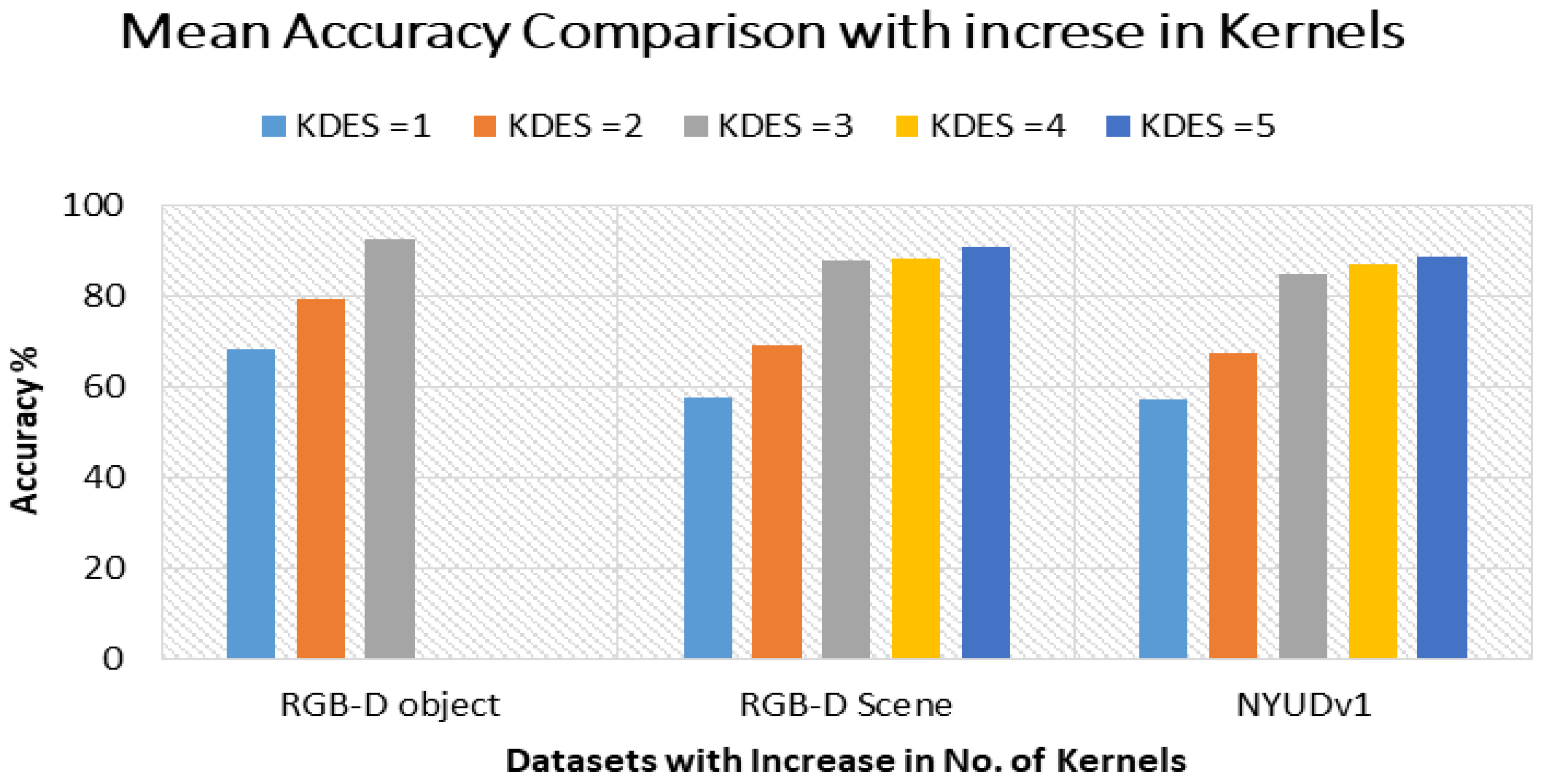
4.3. Second Experiment: Level of Kernels

The second experiment was conducted to validate variations in the kernels and iterations for the three standard and publicly available datasets, using the KSP.

Experimental Setup

To validate our statement that increases in the number of kernels may increase recognition efficiency, several experiments were completed. These experiments compared the performance in terms of accuracy and computational time. Firstly, to evaluate recognition accuracy and computational time, the experiment was conducted by considering only one kernel, and keeping iterations from 10 to 25. The above experiments were repeated for two and three kernels, respectively.

Table 4. Computational time of the proposed system using K = 1, 2, and 3 for recognition over the RGB-D object dataset.

Parameters	Performance
Kernels	Iterations	Accuracy (%)	Comp. Time (s)
k = 1	i = 10	85.76	1.93
	i = 15	85.94	2.17
	i = 20	86.47	2.82
	i = 25	86.89	3.21
k = 2	i = 10	87.21	3.97
	i = 15	87.96	4.56
	i = 20	88.32	4.89
	i = 25	89.03	5.14
k = 3	i = 10	90.55	5.78
	i = 15	91.14	6.49
	i = 20	91.95	6.86
	i = 25	92.20	7.65

,

Table 5. Computational time of proposed system by using K = 1, 2, and 3 for recognition over RGB-D Scenes dataset.

Parameters	Performance
Kernels	Iterations	Accuracy (%)	Comp. Time (s)
k = 1	i = 10	82.16	1.63
	i = 15	82.94	1.97
	i = 20	83.47	2.52
	i = 25	84.62	2.89
k = 2	i = 10	85.51	3.17
	i = 15	86.36	3.68
	i = 20	86.91	4.01
	i = 25	87.65	4.59
k = 3	i = 10	88.58	4.95
	i = 15	89.97	5.31
	i = 20	90.50	5.81
	i = 25	90.05	6.11

and

Table 6. Computational time of proposed system by using Kernel = 1, 2, and 3 for object recognition over NYUDv1 dataset.

Parameters	Performance
Kernels	Iterations	Accuracy (%)	Comp. Time (s)
k = 1	i = 10	81.95	1.35
	i = 15	82.74	1.99
	i = 20	83.31	2.41
	i = 25	83.89	2.87
k = 2	i = 10	84.82	3.13
	i = 15	85.19	3.56
	i = 20	85.91	4.03
	i = 25	86.77	4.75
k = 3	i = 10	87.29	5.16
	i = 15	87.98	5.95
	i = 20	88.50	6.12
	i = 25	88.12	6.84

demonstrate the experimental analyses of the results on RGB-D objects, RGB-D scenes, and NYUDv1 datasets, respectively.

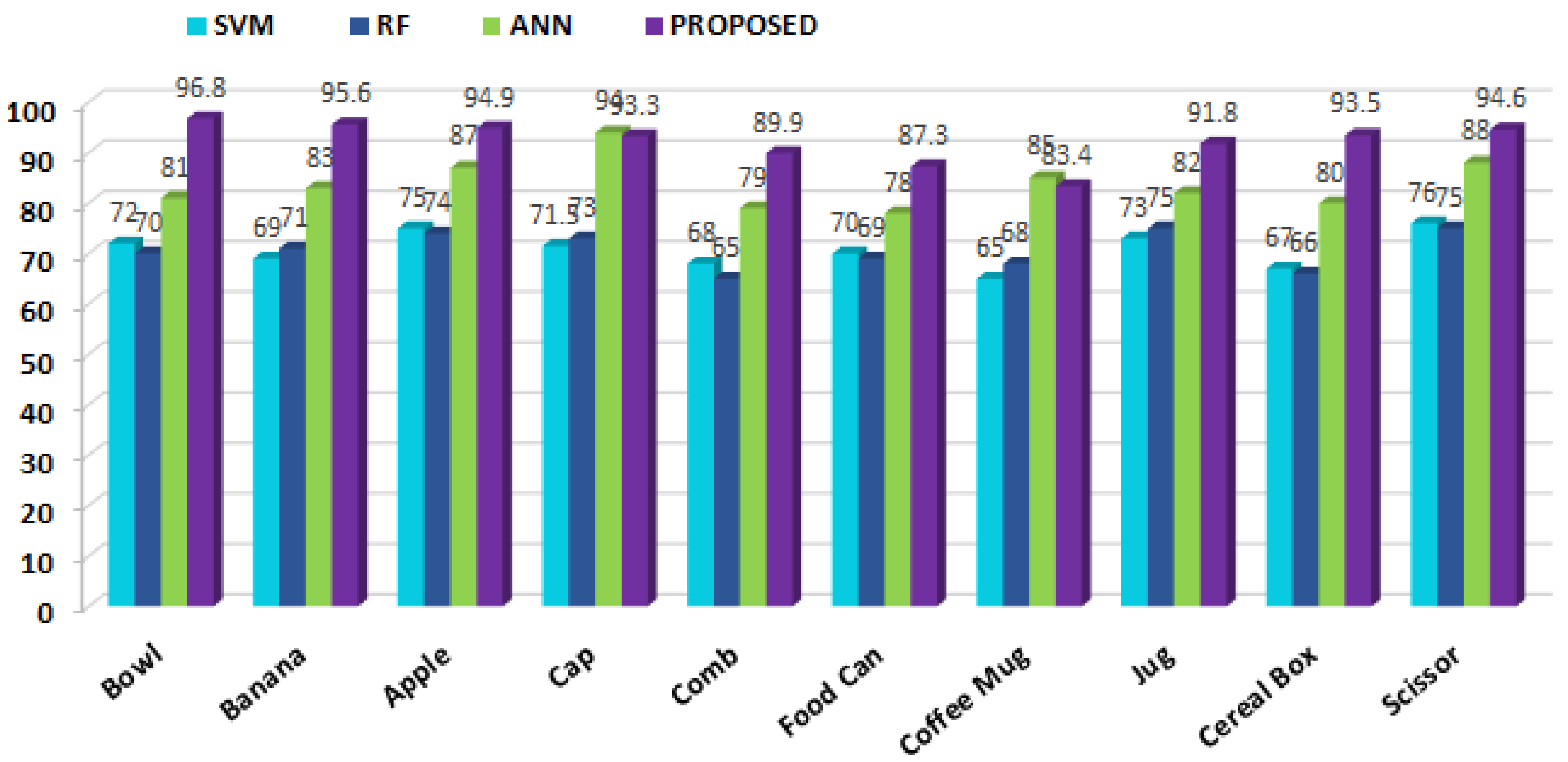
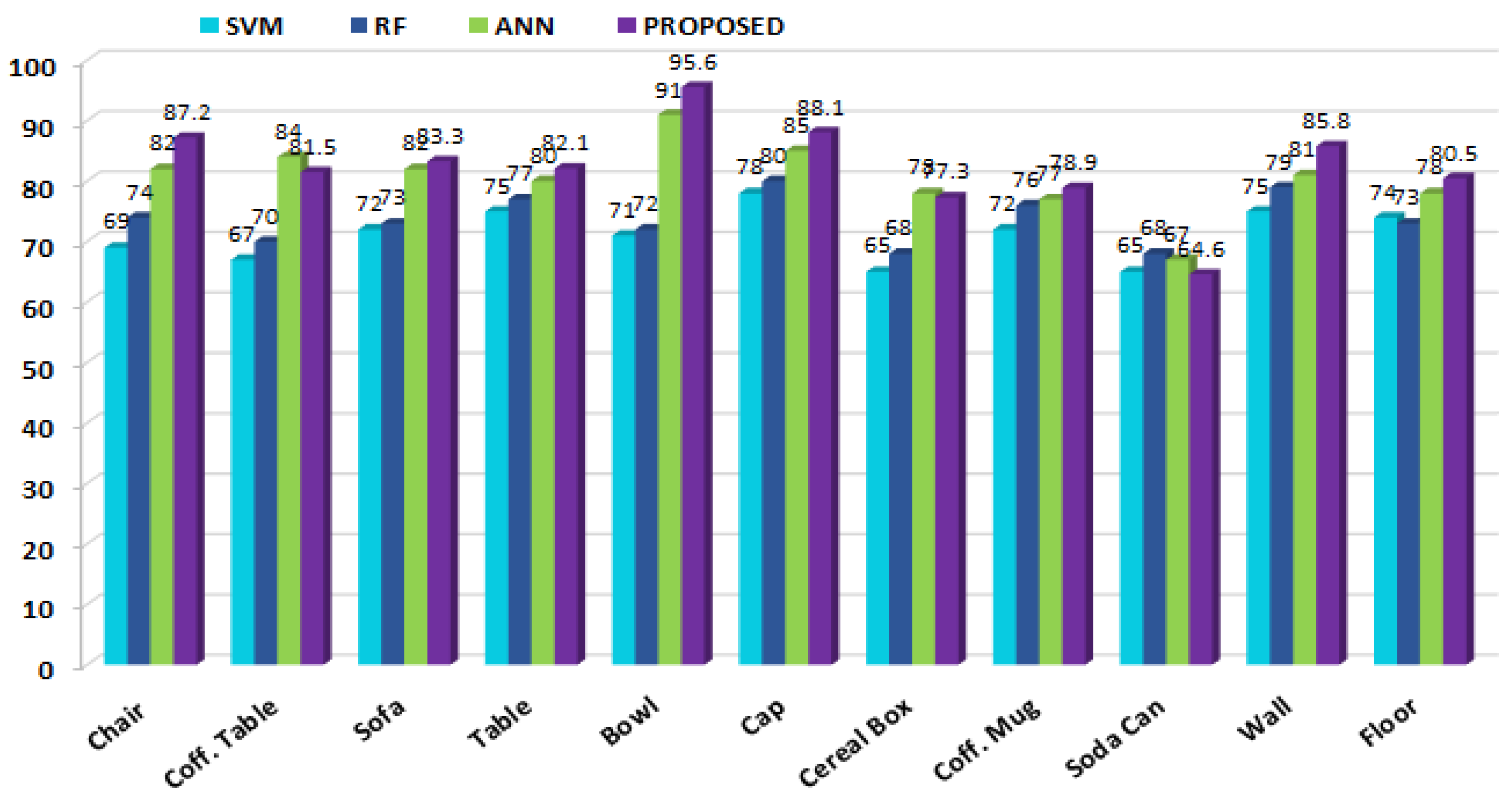
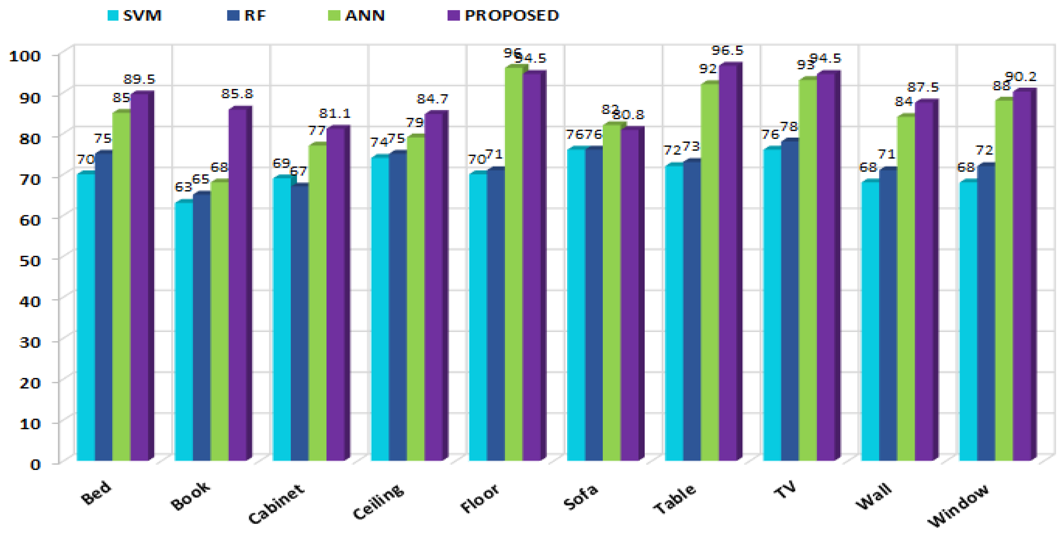
4.4. The Third Experiment: Conventional Methods vs. the Proposed Method

In the third experiment, depth kernel descriptors (depth KDES) were extended to all three benchmark datasets employing conventional approaches, namely, SVM, random forest (RF), and artificial neural network (ANN).

4.4.1. Experimental Setup

Three sub-experiments were carried out under this experiment on each of the benchmark datasets. Initially, a set of depth KDES were provided to the support vector machine (SVM) to recognize the objects. These depth KDES were then given to a random forest (RF) and artificial neural network (ANN) to obtain the object recognition results. Finally, the conventional approaches were compared to the proposed model using a KSP. Figure 16, Figure 17 and Figure 18 represent the comparison results over the RGB-D object, RGB-D scenes, and NYU-Dv1 datasets, respectively.

4.4.2. Observations

SVM, RF, and ANN achieved overall recognition accuracy rates of 70.7%, 70.6%, and 83.7%, respectively, for the RGB-D object dataset, whereas the proposed model with KSP achieved an accuracy rate of 92.2% for the same dataset. It is evident from Figure 16 that the proposed model using the multi-layer KSP obtained optimum output for the bowl and the banana, however, for the cap and the coffee mug, ANN performed better than the proposed model. This indicates that ANN is more suitable in certain situations; nevertheless, the overall recognition rate of KSP is superior to that of the ANN.

Similarly, using the SVM, RF, ANN, and KSP, an improvement in recognition accuracies is observed over the RGB-D scenes dataset with increases in the number of depth KDES of 78.3%, 81.0%, 88.5%, and 90.4%, respectively. It is evident from Figure 17 that the proposed model performed well on all of the objects, with the exception of the coffee table and cereal box, for which the ANN performed slightly better. The RF performed better on the soda can compared to both ANN and the proposed model. Nevertheless, the proposed model performed better on all of the other objects, i.e., the proposed model performed significantly better overall.

4.5. Fourth Experiment: Comparison with the Latest Techniques

The fourth experiment performed comparisons of our method with state-of-the-art methods for object recognition in depth images.

Table 7. Comparison of object recognition accuracy over RGB-D object dataset (by applying three DKDES), RGB-D scenes, and NYUDv1 datasets (by applying five DKDES).

Method	Accuracy on Single Object %	Accuracy on Multi-Object (%)
	RGB-D Object	RGB-D Scenes	NYUDv1
Saliency map [19]	86.9	-	-
AlexNet-RNN [72]	90.9	-	-
3DEF-FFSM [73]	-	-	52.6
Fus-CNN(jet) [70]	91.3	-	-
MM-ELM-LRF [71]	89.3	-	-
CRF [69]	-	-	56.6
STEM-CaRFs [18]	92.2	81.7	-
Deep CNN [12]	91.8	-	-
Full 2D Segmentation [71]	-	-	59.5
HMP3D [68]	-	82.1	-
Proposed	92.2	90.5	88.5

presents the comparison results over RGB-D object, RGB-D scenes, and NYUDv1 datasets.

A. Ahmed et al. [19] proposed a saliency map fused with centered darker channel-based RGB-D object segmentation to recognize the objects in indoor scenarios. They extracted histogram of oriented gradients (HOG) features after the point cloud conversion of segmented images. Finally, they used Hough voting for the recognition of the object. H. Liu et al. [21] presented a multi-modal architecture named MM-ELM-LRF. They extracted features for both of the modalities (RGB and depth) by applying ELM-LRF. Then, by fusing features from these modalities, supervised feature classification was applied on the RGB-D object dataset for decision making. K. Lai et al. [67] presented a new approach to the labelling of 3D scenes by employing Hierarchical matching pursuit for 3D (HMP3D) to extract and learn the features from point clouds. Their model integrates the features from RGB-D images and point clouds, and assigns a label to each 3D point in the scene. They validated their model on the RGB-D scenes dataset and recommended their system for both small indoor objects and furniture recognition. N. Silberman et al. [69] discovered that the Microsoft Kinect depth sensor can support indoor scene segmentation. They also introduced a new challenging dataset comprised of indoor scenes. The dataset also covers depth maps and dense labels. Additionally, to determine various representations of depth data, they used a Conditional Random Field (CRF) based model. They evaluated their model on the newly proposed RGB-D scenes dataset. A. Eital et al. [70] proposed a robust method for RGB-D object detection using a convolutional neural network (CNN). They combined two different processing streams via a fusion network. They also incorporated a multi-stage training mechanism with effective encoding and data augmentation for robust learning. They achieved 91.3% recognition accuracy over the RGB-D object dataset.A. Hermans et al. [71] suggested a 2D–3D label transfer based on Bayesian updates and 3D conditional random fields. They also proposed a 2D semantic segmentation approach based on randomized decision forests. A. Caglayan et al. [72] presented a two-stage framework that used multi-model RGB-D images to extract discriminative feature representations for object and scene recognition. M. Antonello et al. [73] contributed a multi-view frame fusion method and batch system to enhance the semantic labels. This fusion method uses an incremental mode to generate single view results. It performs semantic segmentation of single frames and semantic map reconstruction.

5. Conclusions

In this paper, we introduced a novel sustainable framework to recognize objects in complex depth environments. Key achievements, such as the sustainable segmentation of indoor scene depth objects, and a combination of robust extraction of DKDES and KSP for distinguishing each object, were attained in this study. The impact and significance of the proposed model compared to previous techniques is highlighted, with recognition accuracies of 92.2%, 88.5%, and 90.5% over RGB-D object samples, RGB-D scenes, and NYUDv1 datasets, respectively. Moreover, results suggest that our proposed technique is ideal for object recognition despite any change in the environment, evidenced by consistent results. It can be adopted in numerous applications, such as medical diagnostics, video surveillance, robotic navigation, and understanding of indoor scenes.

In the future, we plan to improve our model by considering contextual and semantic segmentation using deep learning techniques. Similarly, dynamic scenarios will be considered with the use of a combined classifiers technique for efficient application.

References

1. Ly, H.-B.; Le, T.-T.; Vu, H.-L.T.; Tran, V.Q.; Le, L.M.; Pham, B.T. Computational Hybrid Machine Learning Based Prediction of Shear Capacity for Steel Fiber Reinforced Concrete Beams. Sustainability 2020, 12, 2709. [Google Scholar] [CrossRef] [Green Version]
2. Cioffi, R.; Travaglioni, M.; Piscitelli, G.; Petrillo, A.; De Felice, F. Artificial Intelligence and Machine Learning Applications in Smart Production: Progress, Trends, and Directions. Sustainability 2020, 12, 492. [Google Scholar] [CrossRef] [Green Version]
3. Buenestado, P.; Acho, L. Image Segmentation Based on Statistical Confidence Intervals. Entropy 2018, 20, 46. [Google Scholar] [CrossRef] [Green Version]
4. Khan, M.W. A Survey: Image Segmentation Techniques. Int. J. Futur. Comput. Commun. 2014, 3, 89. [Google Scholar] [CrossRef] [Green Version]
5. Dhanachandra, N.; Chanu, Y.J. A Survey on Image Segmentation Methods using Clustering Techniques. Eur. J. Eng. Res. Sci. 2017, 2, 15–20. [Google Scholar] [CrossRef] [Green Version]
6. Alata, O.; Quintard, L. Is there a best color space for color image characterization or representation based on Multivariate Gaussian Mixture Model? Comput. Vis. Image Underst. 2009, 113, 867–877. [Google Scholar] [CrossRef]
7. Pagola, M.; Ortiz, R.; Irigoyen, I.; Bustince, H.; Barrenechea, E.; Aparicio-Tejo, P.; Lamsfus, C.; Lasa, B. New method to assess barley nitrogen nutrition status based on image colour analysis. Comput. Electron. Agric. 2009, 65, 213–218. [Google Scholar] [CrossRef]
8. Jurio, A.; Pagola, M.; Galar, M.; Lopez-Molina, C.; Paternain, D. A comparison study of different color spaces in clustering based image segmentation. In International Conference on Information Processing and Management of Uncertainty in Knowledge-Based Systems; Springer: Berlin/Heidelberg, Germany, 2010; pp. 532–541. [Google Scholar]
9. Sinop, A.K.; Grady, L. A seeded image segmentation framework unifying graph cuts and random walker which yields a new algorithm. In Proceedings of the 2007 IEEE 11th International Conference on Computer Vision, Rio de Janeiro, Brazil, 14–21 October 2007; pp. 1–8. [Google Scholar]
10. Rashid, M.; Khan, M.A.; Alhaisoni, M.; Wang, S.-H.; Naqvi, S.R.; Rehman, A.; Saba, T. A Sustainable Deep Learning Framework for Object Recognition Using Multi-Layers Deep Features Fusion and Selection. Sustainability 2020, 12, 5037. [Google Scholar] [CrossRef]
11. Ahmed, A.; Jalal, A.; Rafique, A.A. Salient Segmentation based Object Detection and Recognition using Hybrid Genetic Transform. In Proceedings of the 2019 International Conference on Applied and Engineering Mathematics (ICAEM), Taxila, Pakistan, 27–29 August 2019; pp. 203–208. [Google Scholar]
12. Zia, S.; Yüksel, B.; Yuret, D.; Yemez, Y. RGB-D object recognition using deep convolutional neural networks. In Proceedings of the 2017 IEEE International Conference on Computer Vision Workshops, Venice, Italy, 22–29 October 2017. [Google Scholar]
13. Ahmed, A.; Jalal, A.; Kim, K. A Novel Statistical Method for Scene Classification Based on Multi-Object Categorization and Logistic Regression. Sensors 2020, 20, 3871. [Google Scholar] [CrossRef]
14. Bo, L.; Ren, X.; Fox, D. Kernel descriptors for visual recognition. In Proceedings of the Advances in Neural Information Processing Systems 23: 24th Annual Conference on Neural Information Processing Systems 2010, Vancouver, BC, Canada, 6–9 December 2010; pp. 244–252. Available online: https://papers.nips.cc/paper/2010/hash/4558dbb6f6f8bb2e16d03b85bde76e2c-Abstract.html (accessed on 25 June 2020).
15. Venkatrayappa, D.; Montesinos, P.; Diep, D.; Magnier, B. A novel image descriptor based on anisotropic filtering. In International Conference on Computer Analysis of Images and Patterns; Springer: Cham, Switzerland, 2015; pp. 161–173. [Google Scholar]
16. Song, S.; Xiao, J. Sliding shapes for 3d object detection in depth images. In European Conference on Computer Vision; Springer: Cham, Switzerland, 2014; pp. 634–651. [Google Scholar]
17. Shi, W.; Zhu, D.; Zhang, G.; Chen, L.; Wang, L.; Li, J.; Zhang, X. Multilevel Cross-Aware RGBD Semantic Segmentation of Indoor Environments. In Proceedings of the 2019 IEEE International Conference on Cyborg and Bionic Systems (CBS), Munich, Germany, 18–20 September 2019; pp. 346–351. [Google Scholar]
18. Asif, U.; Bennamoun, M.; Sohel, F.A. RGB-D object recognition and grasp detection using hierarchical cascaded forests. IEEE Trans. Robot. 2017, 33, 547–564. [Google Scholar] [CrossRef] [Green Version]
19. Ahmed, A.; Jalal, A.; Kim, K. RGB-D images for object segmentation, localization and recognition in indoor scenes using feature descriptor and Hough voting. In Proceedings of the 2020 17th International Bhurban Conference on Applied Sciences and Technology (IBCAST), Islamabad, Pakistan, 14–18 January 2020; pp. 290–295. [Google Scholar]
20. Tang, L.; Yang, Z.-X.; Jia, K. Canonical Correlation Analysis Regularization: An Effective Deep Multiview Learning Baseline for RGB-D Object Recognition. IEEE Trans. Cogn. Dev. Syst. 2019, 11, 107–118. [Google Scholar] [CrossRef]
21. Liu, H.; Li, F.; Xu, X.; Sun, F. Multi-modal local receptive field extreme learning machine for object recognition. Neurocomputing 2018, 277, 4–11. [Google Scholar] [CrossRef]
22. Hasan, M.M.; Mishra, P.K. Improving morphology operation for 2D hole filling algorithm. Int. J. Image Process. (IJIP) 2012, 6, 635–646. [Google Scholar]
23. Cho, J.-H.; Song, W.; Choi, H.; Kim, T.; Kim, T. Hole filling method for depth image based rendering based on boundary decision. IEEE Signal Process. Lett. 2017, 24, 329–333. [Google Scholar] [CrossRef]
24. Tingting, Y.; Junqian, W.; Lintai, W.; Yong, X. Three-stage network for age estimation. CAAI Trans. Intell. Technol. 2019, 4, 122–126. [Google Scholar] [CrossRef]
25. Zhu, C.; Miao, D. Influence of kernel clustering on an RBFN. CAAI Trans. Intell. Technol. 2019, 4, 255–260. [Google Scholar] [CrossRef]
26. Guo, X.; Xiao, J.; Wang, Y. A survey on algorithms of hole filling in 3D surface reconstruction. Vis. Comput. 2018, 34, 93–103. [Google Scholar] [CrossRef]
27. Jin, Z.; Tillo, T.; Zou, W.; Li, X.; Lim, E.G. Depth image-based plane detection. Big Data Anal. 2018, 3, 10. [Google Scholar] [CrossRef]
28. Li, L.; Sung, M.; Dubrovina, A.; Yi, L.; Guibas, L.J. Supervised fitting of geometric primitives to 3d point clouds. In Proceedings of the 2019 IEEE/CVF Conference on Computer Vision and Pattern Recognition (CVPR), Long Beach, CA, USA, 16–20 June 2019; pp. 2647–2655. [Google Scholar]
29. Anh-Vu, V.; Truong-Hong, L.; Debra; Laefer, F.; Bertolotto, M. Octree-based region growing for point cloud segmentation. ISPRS J. Photogramm. Remote Sens. 2015, 104, 88–100. [Google Scholar]
30. Dantanarayana, H.G.; Huntley, J.M. Object recognition in 3D point clouds with maximum likelihood estimation. In Automated Visual Inspection and Machine Vision; Nternational Society for Optics and Photonics: Munich, Germany, 2015; Volume 9530, p. 95300F. [Google Scholar]
31. Zhang, L.; Rastgar, H.; Wang, D.; Vincent, A. Maximum Likelihood Estimation sample consensus with validation of individual correspondences. In International Symposium on Visual Computing; Springer: Berlin/Heidelberg, Germany, 2009; pp. 447–456. [Google Scholar]
32. Zhao, B.; Hua, X.; Yu, K.; Xuan, W.; Chen, X.; Tao, W. Indoor Point Cloud Segmentation Using Iterative Gaussian Mapping and Improved Model Fitting. IEEE Trans. Geosci. Remote. Sens. 2020, 58, 7890–7907. [Google Scholar] [CrossRef]
33. Wiens, T. Engine speed reduction for hydraulic machinery using predictive algorithms. Int. J. Hydromechatronics 2019, 2, 16–31. [Google Scholar] [CrossRef]
34. Ádám, Á.; Chatzilari, E.; Nikolopoulos, S.; Kompatsiaris, I. H-RANSAC: A hybrid point cloud segmentation combining 2D and 3D data. ISPRS Ann. Photogramm. Remote. Sens. Spat. Inf. Sci. 2018, 4, 1–8. [Google Scholar] [CrossRef] [Green Version]
35. Barath, D.; Matas, J. Graph-Cut RANSAC. In Proceedings of the 2018 IEEE/CVF Conference on Computer Vision and Pattern Recognition, Salt Lake City, UT, USA, 18–23 June 2018; pp. 6733–6741. [Google Scholar] [CrossRef]
36. Kulkarni, S.M.; Bormane, D.S.; Nalbalwar, S.L. RANSAC algorithm for matching inlier correspondences in video stabilisation. Int. J. Signal Imaging Syst. Eng. 2017, 10, 178–184. [Google Scholar] [CrossRef]
37. Shokri, M.; Tavakoli, K. A review on the artificial neural network approach to analysis and prediction of seismic damage in infrastructure. Int. J. Hydromechatronics 2019, 2, 178–196. [Google Scholar] [CrossRef]
38. Gao, G.-Q.; Zhang, Q.; Zhang, S. Pose detection of parallel robot based on improved RANSAC algorithm. Meas. Control. 2019, 52, 855–868. [Google Scholar] [CrossRef] [Green Version]
39. Tran, N.-T.; Le Tan, F.-T.; Doan, A.-D.; Do, T.-T.; Bui, T.-A.; Tan, M.; Cheung, N.-M. On-device scalable image-based localization via prioritized cascade search and fast one-many ransac. IEEE Trans. Image Process 2018, 28, 1675–1690. [Google Scholar] [CrossRef]
40. Tahir, S.B.U.D.; Jalal, A.; Kim, K. Wearable Inertial Sensors for Daily Activity Analysis Based on Adam Optimization and the Maximum Entropy Markov Model. Entropy 2020, 22, 579. [Google Scholar] [CrossRef]
41. Shojaedini, E.; Majd, M.; Safabakhsh, R. Novel adaptive genetic algorithm sample consensus. Appl. Soft Comput. 2019, 77, 635–642. [Google Scholar] [CrossRef] [Green Version]
42. Carlos, G.; Martín, D.; Armingol, J.M. Joint object detection and viewpoint estimation using CNN features. In Proceedings of the 2017 IEEE International Conference on Vehicular Electronics and Safety (ICVES), Vienna, Austria, 27–28 June 2017; pp. 145–150. [Google Scholar]
43. Alqaisi, A.; Altarawneh, M.; Al, J.; Sharadqah, A.A. Analysis of color image features extraction using texture methods. TELKOMNIKA Telecommun. Comput. Electron. Control. 2019, 17, 1220–1225. [Google Scholar] [CrossRef] [Green Version]
44. Jalal, A.; Khalid, N.; Kim, K. Automatic Recognition of Human Interaction via Hybrid Descriptors and Maximum Entropy Markov Model Using Depth Sensors. Entropy 2020, 22, 817. [Google Scholar] [CrossRef]
45. Dadi, H.S.; Pillutla, G.K.M. Improved Face Recognition Rate Using HOG Features and SVM Classifier. IOSR J. Electron. Commun. Eng. 2016, 11, 34–44. [Google Scholar] [CrossRef]
46. Korkmaz, S.A.; Akcicek, A.; Binol, H.; Korkmaz, M.F. Recognition of the stomach cancer images with probabilistic HOG feature vector histograms by using HOG features. In Proceedings of the 2017 IEEE 15th International Symposium on Intelligent Systems and Informatics (SISY), Subotica, Serbia, 14–16 September 2017; pp. 000339–000342. [Google Scholar] [CrossRef]
47. Bheda, D.; Joshi, M.; Agrawal, V. A study on features extraction techniques for image mosaicing. Int. J. Innov. Res. Comput. Commun. Eng. 2014, 2, 3432–3437. [Google Scholar]
48. Jalal, A.; Kim, Y.-H.; Kim, Y.-J.; Kamal, S.; Kim, D. Robust human activity recognition from depth video using spatiotemporal multi-fused features. Pattern Recognit. 2017, 61, 295–308. [Google Scholar] [CrossRef]
49. Salahat, E.; Qasaimeh, M. Recent advances in features extraction and description algorithms: A comprehensive survey. In Proceedings of the 2017 IEEE International Conference on Industrial Technology (ICIT), Toronto, ON, Canada, 22–25 March 2017; pp. 1059–1063. [Google Scholar]
50. Bo, L.; Lai, K.; Ren, X.; Fox, D. Object recognition with hierarchical kernel descriptors. In Proceedings of the CVPR 2011, Providence, RI, USA, 20–25 June 2011; pp. 1729–1736. [Google Scholar]
51. Wang, P.; Wang, J.; Zeng, G.; Xu, W.; Zha, H.; Li, S. Supervised kernel descriptors for visual recognition. In Proceedings of the IEEE Conference on Computer Vision and Pattern Recognition, Portland, OR, USA, 23–28 June 2013; pp. 2858–2865. [Google Scholar]
52. Jalal, A.; Batool, M.; Kim, K. Stochastic Recognition of Physical Activity and Healthcare Using Tri-Axial Inertial Wearable Sensors. Appl. Sci. 2020, 10, 7122. [Google Scholar] [CrossRef]
53. Rafique, A.A.; Jalal, A.; Ahmed, A. Scene Understanding and Recognition: Statistical Segmented Model using Geometrical Features and Gaussian Naïve Bayes. In Proceedings of the IEEE Conference on International Conference on Applied and Engineering Mathematics, Taxila, Pakistan, 27–29 August 2019; Volume 57, pp. 225–230. [Google Scholar] [CrossRef]
54. Bo, L.; Ren, X.; Fox, D. Depth kernel descriptors for object recognition. In Proceedings of the 2011 IEEE/RSJ International Conference on Intelligent Robots and Systems, San Francisco, CA, USA, 25–30 September 2011; pp. 821–826. [Google Scholar]
55. Zhu, X.; Wong, K.Y.K. Single-frame hand gesture recognition using color and depth kernel descriptors. In Proceedings of the 21st International Conference on Pattern Recognition (ICPR2012), Tsukuba, Japan, 11–15 November 2012; pp. 2989–2992. [Google Scholar]
56. Quaid, M.A.K.; Jalal, A. Wearable sensors based human behavioral pattern recognition using statistical features and reweighted genetic algorithm. Multimed. Tools Appl. 2020, 79, 6061–6083. [Google Scholar] [CrossRef]
57. Kong, Y.; Satarboroujeni, B.; Fu, Y. Learning hierarchical 3D kernel descriptors for RGB-D action recognition. Comput. Vis. Image Underst. 2016, 144, 14–23. [Google Scholar] [CrossRef] [Green Version]
58. Caputo, B.; Jie, L. A performance evaluation of exact and approximate match kernels for object recognition. ELCVIA Electron. Lett. Comput. Vis. Image Anal. 2010, 8, 15–26. [Google Scholar] [CrossRef] [Green Version]
59. Asilian Bidgoli, A.; Ebrahimpour-Komle, H.; Askari, M.; Mousavirad, S.J. Parallel Spatial Pyramid Match Kernel Algorithm for Object Recognition using a Cluster of Computers. J. AI Data Min. 2019, 7, 97–108. [Google Scholar]
60. Rafique, A.A.; Jalal, A.; Kim, K. Statistical multi-objects segmentation for indoor/outdoor scene detection and classification via depth images. In Proceedings of the 2020 17th International Bhurban Conference on Applied Sciences and Technology (IBCAST), Islamabad, Pakistan, 14–18 January 2020; pp. 271–276. [Google Scholar]
61. Hanif, M.S.; Ahmad, S.; Khurshid, K. On the improvement of foreground–background model-based object tracker. IET Comput. Vis. 2017, 11, 488–496. [Google Scholar] [CrossRef]
62. Liu, Z.; Zhao, C.; Wu, X.; Chen, W. An effective 3D shape descriptor for object recognition with RGB-D sensors. Sensors 2017, 17, 451. [Google Scholar] [CrossRef] [Green Version]
63. Susan, S.; Agrawal, P.; Mittal, M.; Bansal, S. New shape descriptor in the context of edge continuity. CAAI Trans. Intell. Technol. 2019, 4, 101–109. [Google Scholar] [CrossRef]
64. Unlu, E.; Zenou, E.; Riviere, N. Using shape descriptors for UAV detection. Electron. Imaging 2018, 2018. [Google Scholar] [CrossRef] [Green Version]
65. Lavi, B.; Serj, M.F.; Valls, D.P. Comparative study of the behavior of feature reduction methods in person re-identification task. In Proceedings of the 7th International Conference on Pattern Recognition Applications and Methods, Funchal, Madeira, Portogal, 16–18 January 2018; Volume 1, pp. 614–621. [Google Scholar] [CrossRef]
66. Jenkins, O.C.; Mataric, M.J. A spatio-temporal extension to Isomap nonlinear dimension reduction. In Proceedings of the Twenty-First International Conference on Machine Learning, New York, NY, USA, 4–8 July 2004; p. 56. [Google Scholar] [CrossRef]
67. Lai, K.; Bo, L.; Ren, X.; Fox, D. A large-scale hierarchical multi-view RGB-D object dataset. In Proceedings of the 2011 IEEE International Conference on Robotics and Automation, Shanghai, China, 9–13 May 2011; pp. 1817–1824. [Google Scholar]
68. Lai, K.; Bo, L.; Fox, D. Unsupervised feature learning for 3D scene labeling. In Proceedings of the 2014 IEEE International Conference on Robotics and Automation (ICRA), Hong Kong, China, 31 May–7 June 2014; pp. 3050–3057. [Google Scholar]
69. Silberman, N.; Fergus, R. Indoor scene segmentation using a structured light sensor. In Proceedings of the 2011 IEEE International Conference on Computer Vision Workshops (ICCV Workshops), Barcelona, Spain, 6–13 November 2011; pp. 601–608. [Google Scholar]
70. Eitel, A.; Springenberg, J.T.; Spinello, L.; Riedmiller, M.; Burgard, W. Multimodal deep learning for robust RGB-D object recognition. In Proceedings of the 2015 IEEE/RSJ International Conference on Intelligent Robots and Systems (IROS), Hamburg, Germany, 28 September–2 October 2015; pp. 681–687. [Google Scholar]
71. Hermans, A.; Floros, G.; Leibe, B. Dense 3D semantic mapping of indoor scenes from RGB-D images. In Proceedings of the 2014 IEEE International Conference on Robotics and Automation (ICRA), Hong Kong, China, 31 May–7 June 2014; pp. 2631–2638. [Google Scholar]
72. Caglayan, A.; Imamoglu, N.; Can, A.B.; Nakamura, R. When CNNs Meet Random RNNs: Towards Multi-Level Analysis for RGB-D Object and Scene Recognition. arXiv 2020, arXiv:2004.12349. [Google Scholar]
73. Antonello, M.; Wolf, D.; Prankl, J.; Ghidoni, S.; Menegatti, E.; Vincze, M. Multi-View 3D Entangled Forest for Semantic Segmentation and Mapping. In Proceedings of the 2018 IEEE International Conference on Robotics and Automation (ICRA), Brisbane, Australia, 21–25 May 2018; pp. 1855–1862. [Google Scholar]
Figure 1. The system architecture of the proposed model representing the sequence of steps taken to recognize single and multiple objects using a kernel sliding perceptron (KSP).
Symmetry 12 01928 g001
Figure 2. Some examples from RGB-D scenes dataset: (a) RGB image; (b) depth image; (c) pre-processed image after hole filling.
Symmetry 12 01928 g002
Figure 3. Segmentation of RGB-D images. First row, for single object using point cloud extraction over RGB-D object dataset: (a) depth image, (b) point cloud of image, (c) plane extraction, (d) segmented object. Second row, for multi-object using depth map conversion over RGB-D scenes dataset: (e) depth map of the image, (f) background layer extraction, (g) planes extraction, (h) segmented multiple objects.
Symmetry 12 01928 g003
Figure 4. Feature extraction using size kernel descriptor (DES). (Left) Patches of fixed size from the bowl object. (Right) Feature descriptors from the fixed size patches.
Symmetry 12 01928 g004
Figure 5. Gradient kernel descriptor (a) object with specific patch, (b) gradients in a cell of 6 × 6, (c) histogram of gradients.
Symmetry 12 01928 g005
Figure 6. Representation of local binary pattern (LBP) KDES over an example from the RGB-D scenes dataset: (a) depth image of chair, (b) after applying LBP KDES, (c) histogram of chair after applying LBP KDES.
Symmetry 12 01928 g006
Figure 7. Procedure of LBP KDES to calculate the binary and decimal value of a specific patch of the object. LBP value can be calculated as LBP   value = x i 2 = 131 .
Symmetry 12 01928 g007
Figure 8. Top twenty-five eigenvalues (scaled between 0 and 100) for bowl, chair, table, and monitor using PCA KDES over a few objects.
Symmetry 12 01928 g008
Figure 9. (a) Compactness ratio computation process. The upper row depicts the boundaries with the shape KDES of each object. The lower row represents the mask images with bounding boxes (highlighted with different colors for each object) around those objects and compactness ratio in the last row. (b) Measuring the area of the object shapes A (obj).
Symmetry 12 01928 g009
Figure 10. Features reduction using IsoMap over the RGB-D object dataset.
Symmetry 12 01928 g010
Figure 11. Flow of KSP over RGB-D scenes dataset.
Symmetry 12 01928 g011
Figure 12. Example images from the RGB-D object dataset.
Symmetry 12 01928 g012
Figure 13. Example images from the RGB-D scenes dataset.
Symmetry 12 01928 g013
Figure 14. Example images from the NYUDv1 dataset.
Symmetry 12 01928 g014
Figure 15. The number of kernels using KSP and mean recognition accuracy.
Symmetry 12 01928 g015
Figure 16. Comparison of the recognition accuracy rates of conventional approaches with the proposed model over the RGB-D object dataset.
Symmetry 12 01928 g016
Figure 17. Comparison of recognition accuracies of conventional approaches with the proposed model over the RGB-D scenes dataset.
Symmetry 12 01928 g017
Figure 18. Comparison of recognition accuracies of conventional approaches with the proposed model over the NYUDv1 dataset.
Symmetry 12 01928 g018