On Schwarzschild’s Interior Solution and Perfect Fluid Star Model

Abstract

We solve the boundary value problem for Einstein’s gravitational field equations in the presence of matter in the form of an incompressible perfect fluid of density $\rho$ and pressure field $p\left(r\right)$ located in a ball $r\le r_0$. We find a 1-parameter family of time-independent and radially symmetric solutions $\left\{\left(g_a,{\rho }_a,p_a\right):-2m<a<a_1\right\}$ satisfying the boundary conditions $g=g_S$ and $p=0$ on $r=r_0$, where $g_S$ is the exterior Schwarzschild solution (solving the gravitational field equations for a point mass M concentrated at $r=0$) and containing (for $a=0$) the interior Schwarzschild solution, i.e., the classical perfect fluid star model. We show that Schwarzschild’s requirement $r_0>9\kappa M/\left(4c^2\right)$ identifies the “physical” (i.e., such that $p_a\left(r\right)\ge 0$ and $p_a\left(r\right)$ is bounded in $0\le r\le r_0$) solutions $\{p_a:a\in U_0\}$ for some neighbourhood $U_0\subset (-2m,+\infty )$ of $a=0$. For every star model $\{g_a:a_0<a<a_1\}$, we compute the volume $V\left(a\right)$ of the region $r\le r_0$ in terms of abelian integrals of the first, second, and third kind in Legendre form.

1. A Boundary Value Problem

The interior Schwarzschild solution (cf. K. Schwarzschild, [1])

$$g={\left[\frac{3}{2}\sqrt{1-{\left(\frac{r_0}{\widehat{R}}\right)}^2}-\frac{1}{2}\sqrt{1-{\left(\frac{r}{\widehat{R}}\right)}^2}\right]}^2{c}^{2}d{t}^2-\frac{d{r}^2}{{\displaystyle 1-{\left(\frac{r}{\widehat{R}}\right)}^2}}-r^2\left(d{\theta }^2+{sin}^2\theta d{\phi }^2\right),$$

(1)

$$r\le r_0,{\widehat{R}}^2=\frac{3c^2}{8\pi \kappa \rho },$$

provides a simple model of a star, shaped as a homogeneous sphere of incompressible fluid with radius $r_0$. The Lorentzian metric (1) is a time-independent and radially symmetric solution to the boundary value problem for gravitational field equations

$$R^{\alpha \gamma }-\frac{1}{2}{g}^{\alpha \gamma }R=-\frac{8\pi \kappa }{c^2}{T}^{\alpha \gamma }\mathrm{in}r<r_0,$$

(2)

$$g^{\alpha \gamma }={\left(g_S\right)}^{\alpha \gamma }\mathrm{and}p=0\mathrm{on}r=r_0,$$

(3)

for nonempty space, whose matter and energy content is described by the energy-momentum tensor

$$T_{\alpha \beta }=\rho u_{\alpha }{u}_{\beta }+\frac{p}{c^2}\left(u_{\alpha }{u}_{\beta }-g_{\alpha \beta }\right)$$

(4)

where $\rho$ and p are the density and pressure fields, respectively, and $g_S$ is the exterior Schwarzschild solution, i.e.,

$$g_S=\left(1-\frac{2m}{r}\right)c^{2}d{t}^2-{\left(1-\frac{2m}{r}\right)}^{-1}d{r}^2-r^2\left(d{\theta }^2+{sin}^2\theta d{\phi }^2\right),$$

(5)

$$m=\frac{\kappa M}{c^2},r\ge r_0.$$

Lorentzian metric $g_S$ is only defined in the region of $r>2m$. In particular, it must be

$$r_0>2m.$$

(6)

Solutions to (2) and (3) are looked for in the form

$$g=e^{\nu \left(r\right)}{c}^{2}d{t}^2-\left[e^{\lambda \left(r\right)}d{r}^2+r^2\left(d{\theta }^2+{sin}^2\theta d{\phi }^2\right)\right]$$

(7)

where the unknown functions $\nu \left(r\right)$ and $\lambda \left(r\right)$ are determined from the field equations under the additional assumption that the fluid matter is at rest, i.e., the components of the velocity four vector $u^{\alpha }$ are $\left(u^0,0,0,0\right)$ with $g_{00}{\left(u^0\right)}^2=1$. If we set $u_{\alpha }=g_{\alpha \beta }{u}^{\beta }$ then

$$u_0=g_{0\beta }{u}^{\beta }=g_{00}{u}^0=\sqrt{g_{00}},u_i=0,$$

hence, $T_{\alpha \beta }$ becomes

$$\left[T_{\alpha \beta }\right]=\left(\begin{array}{cccc}\rho e^{\nu \left(r\right)}& 0& 0& 0\\ & & & \\ 0& {\displaystyle \frac{p}{c^2}{e}^{\lambda \left(r\right)}}& 0& 0\\ & & & \\ 0& 0& {\displaystyle \frac{p}{c^2}{r}^2}& 0\\ & & & \\ 0& 0& 0& {\displaystyle \frac{p}{c^2}{r}^2{sin}^2\theta }\end{array}\right)$$

(8)

(the energy-momentum tensor for the perfect fluid at rest). The nonzero components of the Ricci tensor of the metric (7) are

$$R_{00}=e^{\nu -\lambda }\left(-\frac{{\nu }^{″}}{2}+\frac{1}{4}{\lambda }^{\prime }{\nu }^{\prime }-\frac{1}{4}{{\nu }^{\prime }}^2-\frac{{\nu }^{\prime }}{r}\right),$$

(9)

$$R_{11}=\frac{1}{2}{\nu }^{″}-\frac{1}{4}{\nu }^{\prime }{\lambda }^{\prime }+\frac{1}{4}{{\nu }^{\prime }}^2-\frac{{\lambda }^{\prime }}{r},$$

(10)

$$R_{22}=e^{-\lambda }\left(1+\frac{1}{2}r{\nu }^{\prime }-\frac{1}{2}r{\lambda }^{\prime }\right)-1,R_{33}=R_{22}{sin}^2\theta .$$

(11)

Then, scalar curvature $R=g^{\alpha \beta }{R}_{\alpha \beta }$ is

$$R=-e^{-\lambda }\left[{\nu }^{″}-\frac{1}{2}{\nu }^{\prime }{\lambda }^{\prime }+\frac{1}{2}{{\nu }^{\prime }}^2+2\left(\frac{{\nu }^{\prime }-{\lambda }^{\prime }}{2}\right)+\frac{2}{r^2}\right]+\frac{2}{r^2}.$$

(12)

Substitution from (8) –(12) into (2) turns (2) and (3) into the boundary value problem

$$C\rho =e^{-\lambda }\left(\frac{1}{r^2}-\frac{{\lambda }^{\prime }}{r}\right)-\frac{1}{r^2},$$

(13)

$$C\frac{p}{c^2}=\frac{1}{r^2}-e^{-\lambda }\left(\frac{1}{r^2}+\frac{{\nu }^{\prime }}{r}\right),$$

(14)

$$C\frac{p}{c^2}=e^{-\lambda }\left[\frac{1}{4}{\nu }^{\prime }{\lambda }^{\prime }-\frac{1}{4}{{\lambda }^{\prime }}^2-\frac{1}{2}{\nu }^{″}-\frac{1}{2}\left(\frac{{\nu }^{\prime }-{\lambda }^{\prime }}{r}\right)\right],$$

(15)

$$\nu \left(r_0\right)=log\left(1-\frac{2m}{r_0}\right),\lambda \left(r_0\right)=-log\left(1-\frac{2m}{r_0}\right),p\left(r_0\right)=0,$$

(16)

where $C=-8\pi \kappa /c^2$. There are but three independent field Equations (13)–(15), for Equations (2) with $(\alpha ,\gamma )\in \left\{\right(2,2),(3,3\left)\right\}$ coincide. So, (13)–(15) is a system of ODEs with four unknowns $(\nu ,\lambda ,\rho ,p)$ and a physically reasonable solution should satisfy $\rho \left(r\right)>0$ and $p\left(r\right)\ge 0$. The addition of (13) and (14)

$$-C\left(\rho +\frac{p}{c^2}\right)=\frac{e^{-\lambda }}{r}\left({\nu }^{\prime }+{\lambda }^{\prime }\right)$$

(17)

yields ${\nu }^{\prime }+{\lambda }^{\prime }>0$ [for any physically reasonable solution $(\nu ,\lambda ,\rho ,p)$]. Let us eliminate p between (14) and (15), respectively differentiate (14), so that to obtain

$$\frac{e^{\lambda }}{r^2}=\frac{1}{4}{\nu }^{\prime }{\lambda }^{\prime }-\frac{1}{4}{{\nu }^{\prime }}^2-\frac{1}{2}{\nu }^{″}+\frac{{\nu }^{\prime }+{\lambda }^{\prime }}{2r}+\frac{1}{r^2},$$

(18)

$$C\frac{p^{\prime }\left(r\right)}{c^2}=-\frac{2}{r^3}+e^{-\lambda }\left(\frac{{\lambda }^{\prime }}{r^2}+\frac{{\lambda }^{\prime }{\nu }^{\prime }}{r}+\frac{2}{r^3}+\frac{{\nu }^{\prime }}{r^2}-\frac{{\nu }^{″}}{r}\right).$$

(19)

Elimination of ${\nu }^{″}$ among (18) and (19) then leads to

$$C\frac{p^{\prime }\left(r\right)}{c^2}=e^{-\lambda }\frac{{\nu }^{\prime }}{2r}\left({\lambda }^{\prime }+{\nu }^{\prime }\right).$$

(20)

Lastly, let us eliminate $\lambda$ between (17) and (20) so that to obtain

$$\frac{p^{\prime }\left(r\right)}{c^2}=-\frac{1}{2}{\nu }^{\prime }\left(r\right)\left[\rho \left(r\right)+\frac{p\left(r\right)}{c^2}\right],$$

(21)

which readily determines $\nu$, provided that $\rho$ and p are known. The main result in [1] is that ODEs system (13)–(15) may be integrated under the additional assumption that the fluid is incompressible, i.e., $\rho \left(r\right)=\rho =$ constant. The assumption that $\rho$ is constant is justified by its advantages in the mathematical handling of Equations (13)–(15). Indeed, if $\rho \in (0,+\infty )$, then (13) readily furnishes

$$e^{-\lambda }=1+C\rho \frac{r^2}{3}+\frac{a}{r}$$

(22)

where $a\in \mathbb{R}$ is a constant of integration. If $a\in \mathbb{R}\setminus \left\{0\right\}$ then $\lambda \left(0\right)=-\infty$ hence [by (7)] $det\left[g_{\alpha \beta }\right]=0$ at $r=0$ i.e., the space-time described by g is singular on the 2-surface $r=0$, at least from the nineteenth-century perspective adopted in [2] (pp. 1–3). To derive a solution without singularities of the sort, K. Schwarzschild chose (cf. [1]) $a=0$ (and then $\lambda$ is readily determined from (22)). It is our purpose in the present paper to determine the remaining (a fortiori unbounded) solutions $(\nu ,\lambda ,\rho ,p)$ to the boundary value problem (13)–(16) corresponding to choices $a\in \mathbb{R}\setminus \left\{0\right\}$. Other interior Schwarzschild-type solutions were determined by P.S. Florides (cf. [3]), A.L. Mehra (cf. [4]), N.K. Kofinti (cf. [5]), and O. Gron (cf. [6], further generalizing the work in [3]). Let us set

$${\widehat{R}}^2:=-\frac{3}{C\rho }=\frac{3c^2}{8\pi \kappa \rho },$$

so that (22) reads

$$-g_{11}=e^{\lambda }={\left(1-\frac{r^2}{{\widehat{R}}^2}+\frac{a}{r}\right)}^{-1}.$$

(23)

Next, let us integrate (21) (under the assumption that $\rho$ is constant) to obtain

$$\frac{p}{c^2}+\rho =-\frac{D}{C}{e}^{-\nu /2},$$

(24)

where $D\in \mathbb{R}$ is a constant of integration. Moreover, we eliminate $p/c^2+\rho$ between (24) and (17)

$$\frac{e^{-\lambda }}{r}\left({\nu }^{\prime }+{\lambda }^{\prime }\right)=D{e}^{-\nu /2},$$

which may be written

$$rD{e}^{-\nu /2}=e^{-\lambda }{\nu }^{\prime }-{\left(e^{-\lambda }\right)}^{\prime }.$$

(25)

Let us replace $e^{-\lambda }$ from (23) to obtain the following ODE with the unknown $\nu$

$$rD{e}^{-\nu /2}=\left(1-\frac{r^2}{{\widehat{R}}^2}+\frac{a}{r}\right){\nu }^{\prime }+\frac{2r}{{\widehat{R}}^2}+\frac{a}{r^2}.$$

(26)

By a change of dependent variable $\gamma \left(r\right)=e^{\nu \left(r\right)/2}$, Equation (26) may be written

$$\left(1-\frac{r^2}{{\widehat{R}}^2}+\frac{a}{r}\right){\gamma }^{\prime }+\left(\frac{r}{{\widehat{R}}^2}+\frac{a}{2r^2}\right)\gamma =\frac{1}{2}rD.$$

(27)

To solve the family of ODEs (27), one should integrate the associated homogenous equation

$$\left(1-\frac{r^2}{{\widehat{R}}^2}+\frac{a}{r}\right)u^{\prime }+\left(\frac{r}{{\widehat{R}}^2}+\frac{a}{2r^2}\right)u=0$$

(28)

or

$$u^{\prime }-U_a\left(r\right)u=0,U_a\left(r\right):=\frac{2r^3+a{\widehat{R}}^2}{2r\left(r^3-{\widehat{R}}^{2}r-a{\widehat{R}}^2\right)},$$

i.e.,

$$logu=\int U_a\left(r\right)dr+\alpha ,\alpha \in \mathbb{R}.$$

(29)

For every $\lambda \in \mathbb{C}$ and $n\in \mathbb{N}$, we adopt customary notation $\sqrt[n]{\lambda }={\left|\lambda \right|}^{1/n}exp\left[iarg\left(\lambda \right)/n\right]$, where $arg:\mathbb{C}\to [0,2\pi )$. Let $I_3=\{\zeta \in \mathbb{C}:{\zeta }^3=1\}=\{{\omega }_0,{\omega }_1,{\omega }_2\}$. To compute the integral in (29), let us consider the polynomial $P_a\left(r\right)=r^3-{\widehat{R}}^{2}r-a{\widehat{R}}^2\in \mathbb{R}\left[r\right]$ and set

$$\left\{{\lambda }_1,{\lambda }_2\right\}:=\left\{\frac{a{\widehat{R}}^2}{2}\pm \sqrt{\frac{a^2{\widehat{R}}^4}{4}-\frac{{\widehat{R}}^6}{27}}\right\}\subset \mathbb{C}.$$

We need to distinguish among the following cases: (I) ${\displaystyle a^2>\frac{4}{27}{\widehat{R}}^2}$, (II) ${\displaystyle a^2<\frac{4}{27}{\widehat{R}}^2}$, and (III) ${\displaystyle a^2=\frac{4}{27}{\widehat{R}}^2}$. In Case (I), one has $a\ne 0$ and $\{{\lambda }_1,{\lambda }_2\}\subset \mathbb{R}$, while $a>0⟹{\lambda }_1>0$, ${\lambda }_2>0$ and $a<0⟹{\lambda }_1<0$, ${\lambda }_2<0$. Moreover, set $X_a=\{x\in \mathbb{C}:P_a\left(x\right)=0\}$ is

$$X_a=\left\{\begin{array}{cc}\left\{{\omega }_k\sqrt[3]{{\lambda }_1}+{\omega }_{\ell }\sqrt[3]{{\lambda }_k}:(k,\ell )\in \{(0,0),(1,2),(2,1)\right\}\hfill & \mathrm{if}a>0,\hfill \\ \\ \left\{{\omega }_k\sqrt[3]{{\lambda }_1}+{\omega }_{\ell }\sqrt[3]{{\lambda }_k}:(k,\ell )\in \{(0,2),(1,1),(2,0)\right\}\hfill & \mathrm{if}a<0,\hfill \end{array}\right.$$

where ${\omega }_k=exp\left(2k\pi i/3\right)\in I_3$. Consequently, one has the decomposition

$$U_a=\frac{1}{2}\left[-\frac{1}{r}+\frac{1}{r-\sigma }+\frac{2r+\sigma }{r^2+\sigma r+\tau }\right]$$

where $\sigma :=\sqrt[3]{{\lambda }_1}+\sqrt[3]{{\lambda }_2}$ and $\tau :={\left(\sqrt[3]{{\lambda }_1}\right)}^2-\sqrt[3]{{\lambda }_1}\sqrt[3]{{\lambda }_2}+{\left(\sqrt[3]{{\lambda }_2}\right)}^2$ (keeping in mind that $\sigma \in \mathbb{R}$ and $\tau >0$). Next,

$$\int U_a\left(r\right)dr=\frac{1}{2}log\frac{|r-\sigma |\left(r^2+\sigma r+\tau \right)}{r}+\alpha =\frac{1}{2}log\frac{|r^3-{\widehat{R}}^{2}r-a{\widehat{R}}^2|}{r}+\alpha$$

Hence,

$$u\left(r\right)=u_a\left(r\right):=B\sqrt{\frac{|r^3-{\widehat{R}}^{2}r-a{\widehat{R}}^2|}{r}},$$

(30)

where $B\in \mathbb{R}$ is a constant of integration (the general solution to (28)). For $a=0$, the solution obtained in [1][i.e., the general solution to homogenous equation ${\displaystyle \left(1-\frac{r^2}{{\widehat{R}}^2}\right)u^{\prime }\left(r\right)+\frac{r}{{\widehat{R}}^2}u\left(r\right)=0}$] is

$$u=B{\left(1-\frac{r^2}{{\widehat{R}}^2}\right)}^{1/2},B\in \mathbb{R},$$

(31)

[coinciding with $u_0$ as given by (30)]. In Case (II), one has ${\lambda }_1,{\lambda }_2\in \mathbb{C}\setminus \mathbb{R}$, ${\lambda }_2={\overline{\lambda }}_1$, and set $X_a$ is

$$X_a=\left\{{\omega }_k\sqrt[3]{{\lambda }_1}+{\omega }_{\ell }\sqrt[3]{{\lambda }_2}:(k,\ell )\in \{(0,2),(1,1),(2,0)\}\right\}=\{x_0,x_1,x_2\}\subset \mathbb{R}$$

yielding the decomposition

$$U_a\left(r\right)=\frac{1}{2}\left[-\frac{1}{r}+\frac{3x_0^2-{\widehat{R}}^2}{\left(x_0-x_1\right)\left(x_0-x_2\right)\left(r-x_0\right)}+\frac{{\widehat{R}}^2-3x_1^2}{\left(x_0-x_1\right)\left(x_1-x_2\right)\left(r-x_1\right)}\right.$$

$$\left.+\frac{3x_2^2-{\widehat{R}}^2}{\left(x_0-x_2\right)\left(x_1-x_2\right)\left(r-x_2\right)}\right]=\frac{1}{2}\left[-\frac{1}{r}+\frac{1}{r-x_0}+\frac{1}{r-x_1}+\frac{1}{r-x_2}\right]$$

so that once again

$$\int U_a\left(r\right)dr=log\sqrt{\frac{\left|P_a\left(r\right)\right|}{r}}+\alpha$$

leading to (30). In Case (III),

$${\displaystyle a\in \left\{\pm \frac{2\widehat{R}}{3\sqrt{3}}\right\}⟹X_a=\left\{\pm \frac{\widehat{R}}{\sqrt{3}}\right\}\cup \left\{\frac{2\widehat{R}}{\sqrt{3}}\right\}}$$

and $P_a$ decomposes as ${\displaystyle P_a={\left(r\pm \widehat{R}\sqrt{3}\right)}^2\left(r\mp \frac{2\widehat{R}}{\sqrt{3}}\right)}$ leading to (30), i.e.,

$$u_a\left(r\right)=B\sqrt{\frac{1}{r}\left[{\displaystyle r^3-{\widehat{R}}^{2}r\mp \frac{2{\widehat{R}}^3}{3\sqrt{3}}}\right]}.$$

The associated inhomogeneous equation (i.e., (27) with $a=0$)

$$\left(1-\frac{r^2}{{\widehat{R}}^2}\right){\gamma }^{\prime }\left(r\right)+\frac{r}{{\widehat{R}}^2}\gamma =\frac{1}{2}rD$$

(32)

admits the obvious (constant) solution ${\displaystyle {\gamma }_0=\frac{1}{2}D{\widehat{R}}^2}$; hence, the general solution to (32) is

$$\frac{1}{2}D{\widehat{R}}^2-B{\left(1-\frac{r^2}{{\widehat{R}}^2}\right)}^{1/2}.$$

(33)

The determination of a particular solution to (27) is a considerably more difficult problem, involving hyperelliptic integrals. Equation (27) reads

$${\gamma }^{\prime }-\frac{2r^3+a{\widehat{R}}^3}{2r{P}_a\left(r\right)}\gamma =-\frac{D{\widehat{R}}^2{r}^2}{2P_a\left(r\right)}$$

or ${\displaystyle {\gamma }^{\prime }-U_a\left(r\right)\gamma =-\frac{D{\widehat{R}}^2{r}^2}{2P_a\left(r\right)}}$; hence, (by (30) with $B=1$)

$${\gamma }_a\left(r\right)=-\frac{D{\widehat{R}}^2}{2}\sqrt{\frac{\left|P_a\left(r\right)\right|}{r}}\int \frac{r^{5/2}dr}{P_a\left(r\right)\sqrt{\left|P_a\left(r\right)\right|}}$$

(34)

is a particular solution to inhomogeneous Equation (27). Hence, the general solution to (27) is

$$e^{\nu /2}={\gamma }_a\left(r\right)-B\widehat{R}{\left(\frac{\left|P_a\left(r\right)\right|}{r}\right)}^{1/2},B\in \mathbb{R},$$

so that

$$g_{00}=e^{\nu }={\left[{\gamma }_a\left(r\right)-B\widehat{R}{\left(\frac{\left|P_a\left(r\right)\right|}{r}\right)}^{1/2}\right]}^2.$$

(35)

Let $g_a$ be the metric tensor defined by (7) with $g_{00}=e^{\nu }$ and $g_{11}=-e^{\lambda }$, respectively given by (23) and (35), i.e.,

$$g_a={\left[{\gamma }_a\left(r\right)-B\widehat{R}\sqrt{\frac{\left|P_a\left(r\right)\right|}{r}}\right]}^2{c}^{2}d{t}^2-{\left(1-\frac{r^2}{{\widehat{R}}^2}+\frac{a}{r}\right)}^{-1}d{r}^2-r^2\left(d{\theta }^2+{sin}^2\theta d{\phi }^2\right)$$

(36)

($0<r\le r_0$). Let us set ${\displaystyle A=\frac{1}{2}D{\widehat{R}}^2}$ and ${\displaystyle J_a\left(r\right)=\int \frac{r^{5/2}dr}{|P_a\left(r\right){|}^{3/2}}}$, so that

$${\gamma }_a\left(r\right)=-A\mathrm{sign}\left[P_a\left(r\right)\right]\sqrt{\frac{\left|P_a\left(r\right)\right|}{r}}{J}_a\left(r\right),$$

(37)

and then

$$g_{00}=\frac{\left|P_a\left(r\right)\right|}{r}{\left[A\mathrm{sign}\left[P_a\left(r\right)\right]J_a\left(r\right)+B\widehat{R}\right]}^2.$$

As is customary, the constants of integration $A,B\in \mathbb{R}$ are determined by the boundary conditions that the coefficients of the Lorentzian metrics (36) and (5) coincide on $r=r_0$, and $p\left(r_0\right)=0$ (p vanishes at the boundary, so that it matches continuously with the zero pressure at the exterior of the fluid star). The identification of $g_{11}$ coefficients (in (36) and (5) at $r=r_0$)

$$1-\frac{r_0^2}{{\widehat{R}}^2}+\frac{a}{r_0}=1-\frac{2m}{r_0}$$

yields

$$a=\frac{r_0^3}{{\widehat{R}}^2}-2m.$$

(38)

This is equivalent to ${\widehat{R}}^2=r_0^3/(a+2m)$ and yields

$$a>-2m.$$

(39)

By taking into account ${\widehat{R}}^2=3c^2/\left(8\pi \kappa \rho \right)$ and $m=\kappa M/c^2$, we may rewrite (38) as

$$M=\frac{4\pi r_0^3}{3}\rho -\frac{c^2}{2\kappa }a$$

(40)

and density $\rho$ is determined [under the requirement of regularity (i.e., looking for a bounded solution $\lambda$) $a=0$ (as in [1]), and the boundary condition (40) leads to

$$M=4\pi r_0^3\rho /3$$

(determining $\rho$)]. We are left with the determination of constants A and B in (36). To this end, let us return to (24) and substitute $e^{\nu /2}$ from (35) so that to obtain

$$C\left(\frac{p}{c^2}+\rho \right)=-D{\left[{\gamma }_a-B\widehat{R}\sqrt{\frac{\left|P_a\left(r\right)\right|}{r}}\right]}^{-1}$$

which evaluated at $r=r_0$ gives (by the boundary condition $p\left(r_0\right)=0$)

$$C\rho =-D{\left[{\gamma }_a\left(r_0\right)-B\widehat{R}\sqrt{\frac{\left|P_a\left(r_0\right)\right|}{r_0}}\right]}^{-1}$$

(41)

or (by $D=2A/{\widehat{R}}^2$ and ${\widehat{R}}^2=-3/C\rho$ together with (37))

$$\frac{2A}{A\mathrm{sign}\left[P_a\left(r_0\right)\right]J_a\left(r_0\right)+B\widehat{R}}=-3\sqrt{\frac{\left|P_a\left(r_0\right)\right|}{r_0}}$$

or

$$A=-\frac{3B\widehat{R}\sqrt{{\displaystyle \frac{\left|P_a\left(r_0\right)\right|}{r_0}}}}{2+3\mathrm{sign}\left[P_a\left(r_0\right)\right]\sqrt{{\displaystyle \frac{\left|P_a\left(r_0\right)\right|}{r_0}}}{J}_a\left(r_0\right)}.$$

(42)

Moreover, by identifying the $g_{00}$ coefficients (of Lorentzian metrics (36) and (5))at $r=r_0$

$$\frac{\left|P_a\left(r_0\right)\right|}{r_0}{\left[A\mathrm{sign}\left[P_a\left(r_0\right)\right]J_a\left(r_0\right)+B\widehat{R}\right]}^2=1-\frac{2m}{r_0}$$

or (by (42))

$$\frac{{\displaystyle 4B^2{\widehat{R}}^2\frac{\left|P_a\left(r_0\right)\right|}{r_0}}}{{\left[{\displaystyle 2+3\mathrm{sign}\left[P_a\left(r_0\right)\right]\sqrt{\frac{\left|P_a\left(r_0\right)\right|}{r_0}}{J}_a\left(r_0\right)}\right]}^2}=1-\frac{2m}{r_0}$$

yielding

$$A=-\frac{3{ϵ}_a}{2}{\left(1-\frac{2m}{r_0}\right)}^{1/2},$$

(43)

$$B=\frac{1}{2\widehat{R}}{\left(1-\frac{2m}{r_0}\right)}^{1/2}\frac{\left|{\displaystyle 2+3\mathrm{sign}\left[P_a\left(r_0\right)\right]\sqrt{\frac{\left|P_a\left(r_0\right)\right|}{r_0}}{J}_a\left(r_0\right)}\right|}{{\displaystyle \sqrt{\frac{\left|P_a\left(r_0\right)\right|}{r_0}}}},$$

(44)

where ${\displaystyle {ϵ}_a=\mathrm{sign}\left\{2+3\mathrm{sign}\left[P_a\left(r_0\right)\right]\sqrt{\frac{\left|P_a\left(r_0\right)\right|}{r_0}}\right\}}$. Let us substitute from (43)–(74) into (36)–(37) so that to obtain

$$g_a=g_{00}{c}^{2}d{t}^2-{\left(1-\frac{r^2}{{\widehat{R}}^2}+\frac{a}{r}\right)}^{-1}d{r}^2-r^2\left(d{\theta }^2+{sin}^2\theta d{\phi }^2\right),$$

(45)

$$g_{00}=\frac{1}{4}\left(1-\frac{2m}{r_0}\right)\frac{\left|P_a\left(r\right)\right|}{r}{\left[F_a\left(r\right)-F_a\left(r_0\right)-2\sqrt{\frac{r_0}{\left|P_a\left(r_0\right)\right|}}\right]}^2,$$

$$F_a\left(r\right)=3\mathrm{sign}\left[P_a\left(r\right)\right]J_a\left(r\right),1-\frac{2m}{r_0}=1-\frac{r_0^2}{{\widehat{R}}^2}+\frac{a}{r_0},0<r\le r_0.$$

For $a=0$,

$$P_0\left(r\right)=r\left(r^2-{\widehat{R}}^2\right),J_0\left(r\right)=\int \frac{rdr}{|r^2-{\widehat{R}}^2{|}^{3/2}}.$$

Let us eliminate $\rho$ between (40) (with $a=0$) and ${\widehat{R}}^2=3c^2/\left(8\pi \kappa \rho \right)$ so that to obtain

$$\frac{r_0}{\widehat{R}}=\sqrt{\frac{2\kappa M}{c^2{r}_0}}.$$

(46)

The calculation of the dimensionless quantity (46) for $\alpha$-Centauri and Sun (at the present age $t_p=4.5\times {10}^9$ years, respectively, at age $t_p+\Delta t$ where $\Delta t=0.5$ Gyr) is reported in Table 1 (gravitational constant $\kappa =6.67\times {10}^{-11}{\mathrm{kg}}^{-1}$·${\mathrm{m}}^3$·${\mathrm{s}}^{-2}$ and speed of light in vacuum $c=299,792,458\mathrm{m}$·${\mathrm{s}}^{-1}$).Let $M_{\odot }\left(t\right)$ and $R_{\odot }\left(t\right)$ be, respectively, Sun’s mass and radius at age t, so that $M_{\odot }\left(t_p\right)=M_{\odot }=1.9884\times {10}^{30}$ kg and $R_{\odot }\left(t_p\right)=R_{\odot }=6.957\times {10}^5$ km.

Table 1. Calculation of $r_0/\widehat{R}$ for Sun and $\alpha$-Centauri.

Star		${\mathit{r}}_0$	M	${\mathit{r}}_0/\widehat{\mathit{R}}$
$\alpha$-Centauri		$R_{\alpha }$	$M_{\alpha }$	0.001896996991
Sun	age
	$t_p$	$R_{\odot }$	$M_{\odot }$	0.002059672106
	$t_p+\Delta t$	$R_{\odot }(t_p+\Delta t)$	$M_{\odot }(t_p+\Delta t)$	0.00202464319

Data used for $\alpha$-Centauri are $R_{\alpha }=0.145R_{\odot }$ and $M_{\alpha }=0.123M_{\odot }$ (cf. e.g., [7]); $R_{\odot }(t_p+\Delta t)/R_{\odot }=1.03712$ after $\Delta t$ Gyr from present age. Dimensionless quantity $r_0/\widehat{R}$ decreases at later ages both as a function of $r_0$ (cf. Figure 1) and as a function of M (as Sun expels $2.5\times {10}^{-14}{M}_{\odot }$ per year from emission of electromagnetic energy and ejection of matter with solar wind, cf. [8]).

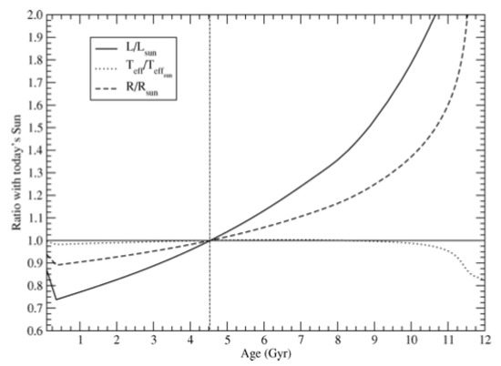
Figure 1. Evolution of the radius (effective temperature, and luminosity) of the Sun from the zero-age main sequence to the start of its red giant phase (cf. [9]).

This is practical evidence that $r_0/\widehat{R}<<1$. In particular, $r/\widehat{R}\le r_0/\widehat{R}<1$, so that $\mathrm{sign}$$\left[P_0\left(r\right)\right]=-1$; hence,

$$J_0\left(r\right)=\int \frac{rdr}{{\left({\widehat{R}}^2-r^2\right)}^{3/2}}=\frac{1}{\sqrt{{\widehat{R}}^2-r^2}}=\frac{1}{\widehat{R}}{\left(1-\frac{r^2}{{\widehat{R}}^2}\right)}^{-1/2},$$

$$\sqrt{\frac{\left|P_0\left(r\right)\right|}{r}}=\widehat{R}{\left(1-\frac{r^2}{{\widehat{R}}^2}\right)}^{1/2},{ϵ}_0=-1,$$

and (43)–(74) become (for $a=0$)

$$A=\frac{3}{2}{\left(1-\frac{r_0^2}{{\widehat{R}}^2}\right)}^{1/2},B{\widehat{R}}^2=\frac{1}{2},$$

(agreeing with (9.154) in [10] (p. 290)). Moreover,

$$F_0\left(r\right)=3\mathrm{sign}\left[P_0\left(r\right)\right]J_0\left(r\right)=-\frac{3}{\widehat{R}}{\left(1-\frac{r^2}{{\widehat{R}}^2}\right)}^{-1/2}$$

hence,

$$g_{00}=\frac{1}{4}\left(1-\frac{2m}{r_0}\right)\frac{\left|P_0\left(r\right)\right|}{r}{\left[F_0\left(r\right)-F_0\left(r_0\right)-2\sqrt{\frac{r_0}{\left|P_0\left(r_0\right)\right|}}\right]}^2={\left[\frac{1}{2}\sqrt{1-\frac{r^2}{{\widehat{R}}^2}}-\frac{3}{2}\sqrt{1-\frac{r_0^2}{{\widehat{R}}^2}}\right]}^2$$

(agreeing with (9.156) in [10] (p. 290)).

One has (with a satisfying (38))

$$-g_{11}={\left[1-\frac{r^2}{{\widehat{R}}^2}+\frac{r_0}{r}\left(\frac{r_0^2}{{\widehat{R}}^2}-\frac{2m}{r_0}\right)\right]}^{-1},P_a\left(r\right)=r^3-r_0^3-{\widehat{R}}^2\left(r-2m\right),$$

hence

$$g_{11}=\frac{{\widehat{R}}^{2}r}{P_a\left(r\right)}.$$

(47)

In particular, $g_a$ is only defined in (a region contained in) $P_a\left(r\right)<0$ (and $P_a\left(r_0\right)=-{\widehat{R}}^2\left(r_0-2m\right)<0$ because of $g_{00}>0$ for any $r\ge r_0$ for the exterior Schwarzschild solution), so that

$$F_a\left(r\right)-F_a\left(r_0\right)-2\sqrt{\frac{r_0}{\left|P_a\left(r_0\right)\right|}}=3\left\{J_a\left(r_0\right)-J_a\left(r\right)\right\}-\frac{2}{\widehat{R}}{\left(1-\frac{2m}{r_0}\right)}^{-1/2},$$

(48)

$$J_a\left(r_0\right)-J_a\left(r\right)={\int }_r^{r_0}\frac{s^{5/2}ds}{{\left(r_0^3-s^3+{\widehat{R}}^{2}s-2m{\widehat{R}}^2\right)}^{3/2}},$$

hence (the $g_{00}$ coefficient of $g_a$),

$$g_{00}=\frac{1}{4}\left(\frac{2m}{r_0}-1\right)\frac{P_a\left(r\right)}{r}{\left[\frac{2}{\widehat{R}}{\left(1-\frac{2m}{r_0}\right)}^{-1/2}+{\int }_{r_0}^r\frac{3s^{5/2}ds}{{\left(r_0^3-2m{\widehat{R}}^2+{\widehat{R}}^{2}s-s^3\right)}^{3/2}}\right]}^2,$$

(49)

where ${\widehat{R}}^2=r_0^3/\left(a+2m\right)$. The hyperelliptic integral in (49) may be derived from the integral in (60), thought of as a parametric integral

$$\frac{\partial }{\partial m}\int \frac{r^{5/2}dr}{\sqrt{r_0^3-r^3+{\widehat{R}}^2\left(r-2m\right)}}={\widehat{R}}^2\int \frac{r^{5/2}dr}{{\left(r_0^3-2m{\widehat{R}}^2+{\widehat{R}}^{2}r-r^3\right)}^{3/2}}$$

while the calculation of the antiderivative in (60) is addressed in Appendix A.

2. Pressure Field

To fully solve the boundary value problem (13)–(16), one is left with the determination of pressure field $p\left(r\right)$. To this end, we recall (24), implying (by $p\left(r\right)\ge 0$ and $\rho >0$) that $D>0$. Yet $D=\left(2/{\widehat{R}}^2\right)A$ or (by (43))

$$D=-\frac{3{ϵ}_a}{{\widehat{R}}^2}{\left(1-\frac{2m}{r_0}\right)}^{1/2}$$

(50)

yielding ${ϵ}_a=-1$. Note that (by (6) and (39)) ${\displaystyle P_a\left(r_0\right)=\frac{2m-r_0}{a+2m}{r}_0^3<0}$ hence,

$$-1={ϵ}_a=\mathrm{sign}\left\{2-3\sqrt{-\frac{P_a\left(r_0\right)}{r_0}}\right\}$$

or

$$a+2m<\frac{9r_0^2}{4}\left(r_0-2m\right).$$

(51)

As a consequence of (40), $\rho ={\rho }_a$ where

$${\rho }_a=\frac{3}{4\pi r_0^3}\left(M+\frac{c^2}{2\kappa }a\right).$$

(52)

Let us substitute from (52), (50) (with ${ϵ}_a=-1$) and (59) into (24). We obtain $p=p_a$ where

$$\frac{p_a}{c^2}+{\rho }_0+\frac{3c^2}{8\kappa \pi r_0^3}a=-\frac{2}{C{\widehat{R}}^2}\frac{{\displaystyle \sqrt{\frac{r}{\left|P_a\left(r\right)\right|}}}}{|v\left(a\right)-I_a\left(r\right)|}$$

(53)

where we set

$$I_a\left(r\right)={\int }_r^{r_0}\frac{s^{5/2}ds}{{\left[r_0^3-s^3+{\widehat{R}}^2\left(s-2m\right)\right]}^{3/2}},0\le r\le r_0.$$

(54)

$$v\left(a\right)=\frac{2}{3\widehat{R}}{\left(1-\frac{2m}{r_0}\right)}^{-1/2},a>-2m.$$

(55)

For $a=0$, Formula (53) becomes

$$\frac{p_0}{c^2}+{\rho }_0=2{\rho }_0|3-\frac{1}{r_0}{\left(\frac{r_0}{2m}-1\right)}^{-1/2}{\left(\frac{r_0^3}{2m}-r^2\right)}^{1/2}{|}^{-1}$$

(expressing the pressure field in the case considered by K. Schwarzschild, cf. op. cit.) (see Figure 2). We prove the following theorem: the following statements are equivalent: (i) $r_0>9m/4$ and (ii) there is an open neighbourhood of the origin $U_0\subset (-2m,+\infty )$, such that, for any $a\in U_0$, pressure field $p_a\left(r\right)$ is a bounded function in the interval $0\le r\le r_0$. With notations (54) and (55), pressure $p_a$ is bounded in $\left[0,r_0\right]$ if and only if $I_a\left(r\right)\ne v\left(a\right)$ for any $0\le r\le r_0$. We first attack the implication (ii) ⟹ (i). In particular (under Hypothesis (ii)), $p_0$ is bounded in $[0,r_0]$, yielding

$$I_0\left(r\right)-v\left(0\right)\ne 0,\forall 0\le r\le r_0,$$

(56)

where ${\displaystyle v\left(0\right)=\frac{2}{3}{\left(\frac{r_0^3}{2m}-r_0^2\right)}^{-1/2}}$ hence (56) is equivalent to

$$r^2+\frac{4r_0^3}{m}-9r_0^2\ne 0,\forall 0\le r\le r_0$$

so that it must be $9r_0^2-4r_0^3/m<0$ or

$$r_0>\frac{9m}{4}$$

(57)

which is (i). This is precisely the requirement (on structural parameters $r_0$ and M) discovered by K. Schwarzschild (cf. op. cit., or formula (9.163) in [10] (p. 292)) that ought to hold in order that pressure $p_0\left(r\right)$ may never become infinite inside the fluid.

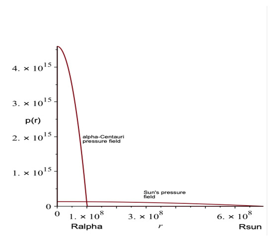
Figure 2. Pressure fields $p_{\odot }$ and $p_{\alpha -\mathrm{Centauri}}$ (Schwarzschild’s solution i.e., $a=0$).

To prove the implication (i) ⟹ (ii) is to show that the previous result persists under a small 1-parameter variation of $p_0$ about $a=0$. Let us assume that requirement (57) is satisfied. Then, (56) holds, so that (as $I_0\left(r\right)$ is strictly decreasing in $0\le r\le r_0$)one has $I_0\left(0\right)<v\left(0\right)$. Let us consider auxiliary function $\psi \left(a\right)=I_a\left(0\right)-v\left(a\right)$ defined in $a>-2m$. By the continuity of $\psi$, property $\psi \left(0\right)<0$ persists in some open neighbourhood $0\in U_0\subset (-2m,+\infty )$ i.e., $\psi \left(a\right)<0$ or $I_a\left(0\right)<v\left(a\right)$ for any $a\in U_0$. Lastly, as $I_a$ is strictly decreasing in $\left[0,r_0\right]$, we may conclude that

$$\forall a\in U_0,\forall 0\le r\le r_0:I_a\left(r\right)<v\left(a\right).$$

Q.e.d. As a corollary, we may show that the maximum domain $\mathsf{\Omega }\subset {\mathbb{R}}^4$ of the “physical” solution $\left(g_a,{\rho }_a,p_a\right)$ (obeying to the requirements ${\rho }_a\left(r\right)\ge 0$, $p_a\left(r\right)\ge 0$, and $p_a\left(r\right)$ is bounded in $0\le r\le r_0$)is $\mathsf{\Omega }=\mathbb{R}\times B_{r_0}\left(0\right)$, for any $a\in U_0$. Here $B_r\left(\mathbf{x}\right)$ denotes the closed ball of radius $r>0$ and center $\mathbf{x}\in {\mathbb{R}}^3$.

Indeed, as $g_{00}>0$ and $g_{11}<0$ in $\mathsf{\Omega }$, the domain is determined by the requirements $r\ne 0$, $P_a\left(r\right)<0$ and $I_a\left(r\right)\ne v\left(a\right)$. To compute $\mathsf{\Omega }$, note first that $P_a^{\prime }\left(r\right)=3r^2-r_0^3/\left(a+2m\right)$ and

$$\mathrm{Crit}\left(P_a\right)\cap \left[0,r_0\right]=\left\{\begin{array}{cc}\varnothing \hfill & {\displaystyle \mathrm{if}a+2m<\frac{r_0}{3},}\hfill \\ \\ {\displaystyle \sqrt{\frac{r_0^3}{3(a+2m)}}}\hfill & {\displaystyle \mathrm{if}a+2m\ge \frac{r_0}{3}.}\hfill \end{array}\right.$$

Consequently, if i) $a\ge 0$ then $P_a\left(r\right)<0$ for any $r\in \left[0,r_0\right]$, while if ii) $-2m<a<0$, there is a unique $r\left(a\right)\in \left(0,r_0\right)$ such that $P_a\left[r\left(a\right)\right]=0$, $P_a\left(r\right)>0$ for any $r\in \left[0,r\left(a\right)\right)$, and $P_a\left(r\right)<0$ for any $r\in \left(r\left(a\right),r_0\right]$.

3. Volume Calculations

The “true” physical density is not constant as an effect of curvature i.e., the metric $g_a$ (with $a=r_0^3/{\widehat{R}}^2-2m$) varies in the fluid ambient, and the very notion of density depends on $g_a$. To compute the “physical” density, let us set $d{s}_r=\sqrt{-g_{11}}dr$ (the “physically meaningful” radial interval), i.e.,

$$d{s}_r=\frac{\widehat{R}{r}^{1/2}}{\sqrt{r_0^3-r^3+{\widehat{R}}^2\left(r-2m\right)}}dr.$$

(58)

Similarly, $d{s}_{\theta }=\sqrt{-g_{22}}d\theta =rd\theta$ and $d{s}_{\phi }=\sqrt{-g_{33}}d\phi =rsin\theta d\phi$. The “physical” volume element is then

$$dV=d{s}_{r}d{s}_{\theta }d{s}_{\phi }=\frac{\widehat{R}{r}^{5/2}sin\theta }{\sqrt{r_0^3-r^3+{\widehat{R}}^2\left(r-2m\right)}}drd\theta d\phi .$$

(59)

Let us integrate in (59) over $0\le \theta \le \pi$, $0\le \phi \le 2\pi$ and $0\le r\le r_0$ so that to determine the total volume

$$V={\int }_0^{\pi }d\theta {\int }_0^{2\pi }d\phi {\int }_0^{r_0}\frac{\widehat{R}{r}^{5/2}sin\theta dr}{\sqrt{r_0^3-r^3+{\widehat{R}}^2\left(r-2m\right)}}=4\pi \widehat{R}{\int }_0^{r_0}\frac{r^{5/2}dr}{\sqrt{r_0^3-r^3+{\widehat{R}}^2\left(r-2m\right)}}.$$

(60)

To compute V, we rely on considerations in Appendix A (reducing the underlying indefinite integral to the canonical Legendre form). Let us assume that

$$a>\frac{2}{3\sqrt{3}}\widehat{R},\sigma >0,\tau <{\sigma }^2<4\tau ,$$

(61)

(yielding $\mathbf{m}=-h^2<0$, ${\mathbf{m}}^{\prime }={h^{\prime }}^2>0$ and $\mathcal{A}<0$, with the notations in Appendix A). The first of the assumptions (61) yields $a>0$, and (61) is then equivalent to $a>a_0$, where $a_0\in \mathbb{R}$ is the only positive root of the polynomial ${\displaystyle F\left(X\right)=X^3+2m{X}^2-\frac{4r_0^3}{27}\in \mathbb{R}\left[X\right]}$. Indeed (by the boundary condition (38))$a^2>4{\widehat{R}}^2/27$ is equivalent (for positive a) to $F\left(a\right)>0$. Yet, $F\left(0\right)<0$, F is monotonously increasing in $(0,+\infty )$, and ${lim}_{X\to +\infty }F\left(X\right)=+\infty$ hence there is a unique $a_0>0$, such that $F\left(a_0\right)=0$. Lastly, the last two requirements in (61) are satisfied for every $a>a_0$. Next, note that

$$\mu <r_0.$$

(62)

Indeed, starting from ${\displaystyle \mu =\frac{1}{2\sigma }\left[-\tau +\sqrt{\tau (\tau +2{\sigma }^2)}\right]}$ inequality (62) is equivalent to $\tau \sigma <2r_0(\tau +r_0\sigma )$ or (by replacing $\tau$ from $\sigma \tau =r_0^3-2m{\widehat{R}}^2$)$Q\left(\sigma \right)>0$ where ${\displaystyle Q\left(x\right)=\frac{2r_0^2}{r_0^3-2m{\widehat{R}}^2}{x}^2-x+2r_0}$. Yet $Q\left(x\right)>0$ for any $x\in \mathbb{R}$. Q.e.d.

Let us set

$$g\left(x\right)=\frac{x^{5/2}}{\sqrt{r_0^3-x^3+{\widehat{R}}^2\left(x-2m\right)}},x^3-{\widehat{R}}^{2}x+2m{\widehat{R}}^2-r_0^3<0.$$

The domain of g is $(-\infty ,\sigma )$ (cf. Table A1).Note that

$$r_0<\sigma$$

(63)

(hence, integral in (60) is well-defined).To prove (63) one observes first that

$$r_0<\sigma ⟺2m<\sigma ⟹r_0^2-{\widehat{R}}^2<\tau .$$

(64)

The remainder of the argument is by contradiction. If $r_0\ge \sigma$, then (by (64))$\sigma \tau \ge 2m\left(r_0^2-{\widehat{R}}^2\right)$ or [again by $\sigma \tau =r_0^3-2m{\widehat{R}}^2$] $2m\ge r_0$ [in contradiction with ${\left(g_S\right)}_{00}>0$]. As a corollary to (63)

$$\frac{1}{h^2}={\left(\frac{\nu }{\mu }\right)}^2<t_o^2.$$

(65)

where $t_o=\left(\nu -r_0\right)/\left(r_0-\mu \right)$. Indeed

$${\left(\frac{\nu }{\mu }\right)}^2<{\left(\frac{\nu -r_0}{r_0-\mu }\right)}^2⟺r_0\left({\nu }^2-{\mu }^2\right)+2\mu \nu \left(\mu -\nu \right)<0⟺\left(63\right)$$

[by substitution from ${\displaystyle \mu \nu =-\frac{\tau }{2}}$, ${\displaystyle \mu -\nu =\frac{1}{\sigma }\sqrt{\tau \left(\tau +2{\sigma }^2\right)}}$ and ${\displaystyle {\nu }^2-{\mu }^2=\frac{\tau }{{\sigma }^2}\sqrt{\tau \left(\tau +2{\sigma }^2\right)}}$]. As part of the reduction to the canonical form scheme one needs to apply a homographic change of variables $x=\left(\mu t+\nu \right){\left(t+1\right)}^{-1}$ under the integral sign. Yet the pre-images $\left\{-\nu /\mu ,t_o\right\}$ of $\left\{0,r_0\right\}$ are separated by the singularity $t=-1$; hence, one needs to split (by taking into account (62))integral ${\int }_0^{r_0}g\left(x\right)dx$ as ${\int }_0^{\mu }g\left(x\right)dx+{\int }_{\mu }^{r_0}g\left(x\right)dx$ and apply the transformations $x:\left(-1,+\infty \right)\to \left(-\infty ,\mu \right)$ and $x:\left(-\infty ,-1\right)\to \left(\mu ,+\infty \right)$, respectively. This leads to generalized integrals, so a bit of extra pedantry is needed to correctly apply change of variable theorems, i.e.,

$${\int }_0^{r_0}g\left(x\right)dx=\underset{\begin{array}{c}\alpha \to 0^{+}\\ \beta \to {\mu }^{-}\end{array}}{lim}{\int }_{\alpha }^{\beta }g\left(x\right)dx+\underset{\begin{array}{c}\alpha \to {\mu }^{+}\\ \beta \to r_0^{-}\end{array}}{lim}{\int }_{\alpha }^{\beta }g\left(x\right)dx=\underset{\begin{array}{c}\alpha \to 0^{+}\\ \beta \to {\mu }^{-}\end{array}}{lim}{I}_{\alpha \beta }+\underset{\begin{array}{c}\alpha \to {\mu }^{+}\\ \beta \to r_0^{-}\end{array}}{lim}{I}_{\alpha \beta }$$

where

$$I_{\alpha \beta }:={\int }_{t_{\alpha }}^{t_{\beta }}\frac{{\mathcal{R}}^{*}\left(t\right)dt}{\sqrt{\mathcal{A}\left(1-h^2{t}^2\right)\left(1+{h^{\prime }}^2{t}^2\right)}}$$

with A) $1<-\nu /\mu <t_{\alpha }<t_{\beta }$, respectively, B) $t_{\alpha }<t_{\beta }<t_{r_0}<-1$. Here, $t_{\gamma }:=\left(\nu -\gamma \right){\left(\gamma -\mu \right)}^{-1}$ [so that $t_o=t_{r_0}$]. Next, one decomposes ${\mathcal{R}}^{*}$ into even and odd components, i.e., ${\mathcal{R}}^{*}\left(t\right)={\mathcal{R}}_1\left(t^2\right)+t{\mathcal{R}}_2\left(t^2\right)$; hence, (in Case (A))

$$\underset{\begin{array}{c}\alpha \to 0^{+}\\ \beta \to {\mu }^{-}\end{array}}{lim}{I}_{\alpha \beta }=\underset{\begin{array}{c}\alpha \to 0^{+}\\ \beta \to {\mu }^{-}\end{array}}{lim}{\int }_{t_{\alpha }}^{t_{\beta }}\frac{\left[{\mathcal{R}}_1\left(t^2\right)+t{\mathcal{R}}_2\left(t^2\right)\right]dt}{\sqrt{\mathcal{A}\left(1-h^2{t}^2\right)\left(1+{h^{\prime }}^2{t}^2\right)}}=$$

(by $ht={\left(1-z^2\right)}^{-1/2}$ with $0<z<1$)

$$=\underset{\begin{array}{c}\alpha \to 0^{+}\\ \beta \to {\mu }^{-}\end{array}}{lim}\left\{\frac{k\left(\mu +\nu \right)}{h\sqrt{-\mathcal{A}}}{\int }_{z_{\alpha }}^{z_{\beta }}\frac{{\mathcal{R}}_1^{*}\left(z^2\right)dz}{\sqrt{\left(1-z^2\right)\left(1-k^2{z}^2\right)}}+{\left.\mathcal{S}\left[\frac{1}{h^2\left(1-z^2\right)}\right]\right|}_{z_{\alpha }}^{z_{\beta }}\right\}=$$

(where $z_{\alpha }=\sqrt{1-1/\left(h^2{t}_{\alpha }^2\right)}$] or [by $z=sin\varphi$, $0<\varphi <\pi /2$)

$$=\underset{\begin{array}{c}\alpha \to 0^{+}\\ \beta \to {\mu }^{-}\end{array}}{lim}\left\{\frac{k\left(\mu +\nu \right){\nu }^2}{h{\mathcal{M}}^{\prime }\sqrt{-\mathcal{A}}}[8k^{2}cot\varphi \sqrt{1-k^2{sin}^2\varphi }{|}_{{\varphi }_{\alpha }}^{{\varphi }_{\beta }}\right.$$

$$+\left(1-8k^2\right){\int }_{{\varphi }_{\alpha }}^{{\varphi }_{\beta }}\frac{d\varphi }{\sqrt{1-k^2{sin}^2\varphi }}+8k^2{\int }_{{\varphi }_{\alpha }}^{{\varphi }_{\beta }}\sqrt{1-k^2{sin}^2\varphi }d\varphi$$

$$\left.+\left[8k^2\left(1-k^2\right)-1\right]{\int }_{{\varphi }_{\alpha }}^{{\varphi }_{\beta }}\frac{d\varphi }{\left(1-k^2{sin}^2\varphi \right)\sqrt{1-k^2{sin}^2\varphi }}]+\mathcal{S}\left(\frac{1}{h^2{cos}^2\varphi }\right){|}_{{\varphi }_{\alpha }}^{{\varphi }_{\beta }}\right\}$$

(where ${\varphi }_{\alpha }=arcsin{z}_{\alpha }$) and

$$\underset{\begin{array}{c}\alpha \to 0^{+}\\ \beta \to {\mu }^{-}\end{array}}{lim}\left[\frac{8k^3\left(\mu +\nu \right){\nu }^2}{h{\mathcal{M}}^{\prime }\sqrt{-\mathcal{A}}}cot\varphi \sqrt{1-k^2{sin}^2\varphi }+\mathcal{S}\left(\frac{1}{h^2{cos}^2\varphi }\right)\right]{|}_{{\varphi }_{\alpha }}^{{\varphi }_{\beta }}$$

(by (A22))

$$=\frac{4k^3{\left(\mu +\nu \right)}^2\mu }{h^2\left(\nu -\mu \right)\left(2\mu +\nu \right)\sqrt{-\mathcal{A}}}\underset{\begin{array}{c}\alpha \to 0^{+}\\ \beta \to {\mu }^{-}\end{array}}{lim}F\left(\varphi \right){|}_{{\varphi }_{\alpha }}^{{\varphi }_{\beta }}=\frac{4k^3\left(3-4k^2\right)}{h^2\sqrt{1-k^2}}\frac{{\left(\mu +\nu \right)}^2\mu }{\left(\nu -\mu \right)\left(2\mu +\nu \right)\sqrt{-\mathcal{A}}}$$

where

$$F\left(\varphi \right):=\frac{1}{sin\varphi }\left[\frac{2+\left(1-4k^2\right){sin}^2\varphi }{\sqrt{1-k^2{sin}^2\varphi }}-2cos\varphi \sqrt{1-k^2{sin}^2\varphi }\right].$$

Indeed, $\alpha \to 0^{+}$, $\beta \to {\mu }^{-}⟹{\varphi }_{\alpha }\to 0^{+}$, ${\displaystyle {\varphi }_{\beta }\to {\left(\frac{\pi }{2}\right)}^{-}}$ and

$$\underset{\varphi \to 0}{lim}F\left(\varphi \right)=0,\underset{\varphi \to \frac{\pi }{2}}{lim}F\left(\varphi \right)=\frac{3-4k^2}{\sqrt{1-k^2}}.$$

Lastly, (in Case (A))

$$\underset{\begin{array}{c}\alpha \to 0^{+}\\ \beta \to {\mu }^{-}\end{array}}{lim}{I}_{\alpha \beta }=\frac{4k^3\left(3-4k^2\right)}{h^2\sqrt{1-k^2}}\frac{{\left(\mu +\nu \right)}^2\mu }{\left(\nu -\mu \right)\left(2\mu +\nu \right)\sqrt{-\mathcal{A}}}$$

$$+\frac{k\nu {\left(\mu +\nu \right)}^2}{h\left(\nu -\mu \right)\left(2\mu +\nu \right)\sqrt{-\mathcal{A}}}[\left(1-8k^2\right){\int }_0^{\pi /2}\frac{d\varphi }{\sqrt{1-k^2{sin}^2\varphi }}+8k^2{\int }_0^{\pi /2}\sqrt{1-k^2{sin}^2\varphi }d\varphi$$

$$+\left[8k^2\left(1-k^2\right)-1\right]{\int }_0^{\pi /2}\frac{d\varphi }{\left(1-k^2{sin}^2\varphi \right)\sqrt{1-k^2{sin}^2\varphi }}]$$

or

$$\underset{\begin{array}{c}\alpha \to 0^{+}\\ \beta \to {\mu }^{-}\end{array}}{lim}{I}_{\alpha \beta }=\frac{k\nu {\left(\mu +\nu \right)}^2}{h\left(\nu -\mu \right)\left(2\mu +\nu \right)\sqrt{-\mathcal{A}}}\times$$

(66)

$$\times \left\{\left(1-8k^2\right)\mathbf{F}\left(k,\frac{\pi }{2}\right)+8k^2\mathbf{E}\left(k,\frac{\pi }{2}\right)+\left[8k^2\left(1-k^2\right)-1\right]\Pi \left(k^2,k\right)+\frac{4k^2\left(4k^2-3\right)}{\sqrt{1-k^2}}\right\}$$

with the Legendre notations

$$\mathbf{F}\left(k,\theta \right)={\int }_0^{\theta }\frac{d\varphi }{\sqrt{1-k^2{sin}^2\varphi }},\mathbf{E}\left(k,\theta \right)={\int }_0^{\theta }\sqrt{1-k^2{sin}^2\varphi }d\varphi ,$$

$$\Pi \left(\ell ,k\right)={\int }_0^{\pi /2}\frac{d\varphi }{\left(1-\ell {sin}^2\varphi \right)\sqrt{1-k^2{sin}^2\varphi }},$$

for the abelian integrals of the first, second, and third kind of module k. As to Case (B),

$$\underset{\begin{array}{c}\alpha \to {\mu }^{+}\\ \beta \to r_0^{-}\end{array}}{lim}{I}_{\alpha \beta }=\underset{\begin{array}{c}\alpha \to {\mu }^{+}\\ \beta \to r_0^{-}\end{array}}{lim}{\int }_{t_{\alpha }}^{t_{\beta }}\frac{{\mathcal{R}}^{*}\left(t\right)dt}{\sqrt{\mathcal{A}\left(1-h^2{t}^2\right)\left(1+{h^{\prime }}^2{t}^2\right)}}=$$

[by setting $s=-t]$

$$=\underset{\begin{array}{c}\alpha \to {\mu }^{+}\\ \beta \to r_0^{-}\end{array}}{lim}\left[{\int }_{-t_{\beta }}^{-t_{\alpha }}\frac{{\mathcal{R}}_1\left(t^2\right)dt}{\sqrt{\mathcal{A}\left(1-h^2{t}^2\right)\left(1+{h^{\prime }}^2{t}^2\right)}}-{\int }_{-t_{\beta }}^{-t_{\alpha }}\frac{t{\mathcal{R}}_2\left(t^2\right)dt}{\sqrt{\mathcal{A}\left(1-h^2{t}^2\right)\left(1+{h^{\prime }}^2{t}^2\right)}}\right]=$$

[with ${\displaystyle -t_{\alpha }>-t_{\beta }>-t_{r_0}>\frac{1}{h}]}$ or [by $ht={\left(1-z^2\right)}^{-1/2}$, $0<z<1$]

$$=\underset{\begin{array}{c}\alpha \to {\mu }^{+}\\ \beta \to r_0^{-}\end{array}}{lim}\left[-\frac{\left(\mu +\nu \right)k}{h\sqrt{-\mathcal{A}}}{\int }_{z_{\alpha }}^{z_{\beta }}\frac{{\mathcal{R}}_1^{*}\left(z^2\right)dz}{\sqrt{\left(1-z^2\right)\left(1-k^2{z}^2\right)}}+\mathcal{S}\left(\frac{1}{h^2\left(1-z^2\right)}\right){|}_{z_{\alpha }}^{z_{\beta }}\right]$$

$$=\underset{\begin{array}{c}\alpha \to {\mu }^{+}\\ \beta \to r_0^{-}\end{array}}{lim}\left\{-\frac{k\left(\mu +\nu \right){\nu }^2}{h{\mathcal{M}}^{\prime }\sqrt{-\mathcal{A}}}[8k^{2}cot\varphi \sqrt{1-k^2{sin}^2\varphi }{|}_{{\varphi }_{\alpha }}^{{\varphi }_{\beta }}\right.$$

$$+\left(1-8k^2\right){\int }_{{\varphi }_{\alpha }}^{{\varphi }_{\beta }}\frac{d\varphi }{\sqrt{1-k^2{sin}^2\varphi }}+8k^2{\int }_{{\varphi }_{\alpha }}^{{\varphi }_{\beta }}\sqrt{1-k^2{sin}^2\varphi }d\varphi$$

$$\left.+\left[8k^2\left(1-k^2\right)-1\right]{\int }_{{\varphi }_{\alpha }}^{{\varphi }_{\beta }}\frac{d\varphi }{\left(1-k^2{sin}^2\varphi \right)\sqrt{1-k^2{sin}^2\varphi }}]+\mathcal{S}\left(\frac{1}{h^2{cos}^2\varphi }\right){|}_{{\varphi }_{\alpha }}^{{\varphi }_{\beta }}\right\}.$$

Note that ${\displaystyle \alpha \to {\mu }^{+}⟹{\varphi }_{\alpha }=arcsin\sqrt{1-\frac{1}{h^2}{\left(\frac{\alpha -\mu }{\nu -\alpha }\right)}^2}\to \frac{\pi }{2}}$ and ${\displaystyle \beta \to r_0^{-}⟹{\varphi }_{\beta }=arcsin\sqrt{1-\frac{1}{h^2}{\left(\frac{\beta -\mu }{\nu -\beta }\right)}^2}\to arcsin\sqrt{1-\frac{1}{h^2{t}_o^2}}=:{\varphi }_o}$. Summing up our previous calculations

$$\mathcal{S}\left(\frac{1}{h^2{cos}^2\varphi }\right)=\frac{4k^3\mu {\left(\mu +\nu \right)}^2}{h^2\left(\nu -\mu \right)\left(2\mu +\nu \right)\sqrt{-\mathcal{A}}}\frac{2+\left(1-4k^2\right){sin}^2\varphi }{sin\varphi \sqrt{1-k^2{sin}^2\varphi }};$$

hence,

$$\underset{\begin{array}{c}\alpha \to {\mu }^{+}\\ \beta \to r_0^{-}\end{array}}{lim}\left\{-\frac{8k^3\left(\mu +\nu \right){\nu }^2}{h{\mathcal{M}}^{\prime }\sqrt{-\mathcal{A}}}cot\varphi \sqrt{1-k^2{sin}^2\varphi }+\mathcal{S}\left(\frac{1}{h^2{cos}^2\varphi }\right)\right\}{|}_{{\varphi }_{\alpha }}^{{\varphi }_{\beta }}$$

$$=\frac{4k^3\mu {\left(\mu +\nu \right)}^2}{h^2\left(\nu -\mu \right)\left(2\mu +\nu \right)\sqrt{-\mathcal{A}}}\left[G\left({\varphi }_o\right)+\frac{4k^2-3}{\sqrt{1-k^2}}\right]$$

where

$$G\left(\varphi \right):=\frac{1}{sin\varphi }\left[\frac{2+\left(1-4k^2\right){sin}^2\varphi }{\sqrt{1-k^2{sin}^2\varphi }}+2cos\varphi \sqrt{1-k^2{sin}^2\varphi }\right].$$

Thus,

$$\underset{\begin{array}{c}\alpha \to {\mu }^{+}\\ \beta \to r_0^{-}\end{array}}{lim}{I}_{\alpha \beta }=\frac{k{\left(\mu +\nu \right)}^2\nu }{h\left(\nu -\mu \right)\left(2\mu +\nu \right)\sqrt{-\mathcal{A}}}\times$$

$$\times [\left(1-8k^2\right){\int }_{{\varphi }_o}^{\pi /2}\frac{d\varphi }{\sqrt{1-k^2{sin}^2\varphi }}+8k^2{\int }_{{\varphi }_o}^{\pi /2}\sqrt{1-k^2{sin}^2\varphi }d\varphi$$

$$+\left[8k^2\left(1-k^2\right)-1\right]{\int }_{{\varphi }_o}^{\pi /2}\frac{d\varphi }{\left(1-k^2{sin}^2\varphi \right)\sqrt{1-k^2{sin}^2\varphi }}]$$

$$+\frac{4k^3\mu {\left(\mu +\nu \right)}^2}{h^2\left(\nu -\mu \right)\left(2\mu +\nu \right)\sqrt{-\mathcal{A}}}\left[G\left({\varphi }_o\right)+\frac{4k^2-3}{\sqrt{1-k^2}}\right]$$

and

$$G\left({\varphi }_o\right)=\frac{1}{\sqrt{h^2{t}_o^2-1}}\left[\frac{\left(3-4k^2\right)h^2{t}_o^2+4k^2-1}{\sqrt{k^2+\left(1-k^2\right)h^2{t}_o^2}}-\frac{2}{h{t}_o}\sqrt{k^2+\left(1-k^2\right)h^2{t}_o^2}\right].$$

(67)

Then (in Case (B))

$$\underset{\begin{array}{c}\alpha \to {\mu }^{+}\\ \beta \to r_0^{-}\end{array}}{lim}{I}_{\alpha \beta }=\frac{k{\left(\mu +\nu \right)}^2\nu }{h\left(\nu -\mu \right)\left(2\mu +\nu \right)\sqrt{-\mathcal{A}}}\times$$

(68)

$$\times \{\left(1-8k^2\right)\left[\mathbf{F}\left(k,\frac{\pi }{2}\right)-\mathbf{F}\left(k,{\varphi }_o\right)\right]+8k^2\left[\mathbf{E}\left(k,\frac{\pi }{2}\right)-\mathbf{E}\left(k,{\varphi }_0\right)\right]$$

$$+\left[8k^2\left(1-k^2\right)-1\right]\left[\Pi \left(k^2,k\right)-{\int }_0^{{\varphi }_0}\frac{d\varphi }{\left(1-k^2{sin}^2\varphi \right)\sqrt{1-k^2{sin}^2\varphi }}\right]\}$$

$$+\frac{4k^3\mu {\left(\mu +\nu \right)}^2}{h^2\left(\nu -\mu \right)\left(2\mu +\nu \right)\sqrt{-\mathcal{A}}}\left[G\left({\varphi }_o\right)+\frac{4k^2-3}{\sqrt{1-k^2}}\right].$$

Summing up (by (66)–(68))

$${\int }_0^{r_0}g\left(x\right)dx=\frac{k{\left(\mu +\nu \right)}^2\nu }{h\left(\nu -\mu \right)\left(2\mu +\nu \right)\sqrt{-\mathcal{A}}}\times$$

(69)

$$\times \{\left(1-8k^2\right)\left[2\mathbf{F}\left(k,\frac{\pi }{2}\right)-\mathbf{F}\left(k,{\varphi }_o\right)\right]+8k^2\left[2\mathbf{E}\left(k,\frac{\pi }{2}\right)-\mathbf{E}\left(k,{\varphi }_0\right)\right]$$

$$+\left[8k^2\left(1-k^2\right)-1\right]\left[2\Pi \left(k^2,k\right)-{\int }_0^{{\varphi }_0}\frac{d\varphi }{\left(1-k^2{sin}^2\varphi \right)\sqrt{1-k^2{sin}^2\varphi }}\right]\}$$

$$+\frac{4k^3\mu {\left(\mu +\nu \right)}^2}{h^2\left(\nu -\mu \right)\left(2\mu +\nu \right)\sqrt{-\mathcal{A}}}\frac{1}{\sqrt{h^2{t}_o^2-1}}\left[\frac{\left(3-4k^2\right)h^2{t}_o^2+4k^2-1}{\sqrt{k^2+\left(1-k^2\right)h^2{t}_o^2}}-\frac{2}{h{t}_o}\sqrt{k^2+\left(1-k^2\right)h^2{t}_o^2}\right].$$

Going back to (60), volume $V\left(a\right)$ of region $0\le r\le r_0$, whose geometry is governed by $g_a$, is

$$V\left(a\right)=4\pi \widehat{R}I\left(a\right),I\left(a\right):={\int }_0^{r_0}\frac{r^{5/2}dr}{\sqrt{{\displaystyle \frac{a+r}{a+2m}{r}_0^3-r^3}}}.$$

In particular, for $a=0$ [as (38) with $a=0$ yields ${\displaystyle {\widehat{R}}^2=\frac{r_0^3}{2m}]}$

$$V\left(0\right)=4\pi {\int }_0^{r_0}\frac{r^{2}dr}{{\displaystyle \sqrt{1-{\left(\frac{r}{\widehat{R}}\right)}^2}}}=2\pi {\widehat{R}}^{3}f\left(\frac{r_0}{\widehat{R}}\right),f\left(x\right)=arcsinx-x\sqrt{1-x^2},\left|x\right|\le 1.$$

This is the case examined by K. Schwarzschild (cf. op. cit.); practical evidence was previously gathered that $r_0/\widehat{R}<<1$; hence, we may consider the truncated Taylor expansion of $V\left(0\right)$ as a function of $r_0/\widehat{R}$, i.e., for every $n\in {\mathbb{Z}}_{+}$

$$V\left(0\right)=2\pi {\widehat{R}}^3\left[\sum _{k=0}^n{(-1)}^k{a}_k{\left(\frac{r_0}{\widehat{R}}\right)}^{2k+1}+R_{2n+2}\left(\frac{r_0}{\widehat{R}};0\right)\right],$$

$$a_k=\frac{1}{2k+1}\left(\begin{array}{c}-1/2\\ k\end{array}\right)-\left(\begin{array}{c}1/2\\ k\end{array}\right),0\le k\le n,$$

$$R_{2n+2}(x;0)={(-1)}^{n+1}\left\{\left(\begin{array}{c}-1/2\\ n+1\end{array}\right){\int }_0^x{t}^{2n+2}{\left[1-\eta {\left(t\right)}^2\right]}^{-n-1/2}\right.$$

$$\left.-\left(\begin{array}{c}1/2\\ n+1\end{array}\right)x^{2n+3}{\left[1-\eta {\left(x\right)}^2\right]}^{-n-1/2}\right\},$$

$$\left(\begin{array}{c}\alpha \\ 0\end{array}\right)=1,\left(\begin{array}{c}\alpha \\ k\end{array}\right)=\frac{\alpha (\alpha -1)\cdots (\alpha -k+1)}{k!},\alpha \in \mathbb{R},k\in \mathbb{N},$$

for some function $\eta :[-1,1]\to \mathbb{R}$ such that $\eta \left(x\right)$ lies between 0 and x, or

$$V\left(0\right)=\frac{4\pi r_0^3}{3}\left[1+\frac{3}{10}{\left(\frac{r_0}{\widehat{R}}\right)}^2+\frac{3}{2}\sum _{k=3}^n{(-1)}^k{a}_k{\left(\frac{r_0}{\widehat{R}}\right)}^{2(k-1)}+\frac{3}{2}{\left(\frac{r_0}{\widehat{R}}\right)}^{-3}{R}_{2n+2}\left(\frac{r_0}{\widehat{R}};0\right)\right]$$

(70)

and

$$\left|\frac{3}{2}{\left(\frac{r_0}{\widehat{R}}\right)}^{-3}{R}_{2n+2}\left(\frac{r_0}{\widehat{R}};0\right)\right|\le \frac{3\left(n+\frac{5}{4}\right)2^{n+\frac{1}{2}}}{(n+1)(2n+3)}{\left(\frac{r_0}{\widehat{R}}\right)}^{2n}.$$

(71)

Estimate (71) follows from

$$\left|R_{2n+2}\left(x;0\right)\right|\le \frac{n+\frac{5}{4}}{(n+1)(2n+3)}{\left(2x^2\right)}^{n+\frac{3}{2}},\left|x\right|<\frac{1}{\sqrt{2}}.$$

(72)

Indeed, if for instance $x>0$, then $0<\eta <x$ yields $1/\left(1-{\eta }^2\right)<1/2$; hence,

$$\left|{\int }_0^x{t}^{2n+2}{\left[1-\eta {\left(t\right)}^2\right]}^{-n-\frac{3}{2}}dt\right|\le \frac{{\left(2x^2\right)}^{n+\frac{3}{2}}}{2n+3}$$

(73)

and ${\displaystyle \left(\begin{array}{c}-1/2\\ n+1\end{array}\right)=\frac{{(-1)}^{n+1}}{2^{n+1}}\frac{(2n+1)!!}{(n+1)!}}$, so that

$$\left|\left(\begin{array}{c}-1/2\\ n+1\end{array}\right)\right|=\frac{3\times 5·\cdots ·(2n+1)}{2^{n+1}(n+1)!}\le \frac{4\times 6·\cdots ·(2n+2)}{2^{n+1}(n+1)!}=\frac{1}{2}$$

i.e.,

$$\left|\left(\begin{array}{c}-1/2\\ n+1\end{array}\right)\right|\le \frac{1}{2}.$$

(74)

Similarly,

$$\left|x^{2n+3}{\left[1-\eta {\left(x\right)}^2\right]}^{-n-\frac{1}{2}}\right|\le \frac{1}{2}{\left(2x^2\right)}^{n+\frac{3}{2}}$$

(75)

and ${\displaystyle \left(\begin{array}{c}1/2\\ n+1\end{array}\right)=\frac{{(-1)}^n}{2^{n+1}}\frac{(2n-1)!!}{(n+1)!}}$ so that

$$\left|\left(\begin{array}{c}1/2\\ n+1\end{array}\right)\right|\le \frac{1}{2(n+1)}.$$

(76)

Lastly, estimates (73)–(76) yield (72) for any $0<x<1/\sqrt{2}$. Of course, the use of (74) and (76) does not lead to an optimal estimate on $\left|R_{2n+2}(x;0)\right|$ ((72) is to be preferred only for its mathematical elegance).

4. Conclusions and Open Problems

In the present paper, we examined a fundamental issue, present in most textbooks nowadays on general relativity and gravitation theory, i.e., the derivation of the interior Schwarzschild solution $g_0$ (cf. e.g., [10] (pp. 280–295)) and the resulting simple model of a star. To determine $g_0$ (and actually $(g_0,{\rho }_0,p_0)$ where ${\rho }_0$ is the (constant) density and $p_0$ the (radial) pressure field), one looks for a line element $ds$ of the form $d{s}^2=e^{\nu \left(r\right)}{c}^{2}d{t}^2-\left[e^{\lambda \left(r\right)}d{r}^2+r^2\left(d{\theta }^2+{sin}^2\theta d{\phi }^2\right)\right]$ and needs to solve the boundary value problem (13)–(16) for $(\lambda ,\mu ,\rho ,p)$. The general solution of the ODE system (13)–(15) contains three constants of integration $A,B,a\in \mathbb{R}$, and the given boundary conditions determine the first two, while the third is but subject to the constraint $a>-2m$. This leads to a 1-parameter family of solutions ${\left\{\left({\lambda }_a,{\mu }_a,{\rho }_a,p_a\right)\right\}}_{a>-2m}$ to (13)–(16) with the property that ${\lambda }_a\left(r\right)$ is bounded at $r=0$ if and only if $a=0$. K. Schwarzschild discarded the solutions with $a\ne 0$ on the ground that the determinant of each $g_a$ with $a\ne 0$ vanishes at $r=0$; this is, of course, also the case for $g_0$, and the question arises whether any of the additional solutions $g_a$ is physically acceptable, thus leading to alternative geometric descriptions of the interior of a star of incompressible fluid. We explicitly determine the solutions ${\left\{\left(g_a,{\rho }_a,p_a\right)\right\}}_{a>-2m}$ and show that the requirement (57) i.e., $r_0>9m/4$, which in Schwarzschild’s work is equivalent to $p_0\left(r\right)$ staying finite in $r\le r_0$, is also equivalent to the boundedness of $p_a\left(r\right)$ in $r\le r_0$, though only for a lying in some open neighbourhood $U_0\subset (-2m,+\infty )$ of $a=0$. It should be observed that estimate (6) i.e., $r_0>2m$ is slightly improved by estimate (57); ${\displaystyle \left(6\right)⟺M<\frac{c^2{r}_0}{2\kappa }}$ and ${\displaystyle \left(57\right)⟺M<\frac{4}{9}\frac{c^2{r}_0}{2\kappa }}$, so that the requirement (57) provides a slightly smaller upper bound on the amount M of fluid that can be packed into a ball of radius $r_0$, in agreement with the geometry of space-time as described by the Lorentzian metric ${\displaystyle g=\left\{\begin{array}{cc}{g}_a\hfill & r\le r_0\hfill \\ g_S\hfill & r\ge r_0\hfill \end{array}\right.}$. K. Schwarzschild used metric tensor $g_0$ to compute the volume of the region $r\le r_0$

$$V\left(0\right)={\int }_0^{\pi }d\theta {\int }_0^{2\pi }d\phi {\int }_0^{r_0}\frac{r^{2}sin\theta dr}{{\displaystyle \sqrt{1-\frac{r^2}{{\widehat{R}}^2}}}}$$

and derived the truncated Taylor development of $V\left(0\right)$ with respect to the parameter $r_0/\widehat{R}$

$$V\left(0\right)=\frac{4\pi r_0^3}{3}\left[1+\frac{3}{10}{\left(\frac{r_0}{\widehat{R}}\right)}^2+O{\left(\frac{r_0}{\widehat{R}}\right)}^4\right].$$

(77)

When the geometry is described by $g_0$, the parameter $r_0/\widehat{R}$ is $<<1$, as may be argued by invoking experimental evidence, and development (77) gives a fair approximation to volume $V\left(0\right)$. We slightly improved Schwarzschild’s result by developing $V\left(0\right)$ to arbitrary fixed order (cf. our (70) in $\mathsf{\S }3$) and providing a mathematically elegant estimate on the Taylor rest (cf. (71) in $\mathsf{\S }3$)

$$\left|R_{2n+2}\left(\frac{r_0}{\widehat{R}};0\right)\right|\le \frac{\left(n+\frac{5}{4}\right)2^{n+\frac{3}{2}}}{(n+1)(2n+3)}{\left(\frac{r_0}{\widehat{R}}\right)}^{2n+3}.$$

On the basis of our discussion of the parameter $r_0/\widehat{R}$ in $\mathsf{\S }1$ for the Sun, one has $r_0/\widehat{R}<<1$ beyond Sun’s present age, and Formulas (70) and (71) remain accurate up to the start of Sun’s red giant phase. The calculation of the volume

$$V\left(a\right)={\int }_0^{\pi }d\theta {\int }_0^{2\pi }d\phi {\int }_0^{r_0}\frac{\widehat{R}{r}^{5/2}sin\theta dr}{\sqrt{r_0^3-r^3+{\widehat{R}}^2\left(r-2m\right)}}$$

turned out to be more involved, as depending upon the evaluation of an abelian integral that may not be expressed in terms of algebraic functions, and which we can only reduce to the canonical Legendre form (cf. (60) and (69) in $\mathsf{\S }3$) confined to case $a>a_0$ for some constant $a_0>0$ (whose precise description is given in $\mathsf{\S }3$). Going back to (38), one has ${\displaystyle \frac{r_0}{\widehat{R}}=\sqrt{\frac{a+2m}{r_0}}}$ hence ${lim}_{a\to +\infty }\left(r_0/\widehat{R}\right)=+\infty$. Of course, one should take into account the upper bound on a imposed by (51) implying

$$\frac{r_0}{\widehat{R}}<\frac{3r_0}{2}{\left(1-\frac{2m}{r_0}\right)}^{1/2}$$

(78)

However, the right-hand side of (78) is in general $>1$ (hence truncated Taylor approximation of $V\left(a\right)$ as a function of $r_0/\widehat{R}$ is meaningless).

As a byproduct of (77), one obtains (cf. [1], or (9.178) in [10] (p. 294)) the truncated Taylor approximation of the mass defect

$$V\left(0\right){\rho }_0-M=\frac{4\pi r_0^3{\rho }_0}{3}\left[\frac{3}{10}{\left(\frac{r_0}{\widehat{R}}\right)}^2+O{\left(\frac{r_0}{\widehat{R}}\right)}^4\right]$$

(79)

and uses (79) (together with the classical mechanics calculation of the surface potential on a sphere) to attribute $V\left(0\right){\rho }_0-M$ to the loss of energy in packing the matter under its own gravitational energy. A similar formula for the mass defect $V\left(a\right){\rho }_a-M$ is not known. That spherically symmetric solutions such as $\{g_a:-2m<a<a_1\}$ [where ${\displaystyle a_1=\frac{9r_0^2}{4}\left(r_0-2m\right)-2m}$, cf. (51)] are appropriate for the calculation of mass defect of strange stars appears to be accounted for by [11].

Computing the bundle boundary (or Schmidt boundary, cf. [2]) of space-times $(\mathsf{\Omega },g_a)$, $-2m<a<a_1$, and perhaps quantum-mechanically resolving the resulting singularities ([12,13,14]) is an open problem.

References

- Schwarzschild, K. Über das Gravitationsfeld einer Kugel aus Inkompressibler Flüssigkeit nach der Einsteinschen Theorie; Sitzber. Preuss. Akad. Wiss.: Berlin, Germany, 1916; pp. 424–434. [Google Scholar]
- Clarke, C.J.S. The Analysis of Space-Time Singularities; Cambridge University Press: Cambridge, UK, 1993. [Google Scholar]
- Florides, P.S. A new interior Schwarzschild solution. Proc. Royal Soc. London Ser. A 1974, 337, 529–535. [Google Scholar]
- Mehra, A.L. An interior solution for a charge sphere in general relativity. Phys. Lett. A 1983, 88, 159–161. [Google Scholar] [CrossRef]
- Kofinti, N.K. On a new interior Schwarzschild solution. Gen. Relativ. Grav. 1985, 17, 245–249. [Google Scholar] [CrossRef]
- Gron, O. A charged generalization of Florides’ interior Schwarzschild solution. Gen. Relativ. Grav. 1986, 18, 591–596. [Google Scholar] [CrossRef]
- Ségransan, D.; Kervella, P.; Forveille, T.; Queloz, D. First radius measurements of very low mass stars with the VLTI. Astron. Astrophys. 2003, 397, L5–L8. [Google Scholar] [CrossRef]
- Carroll, W.B.; Ostlie, A.D. An Introduction to Modern Astrophysics; Cambridge University Press, University Printing House: Cambridge, UK, 2017; p. 409. [Google Scholar]
- Ribas, I. Solar and Stellar Variability: Impact on Earth and Planets; Kosovichev, A.G., Andrei, A.H., Roelot, J.P., Eds.; International Astronomical Union Symposium, Volume 264; Cambridge University Press: Cambridge, UK, 2010. [Google Scholar]
- Adler, R.; Bazin, M.; Schiffer, M. Introduction to General Relativity; McGraw-Hill Book Co.: New York, NY, USA, 1965. [Google Scholar]
- Vartanyan, Y.L.; Grigoryan, A.K.; Khachatryan, G.A. On the mass defect of strange stars. Astrophysics 1995, 38, 152–156. [Google Scholar] [CrossRef]
- Ashtekar, A.; Bojowald, M. Quantum geometry and the Schwarzschild singularity. arXiv 2005, arXiv:gr-qc/0509075v1. [Google Scholar] [CrossRef]
- Husain, V.; Winkler, O. On singularity resolution in quantum gravity. Phys. Rev. D 2003, 69, 084016. [Google Scholar] [CrossRef]
- Husain, V.; Winkler, O. Quantum resolution of black hole singularities. Class. Quantum Gravity 2005, 22, L127. [Google Scholar] [CrossRef]
© 2020 by the authors. Licensee MDPI, Basel, Switzerland. This article is an open access article distributed under the terms and conditions of the Creative Commons Attribution (CC BY) license (http://creativecommons.org/licenses/by/4.0/).