Article

Normalized Weighted Bonferroni Harmonic Mean-Based Intuitionistic Fuzzy Operators and Their Application to the Sustainable Selection of Search and Rescue Robots

1
School of Mathematics and Physics, Anhui Polytechnic University, Wuhu 241000, China
2
Lithuanian Institute of Agrarian Economics, V. Kudirkos Str. 18-2, LT-03105 Vilnius, Lithuania
*
Author to whom correspondence should be addressed.
Symmetry 2019, 11(2), 218; https://doi.org/10.3390/sym11020218
Submission received: 11 January 2019 / Revised: 2 February 2019 / Accepted: 3 February 2019 / Published: 13 February 2019

Abstract

:
In this paper, Normalized Weighted Bonferroni Mean (NWBM) and Normalized Weighted Bonferroni Harmonic Mean (NWBHM) aggregation operators are proposed. Besides, we check the properties thereof, which include idempotency, monotonicity, commutativity, and boundedness. As the intuitionistic fuzzy numbers are used as a basis for the decision making to effectively handle the real-life uncertainty, we extend the NWBM and NWBHM operators into the intuitionistic fuzzy environment. By further modifying the NWBHM, we propose additional aggregation operators, namely the Intuitionistic Fuzzy Normalized Weighted Bonferroni Harmonic Mean (IFNWBHM) and the Intuitionistic Fuzzy Ordered Normalized Weighted Bonferroni Harmonic Mean (IFNONWBHM). The paper winds up with an empirical example of multi-attribute group decision making (MAGDM) based on triangular intuitionistic fuzzy numbers. To serve this end, we apply the IFNWBHM aggregation operator.

1. Introduction

Decision making seeks to pick the best-performing option (alternative) among the feasible ones in order to satisfy a certain objective represented by an attribute. In practice, many decisions require considering more than one objective and, hence, more than one attribute. This being the case, one faces a multi-attribute decision making (MADM) problem. Basically, MADM is defined as the identification of the best-performing alternative among the feasible ones, taking multiple attributes into consideration. As multiple attributes are involved in the problem, the issue of aggregation of the decision information arises. The aggregation operators may be employed in order to summarize the decision information in MADM and, thus, consider multiple objectives simultaneously. What is more, the aggregation operators can be adjusted to account for interrelations among the decision variables.
The theory and applications of aggregation operators have been developing due to an increasing prevalence of the MADM problem in different domains [1,2,3,4]. There have been some aggregation operators available for handling MADM problems involving intuitionistic fuzzy (IF) sets [5,6,7,8]. In order to exploit multiple desirable properties of the IF sets, different types of intuitionistic fuzzy numbers (IFNs) have been established and employed for various empirical applications [9,10,11,12]. The theory of the aggregation operators has also been extended in regards to different types of IFNs. For instance, the triangular intuitionistic fuzzy numbers (TIFNs) were introduced [13,14] and applied for information aggregation by offering the corresponding extension of averaging operators, namely the intuitionistic fuzzy weighted arithmetic aggregation operator.
Yet another example regarding the aggregation operators for the IFNs was proposed by Wan and Dong [15], who developed the ordered weighted aggregation operator along with the hybrid weighted aggregation operator. The latter approach was based on the use of the measures of the expectation and expectant score determined by the position of the center of gravity of IFNs considered in the analysis. Wu and Cao [16] proposed a family of intuitionistic trapezoidal fuzzy operators weighted geometric operators (including the ordered, induced ordered, and hybrid ones).
The earlier literature has mostly opted for treating the IF information used for aggregation as showing no interdependency relations. As a result, the possible existing intercorrelation among the arguments has not been accounted for. One of the possible means for accounting for interdependence existing among the arguments of the MADM problems is the Bonferroni mean (BM) operator [17]. Yager showed that the BM may be obtained as a sum the products of arguments to be aggregated and the average value of all the arguments save the one under consideration. What is more, the arithmetic average may be replaced with the other types of means [18] including, for instance, the Choquet integral [19] or ordered weighted average operator.
Further modifications of the BM methodology were offered by Beliakov et al. [20], who developed the generalized BM. The concept of the BM has been extended for the intuitionistic fuzzy information by Xu and Yager [21] to handle the intercorrelation among the arguments throughout the aggregation. Dutta and Guha [22] proposed substituting the aggregation operators for the inner and outer means in the calculations.
While seeking to aggregate the uncertain information, the uncertain BM operator along with its ordered and Choquet integral versions were developed [23]. The generalized weighted BM operator and its intuitionistic fuzzy counterpart were introduced by Xia et al. [24]. The latter operators included expert assessments in order to improve the robustness of the aggregation. An additional technique for aggregating the IFNs—the intuitionistic fuzzy weighted power harmonic mean (IFWPHM) operator—was proposed by Das and Guha [25]. The harmonic aggregation operators for the MADM problems based upon the fuzzy information were proposed by Xu [26]. The latter group of fuzzy weighted harmonic operators includes mean, ordered mean, and hybrid mean operators. Wei [27] suggested using the order-inducing variables in the process of aggregation of the fuzzy information and devised the fuzzy induced ordered weighted harmonic mean operator. The use of the BM in the fuzzy MADM was furthered in [28] by developing the fuzzy Bonferroni harmonic mean operator and the ordered counterpart.
In the existing literature, applications of the BM operators have mostly been limited to cases where information was represented by the intuitionistic fuzzy sets established with respect to a finite universe of discourse [29,30,31]. However, the methods available for handling the intuitionistic fuzzy numbers, e.g., triangular intuitionistic fuzzy numbers (TIFNs), as arguments of the aggregation operators, are rather scarce in the literature. In order to extend the domain for application of the intuitionistic fuzzy information in MADM, we propose the normalized weighted triangular intuitionistic fuzzy Bonferroni harmonic mean (NWTIFBHM) operator, which is capable of aggregating the triangular intuitionistic fuzzy information. The proposed approach relies on the Bonferroni mean (BM). More specifically, we exploit the normalized weighted Bonferroni mean (NWBM) and establish the intuitionistic fuzzy normalized weighted Bonferroni harmonic mean (IFNWBHM). The proposed approach is then tested by solving a multi-attribute group decision making (MAGDM) problem involving the IFNWBHM.
The remainder of this paper unfolds as follows. Section 2 discusses the preliminary concepts and operations. Section 3 proposes the normalized weighted triangular intuitionistic fuzzy Bonferroni harmonic mean along with several important results. Section 4 presents application to MAGDM with triangular intuitionistic fuzzy information. Finally, an illustrative example is implemented with a comparative analysis of several prevalent aggregation operators with the proposed approach.

2. Preliminaries

In this section, we discuss the information carriers used for MADM, namely TIFNs. We further discuss the means for aggregations of TIFNs, which allow the utilities for the alternatives comprising the MADM problem to be derived. As the outcomes of such aggregations are also TIFNs, the ranking procedure is outlined.

2.1. TIFNs and the Associated Arithmetic Operations

Oftentimes, decision making cannot rely on precise information delivered in the form of exact (real) numbers. However, uncertain estimates can be provided regarding a certain phenomenon. Such being the case, one can embark by using the fuzzy numbers rather than crisp ones. Among different types of representation of the fuzzy information, the intuitionistic fuzzy numbers can be perceived as a generalization of the fuzzy numbers. Further on, a TIFN can be defined as an intuitionistic fuzzy set (defined in terms of a fuzzy membership function and a fuzzy non-membership function) attached to a certain real value. Mathematically, the membership and non-membership functions for a certain TIFN A are defined as [32]:
μ A = { x a b a ω A , a x b ω A , x = b c x c b ω A , b x c 0 , e l s e
and
ν A = { b x + u A ( x a ) b a , a x b u A , x = b x b + u A ( c x ) c b , b x c 1 , e l s e
where parameters ω A and u A represent the upper limit of the value of the membership function and the minimum level of the non-membership function, respectively, with restrictions on their individual value and sum thereof given by 0 ω A 1 , 0 u A 1 and 0 ω A + u A 1. The values of the membership and non-membership functions comprise the “core” of the degree of dependency of x to A, whereas the “uncertain” part is given by the hesitancy function π A ( x ) = 1 μ A ( x ) ν A ( x ) , which is related to the constrains on the two functions discussed above. This definition is different from that of triangular fuzzy numbers as the latter does not involve the “uncertain part ”.
In order to successfully apply the TIFNs for the MADM, the operational laws for TIFNs need to be established [32]. Let us consider the two TIFNs defined as A 1 = ( [ a 1 , b 1 , c 1 ] ; ω A 1 , u A 1 ) and A 2 = ( [ a 2 , b 2 , c 2 ] ; ω A 2 , u A 2 ) , and assume that there exists a real number λ > 0 , . Given the aforementioned variables, the following calculations serve as the operational laws for the TIFNs:
  • A 1 A 2 = ( [ a 1 + a 2 , b 1 + b 2 , c 1 + c 2 ] ; ω A 1 ω A 2 , u A 1 u A 2 ) ,
    where “ ” and “ ” stand for the min and max operators, respectively;
  • A 1 A 2 = ( [ a 1 a 2 , b 1 b 2 , c 1 c 2 ] ; ω A 1 ω A 2 , u A 1 u A 2 ) ;
  • λ A 1 = ( [ λ a 1 , λ b 1 , λ c 1 ] ; ω A 1 , u A 1 ) ;
  • A 1 λ = ( [ a 1 λ , b 1 λ , c 1 λ ] ; ω A 1 , u A 1 ) .
The operational laws feature the following properties [32]:
  • Commutativity: A 1 A 2 = A 2 A 1 , A 1 A 2 = A 2 A 1 ;
  • Distributivity: λ ( A 1 A 2 ) = λ A 1 λ A 2 , λ ( A 1 A 2 ) = λ A 1 A 2 = A 1 λ A 2 ;
  • Associativity: λ 1 A + λ 2 A = ( λ 1 + λ 2 ) A , A λ 1 A λ 2 = A λ 1 + λ 2 , λ 1 > 0 , λ 2 > 0.
Proof. 
The commutativity, distributivity, and associativity are implied by the definition of operational laws as follows:
A 2 A 1 = ( [ a 2 + a 1 , b 2 + b 1 , c 2 + c 1 ] ; ω A 2 ω A 1 , u A 2 u A 1 ) = ( [ a 1 + a 2 , b 1 + b 2 , c 1 + c 2 ] ; ω A 1 ω A 2 , u A 1 u A 2 ) = A 1 A 2 , A 1 A 2 = A 2 A 1 .
A 2 A 1 = ( [ a 2 a 1 , b 2 b 1 , c 2 c 1 ] ; ω A 2 ω A 1 , u A 2 u A 1 ) = ( [ a 1 a 2 , b 1 b 2 , c 1 c 2 ] ; ω A 1 ω A 2 , u A 1 u A 2 ) = A 1 A 2 ; A 1 A 2 = A 2 A 1 .
λ ( A 1 A 2 ) = ( [ λ ( a 1 + a 2 ) , λ ( b 1 + b 2 ) , λ ( c 1 + c 2 ) ] ; ω A 1 ω A 2 , u A 1 u A 2 ) = ( [ λ a 1 + λ a 2 , λ b 1 + λ b 2 , λ c 1 + λ c 2 ] ; ω A 1 ω A 2 , u A 1 u A 2 ) = ( [ λ a 1 , λ b 1 , λ c 1 ] ; ω A 1 , u A 1 ) + ( [ λ a 2 , λ b 2 , λ c 2 ] ; ω A 2 , u A 2 ) = λ ( [ a 1 , b 1 , c 1 ] ; ω A 1 , u A 1 ) + λ ( [ a 2 , b 2 , c 2 ] ; ω A 2 , u A 2 ) = λ A 1 λ A 2 λ ( A 1 A 2 ) = λ A 1 λ A 2
λ ( A 1 A 2 ) = λ ( [ ( a 1 a 2 ) , ( b 1 b 2 ) , ( c 1 c 2 ) ] ; ω A 1 ω A 2 , u A 1 u A 2 ) = ( [ ( λ a 1 ) a 2 , ( λ b 1 ) b 2 , ( λ c 1 ) c 2 ] ; ω A 1 ω A 2 , u A 1 u A 2 ) = ( [ a 1 ( λ a 2 ) , b 1 ( λ b 2 ) , c 1 ( λ c 2 ) ] ; ω A 1 ω A 2 , u A 1 u A 2 ) ( [ ( λ a 1 ) a 2 , ( λ b 1 ) b 2 , ( λ c 1 ) c 2 ] ; ω A 1 ω A 2 , u A 1 u A 2 ) = ( [ λ a 1 , λ b 1 , λ c 1 ] ; ω A 1 , u A 1 ) ( [ a 2 , b 2 , c 2 ] ; ω A 2 , u A 2 ) = λ ( [ a 1 , b 1 , c 1 ] ; ω A 1 , u A 1 ) ( [ a 2 , b 2 , c 2 ] ; ω A 2 , u A 2 ) = ( λ A 1 ) A 2 ( [ a 1 ( λ a 2 ) , b 1 ( λ b 2 ) , c 1 ( λ c 2 ) ] ; ω A 1 ω A 2 , u A 1 u A 2 ) = ( [ a 1 , b 1 , c 1 ] ; ω A 1 , u A 1 ) ( [ λ a 2 , λ b 2 , λ c 2 ] ; ω A 2 , u A 2 ) = ( [ a 1 , b 1 , c 1 ] ; ω A 1 , u A 1 ) λ ( [ a 2 , b 2 , c 2 ] ; ω A 2 , u A 2 ) = A 1 ( λ A 2 ) λ ( A 1 A 2 ) = ( λ A 1 ) A 2 = A 1 ( λ A 2 )
λ 1 A = ( [ λ 1 a , λ 1 b , λ 1 c ] ; ω A , u A ) , λ 2 A = ( [ λ 2 a , λ 2 b , λ 2 c ] ; ω A , u A ) λ 1 A + λ 2 A = ( [ ( λ 1 + λ 2 ) a , ( λ 1 + λ 2 ) b , ( λ 1 + λ 2 ) c ] ; ω A , u A ) = ( λ 1 + λ 2 ) A
A λ 1 = ( [ a λ 1 , b λ 1 , c λ 1 ] ; ω A , u A ) , A λ 2 = ( [ a λ 2 , b λ 2 , c λ 2 ] ; ω A , u A ) . A λ 1 + λ 2 = ( [ a λ 1 + λ 2 , b λ 1 + λ 2 , c λ 1 + λ 2 ] ; ω A , u A ) = ( [ a λ 1 a λ 2 , b λ 1 a λ 2 , c λ 1 a λ 2 ] ; ω A , u A ) = A λ 1 A λ 2
The TIFNs (and fuzzy numbers in general) are rather complex structures associated with elements of the real line. Therefore, it is often useful to approximate the fuzzy numbers by assuming a certain level of the (non-)membership function and projecting the fuzzy numbers on a real line. The elements of the real set satisfying the requirements associated with the values of the (non-)membership functions are then treated as those belonging to the set approximating a certain fuzzy number (including a TIFN). The latter approach is referred to as cutting of the fuzzy numbers. An α -cut of a TIFN is a subset of crisp values which satisfy A ( α ) = { x | μ A ( x ) α } [32], where the chosen lower level of the membership function is 0 α ω A . Given Equation (1), every α -cut is a closed interval, which is obtained as
[ A L ( α ) , A U ( α ) ] = [ a + α ( b a ) ω A , c α ( c b ) ω A ]
Similarly, a β -cut of TIFN A is defined as a subset of crisp values for which the non-membership function does not exceed the upper limit, i.e., A ( β ) = { x | ν A ( x ) β } , where the upper limit of the non-membership function is given by 0 u A β 1 . Given the properties stipulated by Equation (2), each β -cut of TIFN is a projection of a certain TIFN on the real line represented by a closed interval, as follows:
[ A L ( β ) , A U ( β ) ] = [ ( 1 β ) b + ( β u A ) a 1 u A , ( 1 β ) b + ( β u A ) c 1 u A ]
Thus, one can obtain the projections of a TIFN on a real line with respect to the shape of membership and non-membership functions and the desirable level of these functions. The obtained α -cut and β -cut of a certain TIFN can be further used in, e.g., comparing the underlying TIFNs.

2.2. Bonferroni Mean

This subsection discusses the properties of the Bonferroni mean and its relevance to decision making problems. There have been different aggregation operators established in the literature, serving a number of objectives with respect to the nature of the data aggregated, preferences of the decision makers, and the interaction among the arguments. One of the topical issues the users of the aggregation operators needs to consider is the possible interrelationships among the data. This is particularly important in such cases where some deviating inputs may distort the result of aggregation and thus render a less meaningful outcome of the MADM. The deviating inputs may occur either due to measurement errors or due to biased expert ratings (whether intentionally or unintentionally). In order to avoid such situations, there have been some aggregations operators controlling for the degree of interrelationships among the data.
The BM can be applied in order to ensure that the interlinkages existing among the data are taken into account during the analysis. The BM was introduced by [17]. Later on, the BM-based aggregation operator was presented in order to allow for effective decision making based on possible interrelated data by Yager [18]. Thus, the BM aggregation operator can be employed for MADM. Indeed, the BM generalizes a family of well-known means.
Let there be two non-negative parameters p , q 0 along with a set of n non-negative arguments a i , i = 1 , 2 , , n . Then, if
B M p , q ( a 1 , a 2 , , a n ) = ( 1 n ( n 1 ) i , j = 1 i j n a i p a j q ) 1 p + q ,
B M p , q is termed the Bonferroni Mean (BM). Indeed, the following characteristics can be attributed to the BM:
  • B M p , q ( 0 , 0 , , 0 ) = 0 , i.e., aggregation of the null values renders the null value too;
  • (Idempotency) B M p , q ( a , a , , a ) = a , i.e., aggregating a constant returns the same constant as an outcome;
  • (Monotonicity) B M p , q ( a 1 , a 2 , , a n ) B M p , q ( b 1 , b 2 , , b n ) , i.e., B M p , q is monotonic in its arguments for a i b i , i = 1 , 2 , , n ;
  • (Boundedness) min i { a i } B M p , q ( a 1 , a 2 , , a n ) max i { a i } , i.e., the result of aggregation is bounded from below and above by the extreme values of the arguments.
The different combinations of the parameters p and q result in special cases of the BM representing various types of means. Especially setting either of the parameters to zero results in the family of mean operators involving no interactions among the arguments. Thus, setting q = 0 and considering Equation (1), one arrives at the following kind of aggregation:
B M p , 0 ( a 1 , a 2 , , a n ) = ( 1 n ( n 1 ) i , j = 1 i j n a i p a j 0 ) 1 p + 0 = ( 1 n i = 1 n a i p ) 1 p ,
which represents a generalized mean operator outlined in [19]. In general, higher values of p for fixed q imply greater importance of the larger values. By further modifying the parameters governing the aggregation, one can obtain the special cases of the BM as follows:
  • If one sets p = 2 , q = 0 , then the interactions are ignored and higher values of the arguments are additionally rewarded and Equation (6) becomes the square mean:
    B M 2 , 0 ( a 1 , a 2 , , a n ) = ( 1 n i = 1 n a i 2 ) 1 2 .
  • If one assumes p = 1 , q = 0 , then interactions remain ignored and arguments do not benefit from showing higher values, with Equation (6) becoming the arithmetic average:
    B M 1 , 0 ( a 1 , a 2 , , a n ) = 1 n i = 1 n a i .
  • If one picks the boundary condition p , q = 0 , then the interactions remain ignored, with the greatest importance put on the largest argument, i.e., Equation (6) boils down to the maximum operator:
    lim p B M p , 0 ( a 1 , a 2 , , a n ) = max i { a i } .
  • If the boundary condition is set with p 0 , q = 0 , then the interactions among the arguments are ignored and the lowest values become the most important ones, with Equation (6) being reduced to the geometric mean operator:
    lim p 0 B M p , 0 ( a 1 , a 2 , , a n ) = ( i = 1 n a i ) 1 n .
In the case where one assumes positive values for both of the parameters, similar operators merge. However, they account for the interactions among the arguments in the latter case. Let p = 1 , q = 1 , then Equation (6) takes the following form:
B M 1 , 1 ( a 1 , a 2 , , a n ) = ( 1 n i = 1 n a i ( 1 n 1 j = 1 i j n a j ) ) 1 2
Up to now, we have not included the preferences of decision makers in the analysis. In order to reflect their taste, the weights can be introduced in the decision making. In order to handle this kind of information, we can further introduce an additional instance of the BM. Let there be two parameters p , q 0 and a vector of the arguments to be aggregated a i (the elements of the vector are non-negative and indexed over i = 1 , 2 , , n ). Furthermore, let there be vector weights w = ( w 1 , w 2 , , w n ) T , such that the weights are non-negative w i 0 , i = 1 , 2 , , n , and normalized i = 1 n w i = 1. If the aggregation of the argument vector is carried out in the following manner
N W B M p , q ( a 1 , a 2 , , a n ) = ( i , j = 1 i j n w i a i p w j 1 w i a j q ) 1 p + q
then N W B M p , q is referred to as the normalized weighted Bonferroni mean (NWBM) [33]. Some particular cases of the NWBM can be obtained by imposing certain conditions on the weight vector. Indeed, assuming equal weighting, i.e., w i = 1 n , i = 1 , 2 , , n , leads to the BM.

2.3. Normalized Weighted Bonferroni Harmonic Mean

The harmonic means are often used in the decision making due to their desirable properties. Thus, we can consider the harmonic mean in the context of the NWBM in order to improve the decision making process. Let there be two values of parameters p , q 0 and a vector of arguments (non-negative numbers) for the aggregation a i , i = 1 , 2 , , n , and let there be the underlying vector of the argument weights w = ( w 1 , w 2 , , w n ) T , satisfying the non-negativity condition w i 0 , i = 1 , 2 , , n , and the normalization condition i = 1 n w i = 1. Given these premises, the following aggregation operator
N W B H M p , q ( a 1 , a 2 , , a n ) = 1 ( i , j = 1 i j n w i a i p w j ( 1 w i ) a j q ) 1 p + q ,
can be established and N W B H M p , q is referred to as the normalized weighted Bonferroni Harmonic Mean (NWBHM). The N W B H M p , q features similar properties to the BM; however, there are certain superiorities. In general, the NWBHM features idempotency, monotonicity, commutativity, and boundedness.

2.4. A Ranking Approach for TIFNs

As the prioritization of the alternatives remains the focus of the MADM, the ranking of fuzzy ratings is important in order to identify the most desirable decision. This can be achieved by applying certain ranking procedures for TIFNs in our case. Thus, this section presents a relatively new approach towards ranking the TIFNs. The ranking is based on the concept of the ( α , β ) -cut of the TIFNs. The TIFNs are represented by the interval numbers due to the applications of the ( α , β ) -cut, whereas the resulting interval numbers are ranked by applying the concept of the probability of dominance [34]. The ranking of the intervals representing the TIFNs allows one to draw conclusions on the ranking of the underlying TIFNs.
Let a = [aL, aU] and b = [bL, bU] be the two interval numbers, where the endpoints are represented by the ordered values so that a L a U and b L b U . Note that if a L = a U , then the interval number degenerates to a real number a .
Let a and b be any two real numbers, and then the probability of a > b is defined as follows:
p ( a > b ) = { 1 , a > b ; 0.5 , a = b ; 0 , a < b .
Let there be the two arbitrarily chosen interval numbers, a = [aL, aU] and b = [bL, bU]. For these two numbers, the probability of dominance of a over b , i.e., a b , can be calculated as follows:
p ( a b ) = max { 0 , L ( a ) + L ( b ) max { b U a L , 0 } } L ( a ) + L ( b )
where the width of the intervals is defined as L ( a ) = a U a L and L ( b ) = b U b L . The resulting probability p ( a b ) features a number of properties [34]:
(1)
0 p ( a b ) 1 .
(2)
p ( a b ) + p ( a b ) = 1 .
(3)
p ( a b ) = p ( a b ) = 0.5 , if p ( a b ) = p ( a b ) .
(4)
p ( a b ) = 0 , if a U b L .
(5)
Assuming there exist interval numbers a, b, and c, p ( a c ) p ( b c ) if a b .
Up to now, we have focused on the case of two interval numbers. However, decision making often requires considering more than two interval numbers (e.g., comparison of more than two alternatives). We can, thus, extend the case of the two interval numbers to the general case of multiple interval numbers following [34]. Let there be m TIFNs defined in terms of the parameters of the membership and non-membership functions A i = ( [ a i , b i , c i ] ; ω A i , u A i ) , i = 1 , 2 , , m . The ranking of the TIFNs based on the probability of dominance can be carried out in the following manner:
Step 1. For each TIFN, compute the ( α , β ) -cut by using Equations (3) and (4), where parameters α and β are chosen with respect to the extreme values of the membership and non-membership functions for a given set of TIFNs so that 0 α i = 1 m ω A i , i = 1 m u A i β 1 and 0 α + β 1 . The resulting interval numbers representing the TIFNs are given by:
A i ( α ) = [ A i L ( α ) , A i U ( α ) ] , A i ( β ) = [ A i L ( β ) , A i U ( β ) ]
where the decision-maker sets the values of α, β.
Step 2. Calculate the composite interval capturing both the membership and non-membership functions for a certain TIFN:
A i ( λ ) = [ A i L ( λ ) , A i U ( λ ) ] = λ A i ( α ) + ( 1 λ ) A i ( β ) = [ λ A i L ( α ) + ( 1 λ ) A i L ( β ) , λ A i U ( α ) + ( 1 λ ) A i U ( β ) ] , ( i = 1 , 2 , , m )
where λ [ 0 , 1 ] represents the risk aversion of the decision maker as represented by the lower and upper values of the intervals covered by the membership and non-membership functions for the given levels of α and β (lower values of λ imply higher risk aversion of the decision maker).
Step 3. Establish the preference relations matrix representing pairwise comparisons among all the alternatives:
P = ( p i j ) m × m ,
where the elements of P are given as p i j = p ( A i A j ) = p ( A i ( λ ) A j ( λ ) ) based on Equation (12) for 1 i m , 1 j m .
Step 4. Aggregate results of the pairwise comparisons for each alternative by calculating the ranking indicator RI(Ai) as follows [34]:
R I ( A i ) = 1 m ( m 1 ) ( m 2 1 + j = 1 m p i j )
Step 5. The TIFNs are ranked with respect to the associated values of the ranking indicator RI(Ai), i = 1,2, ..., m, so that higher values of the indicator imply higher ranking of the alternatives.

2.5. Normalized Weighted Triangular Intuitionistic Fuzzy Bonferroni Harmonic Mean

In Section 2.3, we presented the NWBHM operator for the real numbers. In order to process the TIFNs, we extend the NWBHM operator. Specifically, the NWTIFBHM operator is proposed. The proposed aggregation operator can be applied for decision making based upon the TIFNs.
For p , q 0 , let there be a collection of the TIFNs A i = ( [ a i , b i , c i ] , ω A i , u A i ) , i=1,2,...,n, defined on the positive part of the real line along with the associated weight vector w = ( w 1 , w 2 , , w n ) T , such that w i 0 , for i = 1,2,...,n, and i = 1 n w i = 1. If
N W T I F B H M p , q ( A 1 , A 2 , , A n ) = 1 ( i , j = 1 i j n ( ( w i ( 1 w i ) A i p ) ( w j A j q ) ) ) 1 p + q
then N W T I F B H M p , q is termed the normalized weighted triangular intuitionistic fuzzy Bonferroni Harmonic mean (NWTIFBHM). We can derive the following results given the operational laws for the TIFNs stipulated in Equations (1)–(4).
Let there be p , q 0 and a collection of positive TIFNs to be aggregated, A i = ( [ a i , b i , c i ] , ω A i , u A i ) , i = 1, 2, ... , n, TIFNs, with weight vector w = ( w 1 , w 2 , , w n ) T , such that w i 0 , (i = 1,2,...,n) and i = 1 n w i = 1. The given set of TIFNs can be aggregated by the NWTIFBHM operator and the result of aggregation is also a TIFN. Specifically, the result of the aggregation is defined as follows (Proof see Appendix A):
N W T I F B H M p , q ( A 1 , A 2 , , A n ) = ( [ 1 ( i , j = 1 i j n w i w j ( 1 w i ) a i p a j q ) 1 p + q , 1 ( i , j = 1 i j n w i w j ( 1 w i ) b i p b j q ) 1 p + q , 1 ( i , j = 1 i j n w i w j ( 1 w i ) c i p c j q ) 1 p + q ] ; i = 1 n ω A i , i = 1 n u A i )
The desirable properties of the N W T I F B H M operator can be proved by exploiting the relevant theorems. The main results are presented below.
Idempotency. If there exists a collection of TIFNs Ai, i = 1,2,...,n, where all the elements are equal to a certain value, i.e., A i = A = ( [ a , b , c ] , ω A , u A ) , then the application of the NWTIFBHM operator results in that value:
N W T I F B H M p , q ( A 1 , A 2 , , A n ) = N W T I F B H M p , q ( A , A , , A ) = A .
Commutativity. Let there be a set of positive TIFNs, A i = ( [ a i , b i , c i ] , ω A i , u A i ) , i = 1,2,...,n, and let there be a permutation of ( A 1 , A 2 , , A n ) denoted by ( A ˜ 1 , A ˜ 2 , , A ˜ n ) . Then, the following relationship holds:
N W T I F B H M p , q ( A ˜ 1 , A ˜ 2 , , A ˜ n ) = N W T I F B H M p , q ( A 1 , A 2 , , A n ) .
Monotonicity. Let there be the two sets of TIFNs, A i = ( [ a i , b i , c i ] , ω A i , u A i ) and A ¯ i = ( [ a ¯ i , b ¯ i , c ¯ i ] , ω A ¯ i , u A ¯ i ) , with i = 1,2,...,n. If a i a ¯ i , b i b ¯ i , c i c ¯ i , ω A i ω A ¯ i and u A i u A ¯ i for all i . Then, the results of aggregation are also related in the same manner. Formally,
N W T I F B H M p , q ( A 1 , A 2 , , A n ) N W T I F B H M p , q ( A ¯ 1 , A ¯ 2 , , A ¯ n )
Boundedness. Let there be a collection of TIFNs denoted by A i = ( [ a i , b i , c i ] , ω A i , u A i ) , i = 1 , 2 , , n . Furthermore, let there be negative and positive ideal solutions associated with the set defined by A = ( [ i a i , i b i , i c i ] , i ω A i , i u A i ) and A + = ( [ i a i , i b i , i c i ] , i ω A i , i u A i ) , respectively. Then, the result of aggregation by the NWTIFBHM is bounded by those two ideal solutions as follows:
A N W T I F B H M p , q ( A 1 , A 2 , , A n ) A +
The ordered aggregation operators consider the position of the ordered arguments. Thus, the ordered NWTIFBHM (NWTIFOBHM) operator can be defined. Let there be p , q 0 and let there be a set of TIFNs denoted by A i = ( [ a i , b i , c i ] , ω A i , u A i ) , i = 1,2,...,n. Assume there are weights associated with the i-th largest value such that w i 0 , i = 1,2,...,n, and i = 1 n w i = 1. Then, the application of the NWTIFOBHM results in a TIFN as defined below:
N W T I F O B H M p , q ( A 1 , A 2 , , A n ) = 1 ( i , j = 1 i j n ( ( w i ( 1 w i ) A σ ( i ) p ) ( w j A σ ( j ) q ) ) ) 1 p + q = ( [ 1 ( i , j = 1 i j n w i w j ( 1 w i ) a σ ( i ) p a σ ( j ) q ) 1 p + q , 1 ( i , j = 1 i j n w i w j ( 1 w i ) b σ ( i ) p b σ ( j ) q ) 1 p + q , 1 ( i , j = 1 i j n w i w j ( 1 w i ) c σ ( i ) p c σ ( j ) q ) 1 p + q ] ; i = 1 n ω A i , i = 1 n u A i )
where the ordered arguments are denoted by A σ ( i ) = ( [ a σ ( i ) , b σ ( i ) , c σ ( i ) ] , ω A σ ( i ) , u A σ ( i ) ) , i = 1 , 2 , , n , and ( σ ( 1 ) , σ ( 2 ) , , σ ( n ) ) is a permutation of {1,2,...,n}, ensuring the ordering of the arguments, i.e., A σ ( i 1 ) A σ ( i ) for i = 2, 3, ..., n.

3. MAGDM Based on the Triangular Intuitionistic Fuzzy Information and the NWTIFBHM Operator

This section presents the MAGDM approach based on the proposed aggregation indicators. An empirical example is provided. Finally, the comparative analysis is carried out in order to compare the proposed framework against the existing ones.

3.1. MAGDM Framework

The MAGDM problem can be solved by applying the NWTIFBHM operator to aggregate the decision information for the alternatives under consideration. This sub-section outlines the main stages of the MAGDM based upon the NWTIFBHM operator.
Let there be a finite set of n alternatives, X = { X 1 , X 2 , , X n } , and a finite set of m criteria, C = { C 1 , C 2 , , C m } . The MAGDM problem involves decision makers D t , t = 1 , 2 , , T , with associated decision matrices A t = ( A t i j ) n × m , where elements thereof represent the ratings of each alternative against each criterion. The ratings provided by the experts are aggregated and the organized in the aggregate decision matrix A = ( A t i j ) n × m .
Step 1. Establish the individual decision matrices A t . The weights of criteria are arranged into vector w . Note that the weights can be established based on objective methods (e.g., entropy) or subjective ones (e.g., pair-wise comparisons).
Step 2. Aggregate the ratings provided by the decision makers for each alternative and criterion. The NWTIFBHM operator given by Equation (16) can be applied (assuming p = q = 1 ) for the aggregation. The resulting elements of the aggregate matrix are thus defined as:
A t i = N W T I F B H M p , q ( A t i j ) j = 1 , 2 , , m ; t = 1 , 2 , , T .
Step 3 Calculate the final fuzzy utility scores for each alternative considering all the criteria and experts respectively by exploiting Equation (16).
Calculate the ranking indicator defined by Equation (14) for each fuzzy utility score A t representing the overall performance of alternative Xi, i = 1,2, ..., n.
Step 4. Rank the alternatives based on the values of the ranking indicator RI(At) by assigning the highest ranks to the alternatives featuring the highest values of RI(At).

3.2. Application for the Case of Search and Rescue Robot Selection

In order to illustrate the possibilities for application of the proposed framework for the MAGDM problem, this sub-section presents its application to the case of the selection of search and rescue robots. This particular illustration is important in the sense that the performance of search and rescue robots is rather crucial for handling emergencies [35]. Accordingly, the performance of search and rescue robots should be assessed in a comprehensive manner.
Given the suggestions provided by the earlier literature [35], we consider four criteria when evaluating the performance of search and rescue robots, including: (1) viability— C 1 , (2) athletic ability— C 2 , (3) working ability— C 3 , and (4) communication control capability— C 4 . Assume there are four search and rescue robots Xi (i = 1,2,3,4) to be evaluated. Furthermore, the evaluation relies on expert opinions (i.e., one needs to solve an MAGDM problem). The experts provide their ratings for each alternative against the four criteria. The resulting individual decision matrices are outlined in Table 1, Table 2, Table 3 and Table 4. The group of experts is assumed not to be a completely homogenous one. Accordingly, the experts are assigned with different weights arranged into vector η = (0.20,0.30,0.35,0.15)T, where each element is associated with a corresponding expert Dt (t = 1,2,3,4).
The decision matrices At are constructed and the decision making proceeds as follows:
Step 1. Provide decision matrices A t , t = 1 , 2 , 3 , 4 , and the weight vector of criteria w = ( 0.22 , 0.20 , 0.28 , 0.30 ) T .
Utilize the NWTIFBHM operator as defined by Equation (A1) with p = q = 1 on individual decision matrices to obtain the group ratings associated with each alternative under consideration given the assessments provided by the four experts. Table 5 presents the aggregate decision matrix.
Step 2. The overall utilities are obtained for the alternatives under consideration. Decision makers’ rankings of all the alternatives are calculated and the weight vector η = ( 0.20 , 0.30 , 0.35 , 0.15 ) T of decision makers and the aggregated value are given as follows:
A 1 = (   [ 0.2353   0.3605   0.4385 ] ; 0.5000 , 0.4000 ) , A 2 = ( [ 0.2758   0.3891   0.4810 ] ; 0.6000 , 0.4000   ) ,   A 3 = (   [ 0.2433   0.4203   0.5393 ] ; 0.5000 , 0.4000 ) ,   A 4 = (   [ 0.3213   0.5189   0.6381 ] ; 0.5000 , 0.4000   ) .
Step 3. The overall utility scores are expressed in the TIFNs. Therefore, we further utilize the probabilistic ranking approach outlined in Section 2.4 The ranking indicators are obtained by assuming α = β = λ = 0.5 . The following values of the ranking indicator are obtained for each alternative Xi:
R I ( A 1 ) = 0.1154 ,   R I ( A 2 ) = 0.1923 ,   R I ( A 3 ) = 0.2692 ,   R I ( A 4 ) = 0.3462 .
Step 4. Given the values of the ranking indicator, the following ranking is obtained: R I ( A 4 )   >   R I ( A 3 )   >   R I ( A 2 )   >   R I ( A 1 ) . X4 is identified as the most preferable (in the sense of the underlying fuzzy utility) search and rescue robot, as evidenced by the associated ranking indicator RI(A4) showing the largest value among the alternatives.

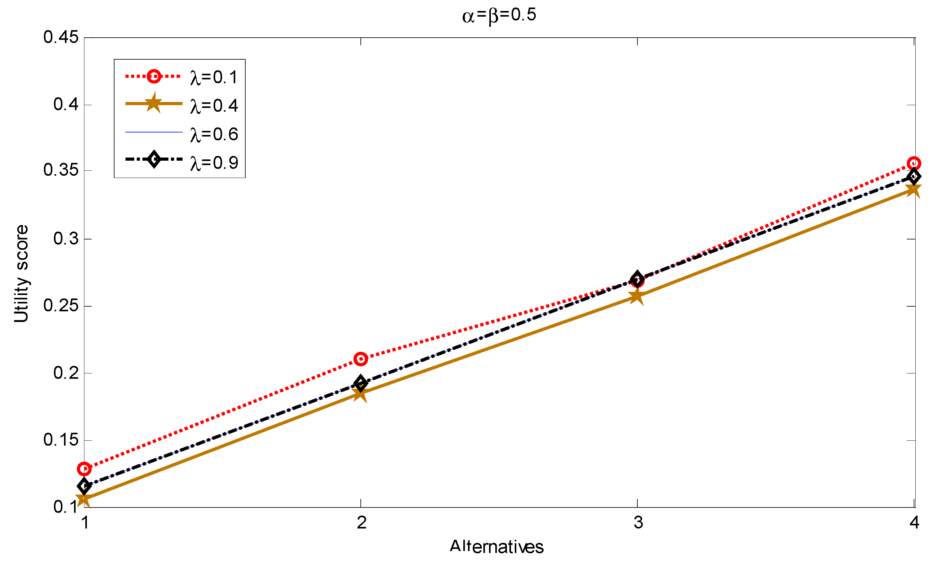
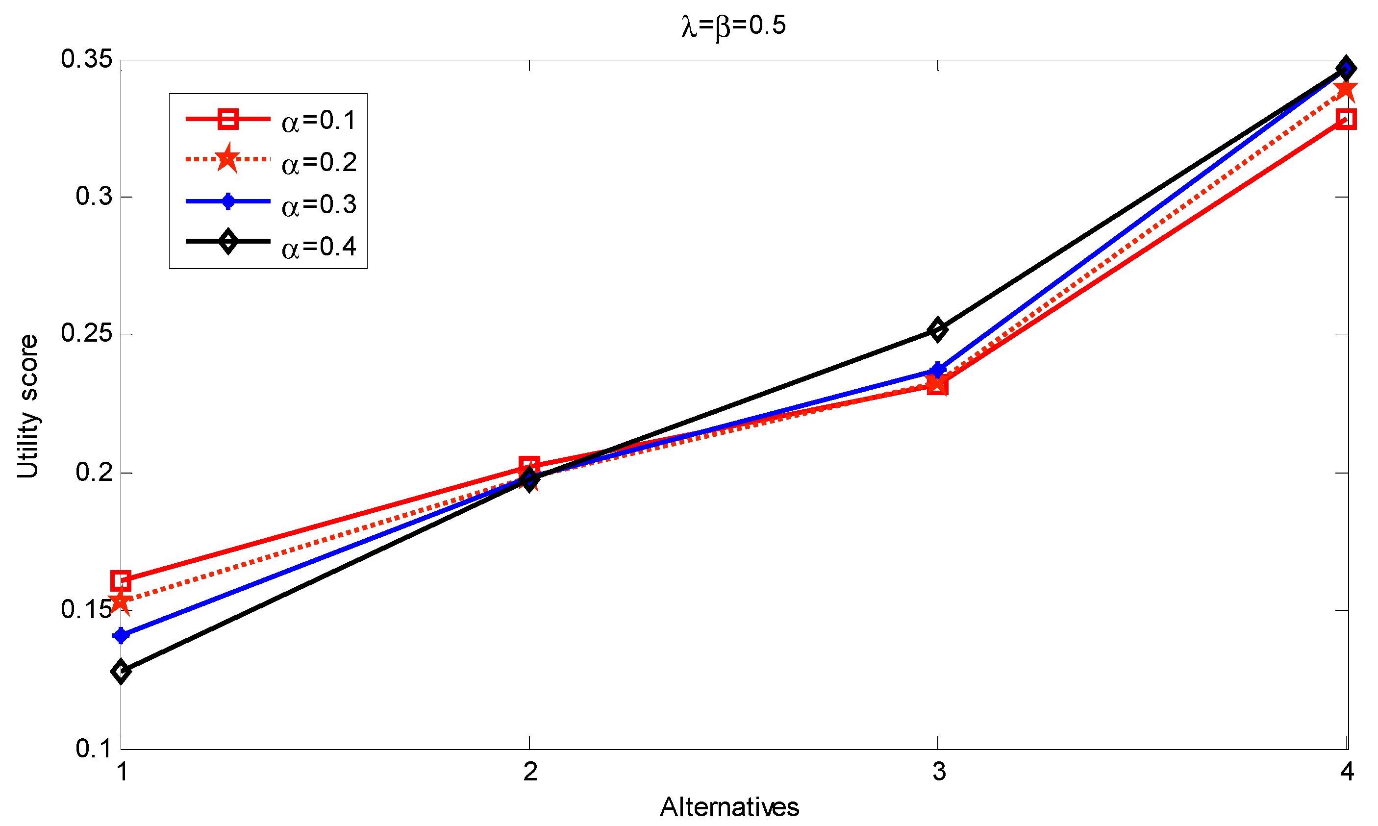
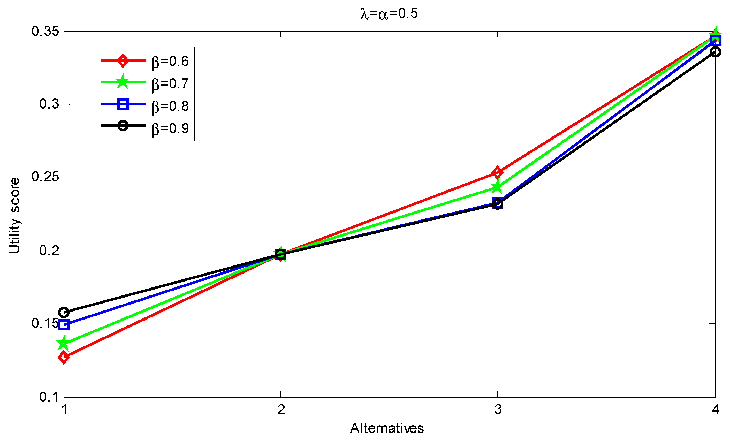
3.3. Comparative Analysis

In order to test the performance of the proposed operator, we solve the problem of the selection of the search and rescue robots by applying various aggregation operators, i.e., the weighted power average (TIFWPA) operator [31], weighted power geometric (TIFWPG) operator [36], weighted geometric mean (TIFWGM) operator [16], weighted power harmonic mean (TIFWPHM) operator [25], and weighted arithmetic mean (TIFWAM) operator [37] extended for the TIFNs. The comparative analysis is proceeded by implementing the procedure outlined in Section 3.1 and replacing the NWTIFBHM operator with the abovementioned aggregation operators. This results in the rankings of the alternatives associated with different aggregation operators. The results are summarized in Table 6.
The results in Table 6 clearly indicate that the use of the aggregation indicators which are not capable of handling extreme deviations in the data (i.e., the TIFWGM [16] and TIFWAM [37] operators) render rather different results from the rest of the operators. At the other end of the spectrum, the operators capable of accounting for possibly biased ratings (i.e., the proposed TIFWPHM operator, the weighted power average operator [31], and the weighted power geometric operator [36]) rendered similar results. It can be noted that all the operators belonging to the latter group can address the issue of the outlying data, yet the approach is different. Specifically, both the TIFWPA operator [31] and TIFWPG operator [36] allow low weights to be assigned for the outlying data and, thus, minimize their influence indirectly. On the other hand, the TIFWPHM operator [25] (here, it is the degenerate form of TrIFWPHM in [25]) focuses directly (due to its harmonic nature) on the outlying data to reduce the influence thereof on the final results of the aggregation. The NWTIFBHM showed the same best alternative, yet the ranking X3 appeared to be better in this case (the NWTIFBHM showed the same best alternative, yet the ranking X4 appeared to be better in this case).
Therefore, the proposed NWTIFBHM operator is suitable for dealing with situations where different importance of the arguments should be established given possibly biased rankings and the resulting inter-relationship patterns.
We further analyze the performance of the proposed NWTIFBHM operator by adjusting the underlying parameters. Specifically, parameters α and β determine the degree of uncertainty when constructing the ( α , β ) -cuts representing the underlying TIFNs, whereas parameter λ reflects the risk version when comparing the TIFNs. We will test the impact of changes in the values of these parameters on the results of the aggregation and ranking of the alternatives.
First, we fix the values of the parameter α = β = 0.5 and allow λ to vary, i.e., λ [ 0 , 1 ] . The ranking is repeated for several values of λ and the results are summarized in Table 7. As one can note, the resulting ranking order is stable based on NWTIFBHM with fixed (α, β). Figure 1 presents the results graphically and depicts the resulting ranking indicators for each alternative under different parameter values. As it can be seen from Figure 1, as α = β = 0.5 , given the changes of λ (within interval defined by λ [ 0 , 1 ] ), the stability of the ranking remains rather high.
Note: For the convenience of observation, the curves for λ = 0.1 and λ = 0.4 are shifted up and down by 0.01 units, respectively, and the curves for λ = 0.6 and λ = 0.9 are coincident; x-axis represents the alternatives under consideration.
Second, we allow parameters α or β to change with λ remaining fixed at 0.5 (either β or α remains fixed at 0.5 too). Since 0 α w A , 0 u A β 1 , we consider α [ 0 , 0.5 ] and β [ 0.4 , 1 ] in the numerical example. The results are given in Table 8 and Table 9. It is easy to see that the proposed approach is specific, with a rather high stability of the results.
Table 8 and Figure 2 present the results when parameter α varies for the fixed values of β and λ . As shown in Figure 2, as λ = β = 0.5 , the changes in α within α ( 0 , 0.5 ) that induce greater changes in the ranking indicator for robots X 1 , X 3 , X 4 are affected to a higher degree, but the overall stability, sorting results remain unchanged. Thus, the changes can be considered to be more quantitative than qualitative.
Table 9 and Figure 3 deal with the case where β varies for fixed α and λ . As shown in Figure 3, as λ = α = 0.5 , the values of the ranking indicator for robots S 1 , S 3 are more sensitive to changes in β , if opposed to the other alternatives. However, the overall ranking remains stable.
The analysis suggests that the proposed aggregation operator performs similarly to the other aggregation operators capable of accounting for the inter-relationships among the data. The changes in the parameters of the operator did not render significant changes in the rankings. Thus, the proposed model can be considered to be effective and stable.

4. Conclusions

Based on the Bonferroni mean, we developed the Bonferroni harmonic mean, which addresses the inter-relationships among the data to be aggregated to a higher extent. Specifically, the outlying observations receive much lower significance without any additional processing. The normalized harmonic Bonferroni mean allows for incorporating the preferences of the decision makers regarding the importance of the arguments to be aggregated. These concepts were integrated with the triangular fuzzy numbers, allowing uncertain information in the decision making problems to be represented. As a result, we have proposed the NWTIFBHM operator.
The new operator was applied in an illustrative example on a MAGDM problem. The comparative analysis comprised two directions: comparison with the existing approaches and sensitivity to changes in the underlying parameters. The analysis showed that the proposed aggregation operator is effective and is not heavily impacted by the changes in the underlying parameters.
Future research can be directed towards extension of the proposed aggregation operator by applying the generalized normalized weighted Bonferroni mean [33], probabilistic averages [38,39,40], Pythagorean fuzzy sets [12], and Choquet integrals [41], along with combinations thereof [42,43]. Simulation studies can be carried out to check the performance of the proposed approach in different settings [44] and to relate it to databases for real-life situations [45,46]. From the empirical viewpoint, applications of the NWTIFNBH operator for decisions in real-life problems can be considered across different sectors.

Author Contributions

Writing—original draft, J.Z.; Writing—review & editing, T.B. and D.S.

Funding

The work was supported in part by the National Social Science Fund Project (No. 2017YYRW07), Anhui Province Natural Science in Universities of General Project (No. TSKJ2017B22), and the general project of teaching research project of Anhui Polytechnic University (No. 2018JYXM43).

Conflicts of Interest

The authors declare no conflict of interest.

Appendix A

In this appendix, we provide the proof of Equation (16).
Proof. 
Utilizing the principles of the operational laws for the TIFNs, one can obtain
( w i ( 1 w i ) A i p ) ( w j A j q ) = ( [ w i w j ( 1 w i ) a i p a j q , w i w j ( 1 w i ) b i p b j q , w i w j ( 1 w i ) c i p c j q ] ; ω A i ω A j , u A i u A j )
Initially, one can derive that
i , j = 1 i j n ( ( w i ( 1 w i ) A i p ) ( w j A j q ) ) = ( [ i , j = 1 i j n w i w j ( 1 w i ) a i p a j q , i , j = 1 i j n w i w j ( 1 w i ) b i p b j q , i , j = 1 i j n w i w j ( 1 w i ) c i p c j q ] ; i = 1 n ω A i , i = 1 n u A i )
By exploiting the principle of mathematical induction upon n in the following manner:
(1)
when n = 2 , given (15), we can show:
i , j = 1 i j 2 ( ( w i ( 1 w i ) A i p ) ( w j A j q ) ) = ( ( w 1 ( 1 w 1 ) A 1 p ) ( w 2 A 2 q ) ) ( ( w 2 ( 1 w 2 ) A 2 p ) ( w 1 A 1 q ) ) = ( [ w 1 w 2 ( 1 w 1 ) a 1 p a 2 q + w 2 w 1 ( 1 w 2 ) a 2 p a 1 q , w 1 w 2 ( 1 w 1 ) b 1 p b 2 q + w 2 w 1 ( 1 w 2 ) b 2 p b 1 q , w 1 w 2 ( 1 w 1 ) c 1 p c 2 q + w 2 w 1 ( 1 w 2 ) c 2 p c 1 q ] ; ω A 1 ω A 2 , u A 1 u A 2 ) = ( [ i , j = 1 i j 2 w i w j ( 1 w i ) a i p a j q , i , j = 1 i j 2 w i w j ( 1 w i ) b i p b j q , i , j = 1 i j 2 w i w j ( 1 w i ) c i p c j q ] ; i = 1 2 ω A i , i = 1 2 u A i )
(2)
assume that n = k and Equation (15) holds so that
i , j = 1 i j k ( ( w i ( 1 w i ) A i p ) ( w j A j q ) ) = ( [ i , j = 1 i j k w i w j ( 1 w i ) a i p a j q , i , j = 1 i j k w i w j ( 1 w i ) b i p b j q , i , j = 1 i j k w i w j ( 1 w i ) c i p c j q ] ; i = 1 k ω A i , i = 1 k u A i )
(3)
subsequently, assume n = k + 1 and by the virtue of (15), get
i , j = 1 i j k + 1 ( ( w i ( 1 w i ) A i p ) ( w j A j q ) ) = ( i , j = 1 i j k ( ( w i ( 1 w i ) A i p ) ( w j A j q ) ) ) ( i = 1 k ( ( w i ( 1 w i ) A i p ) ( w k + 1 A k + 1 q ) ) ) ( j = 1 k ( ( w k + 1 ( 1 w k + 1 ) A k + 1 p ) ( w j A j q ) ) )
We now prove that
i = 1 k ( ( w i ( 1 w i ) A i p ) ( w k + 1 A k + 1 q ) ) = ( [ i = 1 k w i w j ( 1 w i ) a i p a j q , i = 1 k w i w j ( 1 w i ) b i p b j q , i = 1 k w i w j ( 1 w i ) c i p c j q ] ; i = 1 k ( ω A i ω A k + 1 ) , i = 1 k ( u A i u A k + 1 ) )
By applying the principle of the mathematical induction upon k .
(a)
Let k = 2 , and by the virtue of Equation (A4), one can show
i = 1 2 ( ( w i ( 1 w i ) A i p ) ( w k + 1 A k + 1 q ) ) = ( ( w 1 ( 1 w 1 ) A 1 p ) ( w k + 1 A k + 1 q ) ) ( ( w 2 ( 1 w 2 ) A 2 p ) ( w k + 1 A k + 1 q ) ) = ( [ w 1 w k + 1 ( 1 w 1 ) a 1 p a k + 1 q + w 2 w k + 1 ( 1 w 2 ) a 2 p a k + 1 q , w 1 w k + 1 ( 1 w 1 ) b 1 p b k + 1 q + w 2 w k + 1 ( 1 w 2 ) b 2 p b k + 1 q , w 1 w k + 1 ( 1 w 1 ) c 1 p c k + 1 q + w 2 w k + 1 ( 1 w 2 ) c 2 p c k + 1 q ] ; ( ω A 1 ω A k + 1 ) ( ω A 2 ω A k + 1 ) , ( u A 1 u A k + 1 ) ( u A 1 u A k + 1 ) )
= ( [ i = 1 2 w i w j ( 1 w i ) a i p a j q , i = 1 2 w i w j ( 1 w i ) b i p b j q , i = 1 2 w i w j ( 1 w i ) c i p c j q ] ; i = 1 2 ( ω A i ω A k + 1 ) , i = 1 2 ( u A i u A k + 1 ) )
(b)
Assume Equation (A4) is valid for any given k = k 0
i = 1 k 0 ( ( w i ( 1 w i ) A i p ) ( w k + 1 A k + 1 q ) ) = ( [ i = 1 k 0 w i w j ( 1 w i ) a i p a j q , i = 1 k 0 w i w j ( 1 w i ) b i p b j q , i = 1 k 0 w i w j ( 1 w i ) c i p c j q ] ; i = 1 k 0 ( ω A i ω A k + 1 ) , i = 1 k 0 ( u A i u A k + 1 ) )
(c)
Subsequently, we demonstrate that the following holds for any k = k 0 + 1 :
i = 1 k 0 + 1 ( ( w i ( 1 w i ) A i p ) ( w k + 1 A k + 1 q ) ) = i = 1 k 0 ( ( w i ( 1 w i ) A i p ) ( w k + 1 A k + 1 q ) ) ( ( w k 0 + 1 ( 1 w k 0 + 1 ) A k 0 + 1 p ) ( w k + 1 A k + 1 q ) ) = ( [ i = 1 k 0 w i w j ( 1 w i ) a i p a j q + w k 0 + 1 w k + 1 ( 1 w k 0 + 1 ) a k 0 + 1 p a k + 1 q , i = 1 k 0 w i w j ( 1 w i ) b i p b j q + w k 0 + 1 w k + 1 ( 1 w k 0 + 1 ) b k 0 + 1 p b k + 1 q , i = 1 k 0 w i w j ( 1 w i ) c i p c j q + w k 0 + 1 w k + 1 ( 1 w k 0 + 1 ) c k 0 + 1 p c k + 1 q ] ; i = 1 k 0 ( ω A i ω A k + 1 ) ( ω A k 0 + 1 ω A k + 1 ) , i = 1 k 0 ( u A i u A k + 1 ) ( u A k 0 + 1 u A k + 1 ) )
Clearly,
i = 1 k ( ω A i ω A k + 1 ) = i = 1 k + 1 ω A i , i = 1 k ( u A i u A k + 1 ) = i = 1 k + 1 u A i
Hence,
i = 1 k ( ( w i ( 1 w i ) A i p ) ( w k + 1 A k + 1 q ) ) = ( [ i = 1 k w i w k + 1 ( 1 w i ) a i p a k + 1 q , i = 1 k w i w k + 1 ( 1 w i ) b i p b k + 1 q , i = 1 k w i w k + 1 ( 1 w i ) c i p c k + 1 q ] ; i = 1 k + 1 ω A i , i = 1 k + 1 u A i )
Similarly,
j = 1 k ( ( w k + 1 ( 1 w k + 1 ) A k + 1 p ) ( w j A j q ) ) = ( [ j = 1 k w k + 1 w j ( 1 w k + 1 ) a k + 1 p a j q , j = 1 k w k + 1 w j ( 1 w k + 1 ) b k + 1 p b j q , j = 1 k w k + 1 w j ( 1 w k + 1 ) c k + 1 p c j q ] ; j = 1 k + 1 ω A j , j = 1 k + 1 u A j )
From Equations (A3), (A8) and (A9), we get
i , j = 1 i j k + 1 ( ( w i ( 1 w i ) A i p ) ( w j A j q ) ) = ( [ i , j = 1 i j k w i w j ( 1 w i ) a i p a j q , i , j = 1 i j k w i w j ( 1 w i ) b i p b j q , i , j = 1 i j k w i w j ( 1 w i ) c i p c j q ] ; i = 1 k ω A i , i = 1 k u A i ) ( [ i = 1 k w i w k + 1 ( 1 w i ) a i p a k + 1 q , i = 1 k w i w k + 1 ( 1 w i ) b i p b k + 1 q , i = 1 k w i w k + 1 ( 1 w i ) c i p c k + 1 q ] ; i = 1 k + 1 ω A i , i = 1 k + 1 u A i ) ( [ j = 1 k w k + 1 w j ( 1 w k + 1 ) a k + 1 p a j q , j = 1 k w k + 1 w j ( 1 w k + 1 ) b k + 1 p b j q , j = 1 k w k + 1 w j ( 1 w k + 1 ) c k + 1 p c j q ] ; j = 1 k + 1 ω A j , j = 1 k + 1 u A j ) = ( [ i , j = 1 i j k + 1 w i w j ( 1 w i ) a i p a j q , i , j = 1 i j k + 1 w i w j ( 1 w i ) b i p b j q , i , j = 1 i j k + 1 w i w j ( 1 w i ) c i p c j q ] ; i = 1 k + 1 ω A i , i = 1 k + 1 u A i )
As a result, Equation (A1) is valid for n = k + 1 . Therefore, Equation (A1) is valid for any n . Considering Equation (A1) alongside operational law (3)
1 ( i , j = 1 i j k + 1 ( ( w i ( 1 w i ) A i p ) ( w j A j q ) ) ) 1 p + q = ( [ 1 ( i , j = 1 i j k + 1 w i w j ( 1 w i ) a i p a j q ) 1 p + q , 1 ( i , j = 1 i j k + 1 w i w j ( 1 w i ) b i p b j q ) 1 p + q , 1 ( i , j = 1 i j k + 1 w i w j ( 1 w i ) c i p c j q ) 1 p + q ] ; i = 1 k + 1 ω A i , i = 1 k + 1 u A i )
Exploiting Equation (A10) as well as operational law (4), one can show that
N W T I F B H M p , q ( A 1 , A 2 , , A n ) = ( [ 1 ( i , j = 1 i j n w i w j ( 1 w i ) a i p a j q ) 1 p + q , 1 ( i , j = 1 i j n w i w j ( 1 w i ) b i p b j q ) 1 p + q , 1 ( i , j = 1 i j n w i w j ( 1 w i ) c i p c j q ) 1 p + q ] ; i = 1 n ω A i , i = 1 n u A i )
As long as a i b i c i , for all i = 1 , 2 , , n . By the virtue of the property associated with the NWBHM, one can show that
1 ( i , j = 1 i j n w i w j ( 1 w i ) a i p a j q ) 1 p + q 1 ( i , j = 1 i j n w i w j ( 1 w i ) b i p b j q ) 1 p + q 1 ( i , j = 1 i j n w i w j ( 1 w i ) c i p c j q ) 1 p + q
Also,
0 i = 1 n ω A i + i = 1 n u A i 1
From Equations (A12) and (A13), N W T I F B H M p , q is a TIFN.

References

  1. Atanassov, K.T. Intuitionistic fuzzy sets. Fuzzy Sets Syst. 1986, 20, 87–96. [Google Scholar] [CrossRef]
  2. Atanassov, K.T. More on intuitionistic fuzzy sets. Fuzzy Sets Syst. 1989, 51, 117–118. [Google Scholar] [CrossRef]
  3. Liu, P.D.; Chen, S.M. Group Decision Making Based on Heronian Aggregation Operators of Intuitionistic Fuzzy Numbers. IEEE Trans. Cybern. 2017, 47, 2514–2530. [Google Scholar] [CrossRef] [PubMed]
  4. Xu, Z.S.; Yager, R.R. Some geometric aggregation operators based on intuitionistic fuzzy sets. Int. J. Gen. Syst. 2006, 35, 417–433. [Google Scholar] [CrossRef]
  5. Peng, B.; Zhou, J.M.; Peng, D.H. Cloud model based approach to group decision making under uncertain pure linguistic information. J. Intell. Fuzzy Syst. 2017, 32, 1959–1968. [Google Scholar] [CrossRef]
  6. Atanassov, K.T.; Pasi, G.; Yager, R.R. Intuitionistic fuzzy interpretations of multi-criteria multi-person and multi-measurement tool decision making. Int. J. Gen. Syst. 2005, 36, 859–868. [Google Scholar] [CrossRef]
  7. Liang, C.; Zhao, S.; Zhang, J. Multi-criteria group decision making method based on generalized intuitionistic trapezoidal fuzzy prioritized aggregation operators. Int. J. Mach. Learn. Cybern. 2017, 8, 597–610. [Google Scholar] [CrossRef]
  8. Zhao, H.; Xu, Z.S.; Ni, M.F.; Liu, S.H. Generalized Aggregation Operators for Intuitionistic Fuzzy Sets. Int. J. Intell. Syst. 2009, 25, 1–30. [Google Scholar] [CrossRef]
  9. Chu, Y.C.; Liu, P.D. Some two-dimensional uncertain linguistic Heronian mean operators and their application in multiple-attribute decision making. Neural Comput. Appl. 2015, 26, 1461–1480. [Google Scholar] [CrossRef]
  10. Li, D.F. A ratio ranking method of triangular intuitionistic fuzzy numbers and its application to MADM problems. Comput. Math. Appl. 2010, 60, 1557–1570. [Google Scholar] [CrossRef]
  11. Su Mail, W.; Zhou, J.; Zeng, S.; Zhang, C.; Yu, K. A Novel Method for Intuitionistic Fuzzy MAGDM with Bonferroni Weighted Harmonic Means. Recent Patents Comput. Sci. 2017, 10, 178–189. [Google Scholar]
  12. Zeng, S.Z.; Xiao, Y. A method based on TOPSIS and distance measures for hesitant fuzzy multiple attribute decision making. Technol. Econ. Dev. Econ. 2018, 24, 969–983. [Google Scholar] [CrossRef]
  13. Wang, J.Q. Overview on fuzzy multi-criteria decision-making approach. Control Decis. 2008, 23, 601–607. [Google Scholar]
  14. Fan, C.X.; Ye, J.; Hu, K.L.; Fan, E. Bonferroni Mean Operators of Linguistic Neutrosophic Numbers and Their Multiple Attribute Group Decision-Making Methods. Information 2017, 8, 107. [Google Scholar] [CrossRef]
  15. Wang, J.P.; Dong, J.Y. Method of intuitionistic trapezoidal fuzzy number for multi-attribute group decision. Control Decis. 2010, 25, 773–776. [Google Scholar]
  16. Wu, J.; Cao, Q.W. Same families of geometric aggregation operators with intuitionistic trapezoidal fuzzy numbers. Appl. Math. Model. 2013, 37, 318–327. [Google Scholar] [CrossRef]
  17. Bonferroni, C. Sulle medie multiple di potenze. Boll. Matemat. Ital. 1950, 5, 267–270. [Google Scholar]
  18. Yager, R.R. On generalized Bonferroni mean operators for multicriteria aggregation. Int. J. Approx. Reason. 2009, 50, 1279–1286. [Google Scholar] [CrossRef]
  19. Choquet, G. Theory of capacities. Ann. Inst. Fourier 1955, 50, 131–295. [Google Scholar] [CrossRef]
  20. Beliakov, G.; James, S.; Mordelová, J.; Rückschlossová, T.; Yager, R.R. Generalized Bonferroni mean operators in multi-criteria aggregation. Fuzzy Sets Syst. 2010, 161, 2227–2242. [Google Scholar] [CrossRef]
  21. Xu, Z.S.; Yager, R.R. Intuitionistic Fuzzy Bonferroni Means. IEEE Trans. Syst. Man Cybern. Part B Cybern. 2011, 41, 568–578. [Google Scholar]
  22. Dutta, B.; Guha, D. Trapezoidal Intuitionistic Fuzzy Bonferroni Means and Its Application in Multi-attribute Decision Making. In Proceedings of the 2013 IEEE International Conference on Fuzzy Systems (FUZZ), Hyderabad, India, 7–10 July 2013. [Google Scholar]
  23. Xu, Z.S. Uncertain Bonferroni Mean operators. Int. J. Comput. Intell. Syst. 2010, 3, 761–769. [Google Scholar] [CrossRef]
  24. Xia, M.; Xu, Z.S.; Zhu, B. Generalized Intuitionistic Fuzzy Bonferroni Means. Int. J. Intell. Syst. 2012, 27, 23–47. [Google Scholar] [CrossRef]
  25. Das, S.; Guha, D. Power harmonic aggregation operator with Trapezoidal intuitionistic fuzzy numbers for solving MAGDM problems. Iranian J. Fuzzy Syst. 2015, 12, 41–74. [Google Scholar]
  26. Xu, Z.S. Fuzzy harmonic mean operators. Int. J. Intell. Syst. 2009, 24, 152–172. [Google Scholar] [CrossRef]
  27. Wei, G.W. FIOWHM operator and its application to multiple attribute group decision making. Expert Syst. Appl. 2011, 38, 2984–2989. [Google Scholar] [CrossRef]
  28. Sun, H.; Sun, M. Generalized Bonferroni harmonic mean operators and their application to multiple attribute decision making. J. Comput. Inf. Syst. 2012, 8, 5717–5724. [Google Scholar]
  29. Park, J.H.; Park, E.J. Generalized Fuzzy Bonferroni Harmonic Mean Operators and Their Applications in Group Decision Making. J. Appl. Math. 2013, 2013, 1–14. [Google Scholar] [CrossRef]
  30. Liu, P.D.; Li, H.G. Interval-Valued Intuitionistic Fuzzy Power Bonferroni Aggregation Operators and Their Application to Group Decision Making. Cogn. Comput. 2017, 9, 1–19. [Google Scholar] [CrossRef]
  31. Wan, S.P. Power average operators of trapezoidal intuitionistic fuzzy numbers and application to multi-attribute group decision making. Appl. Math. Model. 2013, 37, 4112–4126. [Google Scholar] [CrossRef]
  32. Li, D.F. Decision and Game Theory in Management with Intuitionistic Fuzzy Sets; Springer: Berlin/Heidelberg, Germany, 2014. [Google Scholar]
  33. Zhou, W.; He, J.M. Intuitionistic Fuzzy Normalized Weighted Bonferroni Mean and Its Application in Multicriteria Decision Making. J. Appl. Math. 2012, 2012, 1–22. [Google Scholar] [CrossRef]
  34. Xu, Z.S.; Da, Q.L. A likelihood based method for priorities of interval judgment matrices. Chin. J. Manag. Sci. 2003, 11, 63–65. [Google Scholar]
  35. Micire, M.J. Evolution and field performance of a rescue robot. J. Field Robot. 2008, 25, 17–30. [Google Scholar] [CrossRef]
  36. Wan, S.P.; Dong, J.Y. Power geometric operators of trapezoidal intuitionistic fuzzy numbers and application to multi-attribute group decision making. Appl. Soft Comput. 2015, 29, 153–168. [Google Scholar] [CrossRef]
  37. Wei, G.W. Some arithmetic aggregation operators with intuitionistic trapezoidal fuzzy numbers and their application to group decision making. J. Comput. 2010, 5, 345–351. [Google Scholar] [CrossRef]
  38. Merigó, J.M.; Wei, G.W. Probabilistic aggregation operators and their application in uncertain multi-person decision making. Technol. Econ. Dev. 2011, 17, 335–351. [Google Scholar] [CrossRef]
  39. Merigó, J.M. The probabilistic weighted average and its application in multi-person decision making. Int. J. Intell. Syst. 2012, 27, 457–476. [Google Scholar] [CrossRef]
  40. Xu, Z.S.; Da, Q.L. An overview of operators for aggregating information. Int. J. Intell. Syst. 2003, 18, 953–968. [Google Scholar] [CrossRef]
  41. Bolton, J.; Gader, P.; Wilson, J.N. Discrete Choquet integral as a distance metric. IEEE Trans. Fuzzy Syst. 2008, 16, 1107–1110. [Google Scholar] [CrossRef]
  42. Xu, Z.S.; Da, Q.L. The Uncertain OWA operator. Int. J. Intell. Syst. 2002, 17, 569–575. [Google Scholar] [CrossRef]
  43. Zeng, S.Z.; Su, W.H.; Zhang, C.H. A Novel Method Based on Induced Aggregation Operator for Classroom Teaching Quality Evaluation with Probabilistic and Pythagorean Fuzzy Information. Eurasia J. Math. Sci. Technol. Educ. 2018, 14, 3205–3212. [Google Scholar] [CrossRef]
  44. Mukhametzyanov, I.; Pamucar, D. A sensitivity analysis in MCDM problems: A statistical approach. Decis. Mak. Appl. Manag. Eng. 2018, 1, 51–80. [Google Scholar] [CrossRef]
  45. Yi, P.; Li, W.; Li, L. Evaluation and Prediction of City Sustainability Using MCDM and Stochastic Simulation Methods. Sustainability 2018, 10, 3771. [Google Scholar] [CrossRef]
  46. Zhu, B.; Xu, Z. Probability-hesitant fuzzy sets and the representation of preference relations. Technol. Econ. Dev. Econ. 2018, 24, 1029–1040. [Google Scholar] [CrossRef]
Figure 1. Sensitivity analysis of NWTIFBHM evaluation results ( α = β = 0.5 ).
Symmetry 11 00218 g001
Figure 2. Sensitivity analysis of NWTIFBHM evaluation results ( λ = β = 0.5 ).
Symmetry 11 00218 g002
Figure 3. Sensitivity analysis of NWTIFBHM evaluation results ( λ = α = 0.5 ).
Symmetry 11 00218 g003
Table 1. Decision matrix A 1 given by expert D 1 .
AlternativeC1C2C3C4
X1([0.05,0.1,0.15];0.7,0.2)([0.1,0.15,0.2];0.5,0.4)([0.1,0.2,0.25];0.6,0.4)([0.75,0.8,0.9];0.8,0.1)
X2([0.2,0.25,0.3];0.6,0.3)([0.8,0.85,0.95];0.8,0.2)([0.15,0.2,0.25];0.7,0.2)([0.2,0.25,0.3];0.6,0.3)
X3([0.1,0.2,0.3];0.5,0.4)([0.1,0.2,0.3];0.7,0.2)([0.85,0.9,0.95];0.6,0.3)([0.15,0.2,0.3];0.7,0.1)
X4([0.85,0.9,0.95];0.5,0.3)([0.2,0.3,0.35];0.6,0.3)([0.15,0.3,0.4];0.5,0.2)([0.1,0.25,0.35];0.8,0.1)
Table 2. Decision matrix A 2 given by expert D 2 .
AlternativeC1C2C3C4
X1([0.05,0.15,0.25];0.6,0.4)([0.1,0.15,0.2];0.6,0.3)([0.1,0.15,0.2];0.6,0.4)([0.85,0.9,0.95];0.6,0.3)
X2([0.15,0.25,0.3];0.6,0.3)([0.75,0.85,0.95];0.7,0.2)([0.15,0.2,0.25];0.7,0.2)([0.2,0.25,0.3];0.6,0.4)
X3([0.75,0.8,0.85];0.9,0.1)([0.1,0.2,0.25];0.5,0.3)([0.1,0.25,0.3];0.7,0.2)([0.15,0.25,0.3];0.8,0.1)
X4([0.1,0.3,0.4];0.6,0.2)([0.2,0.25,0.3];0.8,0.1)([0.8,0.85,0.95];0.7,0.3)([0.1,0.25,0.35];0.5,0.4)
Table 3. Decision matrix A 3 given by expert D 3 .
AlternativeC1C2C3C4
X1([0.8,0.85,0.9];0.9,0.1)([0.2,0.25,0.3];0.5,0.4)([0.1,0.2,0.25];0.6,0.4)([0.15,0.2,0.3];0.8,0.1)
X2([0.15,0.25,0.3];0.6,0.2)([0.1,0.15,0.2];0.6,0.2)([0.15,0.2,0.25];0.7,0.2)([0.8,0.85,0.95];0.8,0.2)
X3([0.2,0.25,0.3];0.5,0.4)([0.05,0.1,0.15];0.7,0.2)([0.85,0.9,0.95];0.6,0.25)([0.15,0.2,0.25];0.7,0.1)
X4([0.1,0.2,0.25];0.7,0.2)([0.75,0.8,0.9];0.6,0.2)([0.2,0.25,0.3];0.5,0.4)([0.1,0.25,0.3];0.6,0.3)
Table 4. Decision matrix A 4 given by expert D 4 .
AlternativeC1C2C3C4
X1([0.15,0.2,0.3];0.5,0.5)([0.25,0.3,0.35];0.4,0.4)([0.75,0.85,0.9];0.5,0.4)([0.2,0.35,0.4];0.7,0.2)
X2([0.85,0.9,0.95];0.8,0.1)([0.05,0.1,0.15];0.6,0.3)([0.2,0.25,0.3];0.7,0.2)([0.1,0.15,0.2];0.9,0.1)
X3([0.2,0.25,0.3];0.5,0.4)([0.8,0.85,0.9];0.8,0.1)([0.05,0.1,0.15];0.7,0.2)([0.25,0.3,0.35];0.5,0.4)
X4([0.1,0.2,0.3];0.7,0.2)([0.15,0.25,0.35];0.5,0.3)([0.25,0.3,0.35];0.6,0.3)([0.8,0.9,0.95];0.6,0.2)
Table 5. The overall performance value A t i , ( i , t = 1 , 2 , 3 , 4 ) by decision makers.
AlternativeD1D2D3D4
X1([0.1196,0.2204,0.2640];
0.5,0.4)
([0.1196,0.2304,0.2827];
0.6,0.4)
([0.3140,0.4742,0.5667];
0.5,0.4)
([0.4376,0.5420,0.6837];
0.5,0.4)
X2([0.3673,0.4620,0.5584];
0.6,0.3)
([0.3225,0.4620,0.5584];
0.6,0.4)
([0.2017,0.2990,0.3778];
0.6,0.2)
([0.2333,0.3562,0.4641];
0.6,0.3)
X3([0.2598,0.4703,0.6546];
0.5,0.4)
([0.2328,0.4727,0.5643];
0.5,0.3)
([0.2533,0.3826,0.4945];
0.5,0.4)
([0.2190,0.3363,0.4401];
0.5,0.4)
X4([0.3815,0.6127,0.7405];
0.5,0.3)
([0.3420,0.5948,0.7293];
0.5,0.4)
([0.3058,0.4600,0.5559];
0.5,0.4)
([0.2360,0.3796,0.5107];
0.5,0.3)
Table 6. The ranking order rendered by the different methods.
MethodRanking OrderBest Alternative
TIFWPA X 4 X 2 X 1   X 3 X 4
TIFWPG X 4 X 2 X 1   X 3 X 4
TIFWGM X 1 X 4 X 2     X 3 X 1
TIFWAM X 3 X 4 X 1     X 2 X 3
TIFWPHM X 4 X 2 X 1   X 3 X 4
NWTIFBHM X 4 X 3 X 2     X 1 X 4
Table 7. The ordering of different λ based on NWTIFBHM operator ( α = β = 0.5 ).
λ Ranking IndexRanking Order
λ = 0.1 R I ( A 1 ) = 0.1178 , R I ( A 2 ) = 0.2004 , R I ( A 3 ) = 0.2588 , R I ( A 4 ) = 0.3462 X 4 X 3 X 2     X 1
λ = 0.4 R I ( A 1 ) = 0.1154 , R I ( A 2 ) = 0.1945 , R I ( A 3 ) = 0.2671 , R I ( A 4 ) = 0.3462 X 4 X 3 X 2     X 1
λ = 0.6 R I ( A 1 ) = 0.1154 , R I ( A 2 ) = 0.1923 , R I ( A 3 ) = 0.2692 , R I ( A 4 ) = 0.3462 X 4 X 3 X 2     X 1
λ = 0.9 R I ( A 1 ) = 0.1154 , R I ( A 2 ) = 0.1923 , R I ( A 3 ) = 0.2692 , R I ( A 4 ) = 0.3462 X 4 X 3 X 2     X 1
Table 8. The ordering of different α based on NWTIFBHM operator ( λ = β = 0.5 ).
α Ranking IndexRanking Order
α = 0.1 R I ( A 1 ) = 0.1608 , R I ( A 2 ) = 0.2020 , R I ( A 3 ) = 0.2317 , R I ( A 4 ) = 0.3285 X 4 X 3 X 2     X 1
α = 0.2 R I ( A 1 ) = 0.1535 , R I ( A 2 ) = 0.1984 , R I ( A 3 ) = 0.2325 , R I ( A 4 ) = 0.3387 X 4 X 3 X 2     X 1
α = 0.3 R I ( A 1 ) = 0.1412 , R I ( A 2 ) = 0.1983 , R I ( A 3 ) = 0.2374 , R I ( A 4 ) = 0.3462 X 4 X 3 X 2     X 1
α = 0.4 R I ( A 1 ) = 0.1276 , R I ( A 2 ) = 0.1978 , R I ( A 3 ) = 0.2516 , R I ( A 4 ) = 0.3462 X 4 X 3 X 2     X 1
Table 9. The ordering of different β based on NWTIFBHM operator ( λ = α = 0.5 ).
β Ranking IndexRanking Order
β = 0.6 R I ( A 1 ) = 0.1269 , R I ( A 2 ) = 0.1971 , R I ( A 3 ) = 0.2530 , R I ( A 4 ) = 0.3462 X 4 X 3 X 2     X 1
β = 0.7 R I ( A 1 ) = 0.1363 , R I ( A 2 ) = 0.1974 , R I ( A 3 ) = 0.2432 , R I ( A 4 ) = 0.3462 X 4 X 3 X 2     X 1
β = 0.8 R I ( A 1 ) = 0.1494 , R I ( A 2 ) = 0.1975 , R I ( A 3 ) = 0.2326 , R I ( A 4 ) = 0.3435 X 4 X 3 X 2     X 1
β = 0.9 R I ( A 1 ) = 0.1574 , R I ( A 2 ) = 0.1976 , R I ( A 3 ) = 0.2320 , R I ( A 4 ) = 0.3361 X 4 X 3 X 2     X 1

