MHD Flow and Heat Transfer in Sodium Alginate Fluid with Thermal Radiation and Porosity Effects: Fractional Model of Atangana–Baleanu Derivative of Non-Local and Non-Singular Kernel

 , ,
, , 

Abstract
1. Introduction
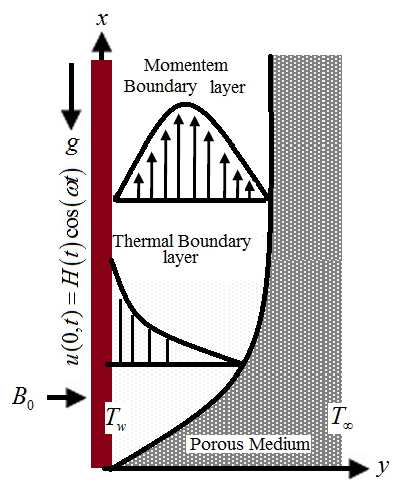
2. Mathematical Framing of the Problem
3. Problem Solution, Skin Friction, and Nusselt Number
4. Skin Friction and Nusselt Number
5. Discussion
6. Conclusions
- ➣
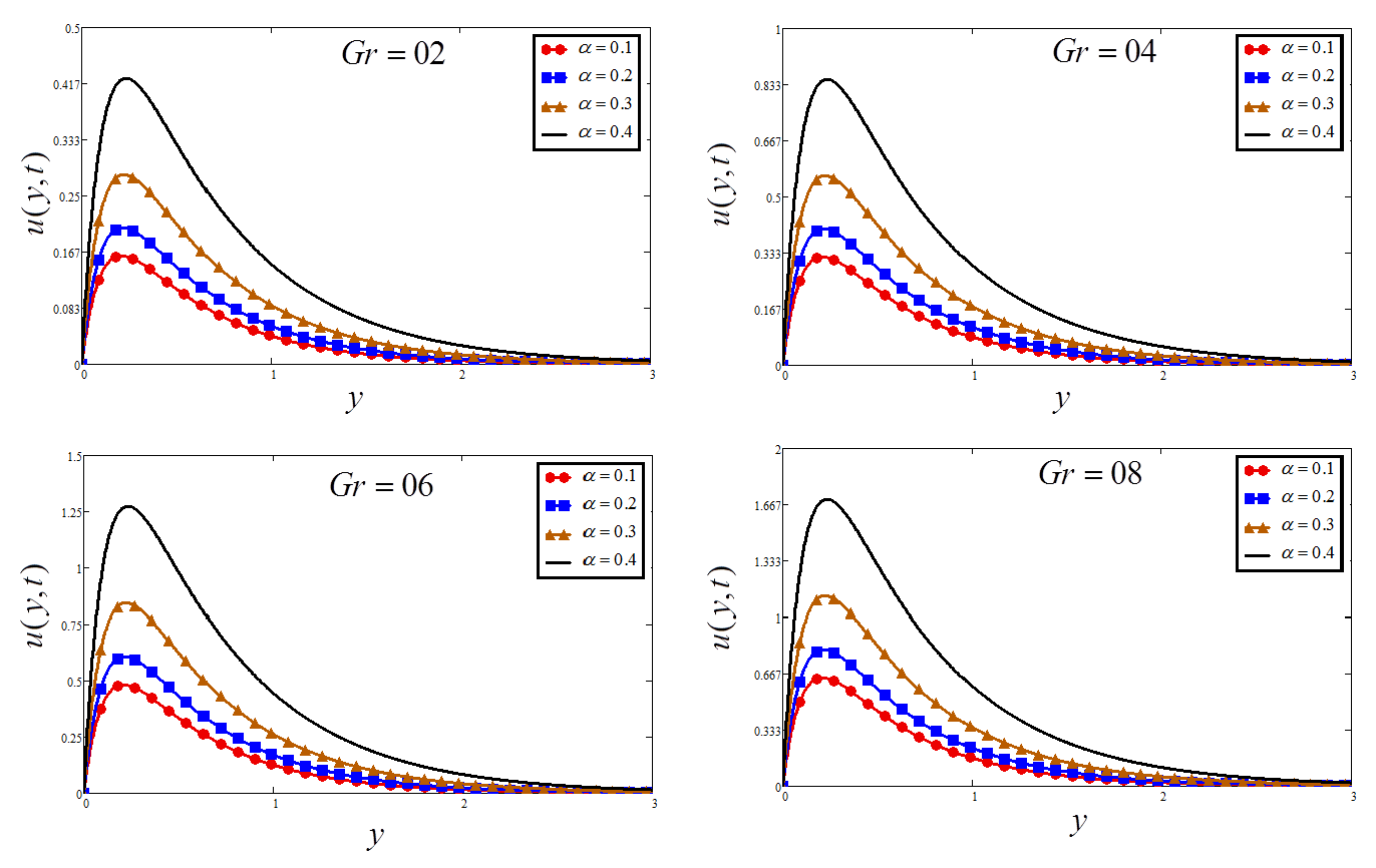
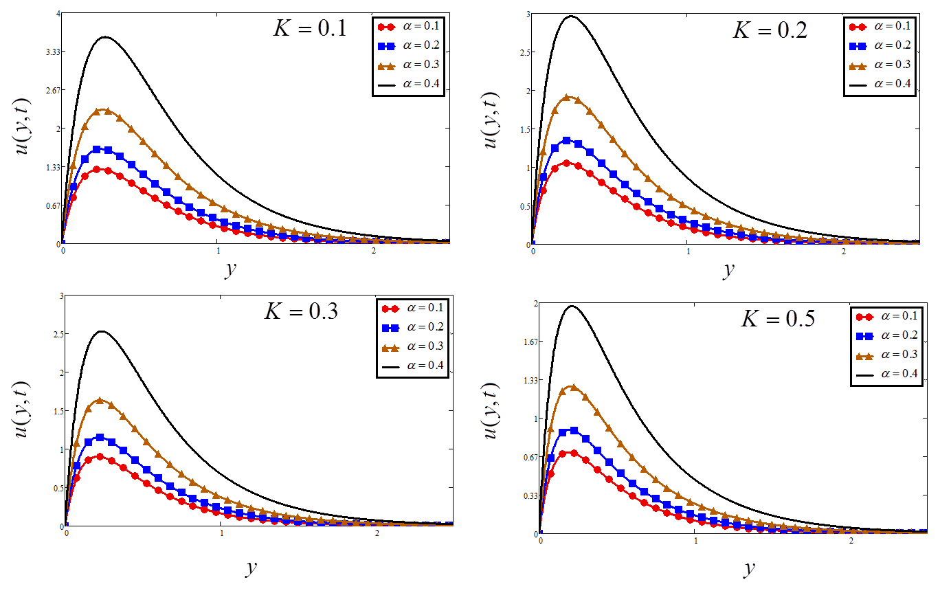
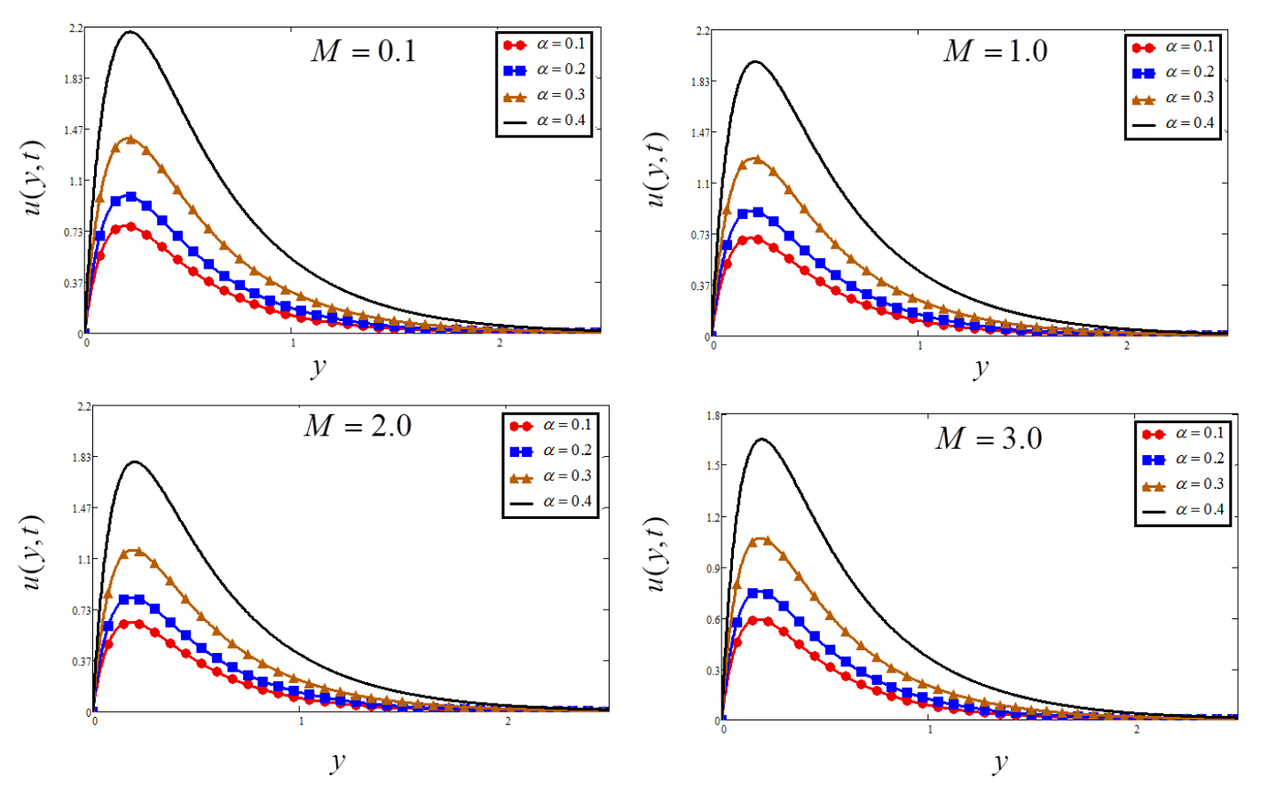
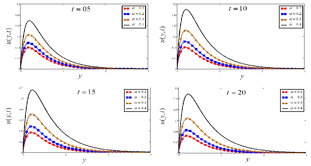
- Velocity rises for a large value of , and
- ➣
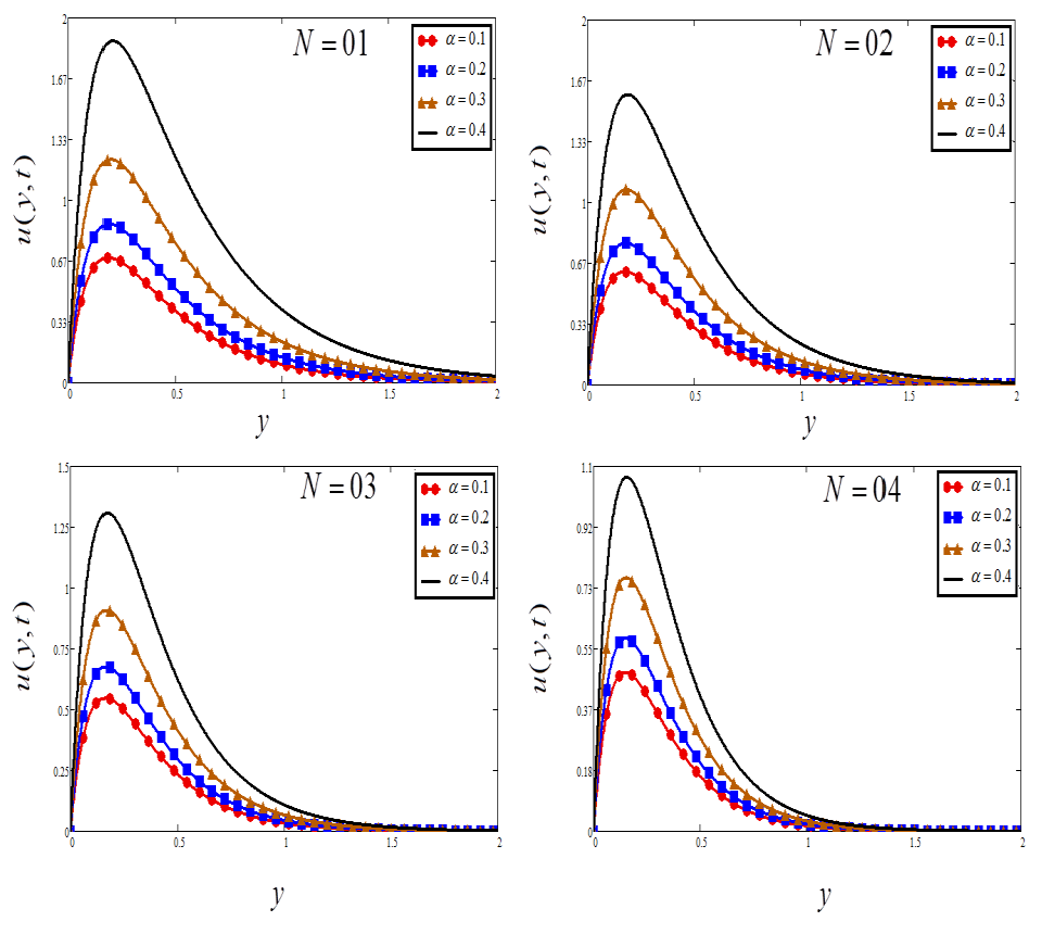
- Velocity reduces for a large value of , and .
- ➣
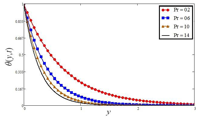
- Temperature is increased by increasing and , while decreasing with the increase of .
- ➣
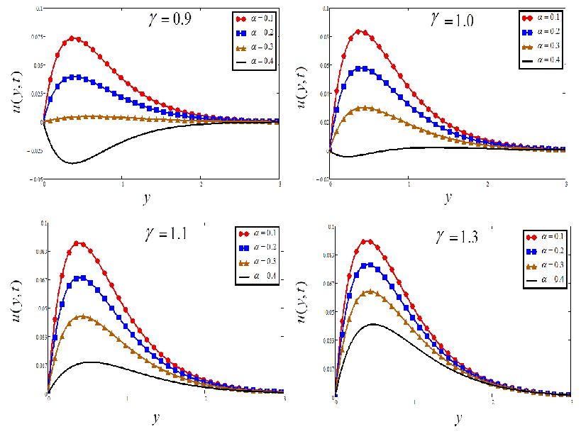
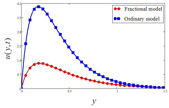
- The temperature and velocity of the fractional fluid model converge faster compared to an ordinary fluid model.
- ➣
- The Atangana–Baleanu fractional model reduced the velocity profile up to 45.76% and temperature profile up to 13.74% compared to an ordinary model.
- ➣
- The researchers extend this work for different kind of nanofluids.
- ➣
- The authors also can take this model in different geometries.
Author Contributions
Funding
Conflicts of Interest
References
- Casson, N. A flow equation for the pigment oil suspensions of the printing ink type. In Rheology of Disperse Systems; Pergamon Press: New York, NY, USA, 1959; Volume 84, p. e102. [Google Scholar]
- Qasim, M.; Ahmad, B. Numerical solution for the Blasius flow in Casson fluid with viscous dissipation and convective boundary conditions. Heat Transf. Res. 2015, 46, 689–697. [Google Scholar] [CrossRef]
- Shehzad, S.A.; Hayat, T.; Qasim, M.; Asghar, S. Effects of mass transfer on MHD flow of Casson fluid with chemical reaction and suction. Braz. J. Chem. Eng. 2013, 30, 187–195. [Google Scholar] [CrossRef]
- Qasim, M.; Noreen, S. Heat transfer in the boundary layer flow of a Casson fluid over a permeable shrinking sheet with viscous dissipation. Eur. Phys. J. Plus 2014, 129, 7. [Google Scholar] [CrossRef]
- Mukhopadhyay, S.; Mandal, I.C. Boundary layer flow and heat transfer of a Casson fluid past a symmetric porous wedge with surface heat flux. Chin. Phys. B 2014, 23, 044702. [Google Scholar] [CrossRef]
- Siddiqui, A.M.; Farooq, A.A.; Rana, M.A. A mathematical model for the flow of a Casson fluid due to metachronal beating of cilia in a tube. Sci. World J. 2015, 2015, 487819. [Google Scholar] [CrossRef] [PubMed]
- Hayat, T.; Shehzad, S.A.; Alsaedi, A.; Alhothuali, M.S. Mixed convection stagnation point flow of Casson fluid with convective boundary conditions. Chin. Phys. Lett. 2012, 29, 114704. [Google Scholar] [CrossRef]
- Asjad, M.I.; Miraj, F.; Khan, I. Soret effects on simultaneous heat and mass transfer in MHD viscous fluid through a porous medium with uniform heat flux and Atangana-Baleanu fractional derivative approach. Eur. Phys. J. Plus 2018, 133, 224. [Google Scholar] [CrossRef]
- Atangana, A.; Baleanu, D. Caputo-Fabrizio derivative applied to groundwater flow within confined aquifer. J. Eng. Mech. 2017, 143, D4016005. [Google Scholar] [CrossRef]
- Atangana, A.; Goufo, E.F.D. The Caputo-Fabrizio fractional derivative applied to a singular perturbation problem. Int. J. Math. Model. Numer. Optim. 2019, 9, 241–253. [Google Scholar]
- Aliyu, A.I.; Inc, M.; Yusuf, A.; Baleanu, D. A fractional model of vertical transmission and cure of vector-borne diseases pertaining to the Atangana–Baleanu fractional derivatives. Chaos Solitons Fractals 2018, 116, 268–277. [Google Scholar] [CrossRef]
- Koca, I. Modelling the spread of Ebola virus with Atangana-Baleanu fractional operators. Eur. Phys. J. Plus 2018, 133, 100. [Google Scholar] [CrossRef]
- Azhar, W.A.; Vieru, D.; Fetecau, C. Free convection flow of some fractional nanofluids over a moving vertical plate with uniform heat flux and heat source. Phys. Fluids 2017, 29, 082001. [Google Scholar] [CrossRef]
- Fetecau, C.; Vieru, D.; Azhar, W. Natural convection flow of fractional nanofluids over an isothermal vertical plate with thermal radiation. Appl. Sci. 2017, 7, 247. [Google Scholar] [CrossRef]
- Sheikh, N.A.; Ali, F.; Khan, I.; Gohar, M.; Saqib, M. On the applications of nanofluids to enhance the performance of solar collectors: A comparative analysis of Atangana–Baleanu and Caputo–Fabrizio fractional models. Eur. Phy. J. Plus 2017, 132, 540. [Google Scholar] [CrossRef]
- Karaagac, B. Two step Adams Bashforth method for time fractional Tricomi equation with non-local and non-singular Kernel. Chaos Solitons Fractals 2019, 128, 234–241. [Google Scholar] [CrossRef]
- Ali, F.; Saqib, M.; Khan, I.; Sheikh, N.A. Application of Caputo-Fabrizio derivatives to MHD free convection flow of generalized Walters’-B fluid model. Eur. Phys. J. Plus 2016, 131, 377. [Google Scholar] [CrossRef]
- Saqib, M.; Khan, I.; Shafie, S. Application of Atangana–Baleanu fractional derivative to MHD channel flow of CMC-based-CNT’s nanofluid through a porous medium. Chaos Solitons Fractals 2018, 116, 79–85. [Google Scholar] [CrossRef]
- Abro, K.A.; Khan, I.; Tassaddiq, A. Application of Atangana-Baleanu fractional derivative to convection flow of MHD Maxwell fluid in a porous medium over a vertical plate. Math. Model. Nat. Phenom. 2018, 13, 1. [Google Scholar] [CrossRef]
- Abro, K.A.; Khan, I.; Nisar, K.S.; Alsagri, A.S. Efects of carbon nanotubes on Magnetohydrodynamic flow of methanol based nanofluids via Atangana-Baleanu and Caputo-fabrizio fractional derivatives. Therm. Sci. 2019, 23, 883–898. [Google Scholar]
- Yavuz, M.; Özdemir, N. Comparing the new fractional derivative operators involving exponential and Mittag-Leffler kernel. Discret. Contin. Dyn. Syst. S 2019, 13, 995–1006. [Google Scholar] [CrossRef]
- Imran, M.A.; Aleem, M.; Riaz, M.B.; Ali, R.; Khan, I. A comprehensive report on convective flow of fractional (ABC) and (CF) MHD viscous fluid subject to generalized boundary conditions. Chaos Solitons Fractals 2019, 118, 274–289. [Google Scholar] [CrossRef]
- Abro, K.A.; Khan, I. MHD flow of fractional Newtonian fluid embedded in a porous medium via Atangana-Baleanu fractional derivatives. Discret. Contin. Dyn. Syst. S 2019. [Google Scholar] [CrossRef]
- Wenchang, T.; Mingyu, X. Unsteady flows of a generalized second grade fluid with the fractional derivative model between two parallel plates. Acta Mech. 2004, 20, 471–476. [Google Scholar] [CrossRef]
- Xu, M.; Tan, W. Theoretical analysis of the velocity field, stress field and vortex sheet of generalized second order fluid with fractional anomalous diffusion. Sci. China Ser. A Math. 2001, 44, 1387–1399. [Google Scholar] [CrossRef]
- Shen, F.; Tan, W.; Zhao, Y.; Masuoka, T. The Rayleigh–Stokes problem for a heated generalized second grade fluid with fractional derivative model. Nonlinear Anal. Real World Appl. 2006, 7, 1072–1080. [Google Scholar] [CrossRef]
- Mahmood, A.; Parveen, S.; Ara, A.; Khan, N.A. Exact analytic solutions for the unsteady flow of a non-Newtonian fluid between two cylinders with fractional derivative model. Commun. Nonlinear Sci. Numer. Simul. 2009, 14, 3309–3319. [Google Scholar] [CrossRef]
- Shen, M.; Chen, S.; Liu, F. Unsteady MHD flow and heat transfer of fractional Maxwell viscoelastic nanofluid with Cattaneo heat flux and different particle shapes. Chin. J. Phys. 2018, 56, 1199–1211. [Google Scholar] [CrossRef]
- Zhang, Y.; Zhao, H.; Liu, F.; Bai, Y. Analytical and numerical solutions of the unsteady 2D flow of MHD fractional Maxwell fluid induced by variable pressure gradient. Comput. Math. Appl. 2018, 75, 965–980. [Google Scholar] [CrossRef]
- Aman, S.; Al-Mdallal, Q.; Khan, I. Heat transfer and second order slip effect on MHD flow of fractional Maxwell fluid in a porous medium. J. King Saud Univ. Sci. 2018. [Google Scholar] [CrossRef]
- Jan, S.A.A.; Ali, F.; Sheikh, N.A.; Khan, I.; Saqib, M.; Gohar, M. Engine oil based generalized brinkman-type nano-liquid with molybdenum disulphide nanoparticles of spherical shape: Atangana-Baleanu fractional model. Numer. Methods Part. Differ. Equ. 2018, 34, 1472–1488. [Google Scholar] [CrossRef]
- Owolabi, K.M.; Atangana, A. On the formulation of Adams-Bashforth scheme with Atangana-Baleanu-Caputo fractional derivative to model chaotic problems. Chaos Interdiscip. J. Nonlinear Sci. 2019, 29, 023111. [Google Scholar] [CrossRef] [PubMed]
- Saad, K.M.; Khader, M.M.; Gómez-Aguilar, J.F.; Baleanu, D. Numerical solutions of the fractional Fisher’s type equations with Atangana-Baleanu fractional derivative by using spectral collocation methods. Chaos Interdiscip. J. Nonlinear Sci. 2019, 29, 023116. [Google Scholar] [CrossRef] [PubMed]
- Saqib, M.; Khan, I.; Shafie, S. New Direction of Atangana–Baleanu Fractional Derivative with Mittag-Leffler Kernel for Non-Newtonian Channel Flow. In Fractional Derivatives with Mittag-Leffler Kernel; Springer: Cham, Switzerland, 2019; pp. 253–268. [Google Scholar]
- Abro, K.A.; Chandio, A.D.; Abro, I.A.; Khan, I. Dual thermal analysis of magnetohydrodynamic flow of nanofluids via modern approaches of Caputo–Fabrizio and Atangana–Baleanu fractional derivatives embedded in porous medium. J. Therm. Anal. Calorim. 2019, 135, 2197–2207. [Google Scholar] [CrossRef]
- Hristov, J. On the Atangana–Baleanu Derivative and Its Relation to the Fading Memory Concept: The Diffusion Equation Formulation. In Fractional Derivatives with Mittag-Leffler Kernel; Springer: Cham, Switzerland, 2019; pp. 175–193. [Google Scholar]
- Khan, I.; Alqahtani, A.M. MHD Nanofluids in a Permeable Channel with Porosity. Symmetry 2019, 11, 378. [Google Scholar] [CrossRef]
- Asif, M.; Ul Haq, S.; Islam, S.; Abdullah Alkanhal, T.; Khan, Z.A.; Khan, I.; Nisar, K.S. Unsteady Flow of Fractional Fluid between Two Parallel Walls with Arbitrary Wall Shear Stress Using Caputo–Fabrizio Derivative. Symmetry 2019, 11, 449. [Google Scholar] [CrossRef]
- Ullah, I.; Abdullah Alkanhal, T.; Shafie, S.; Nisar, K.S.; Khan, I.; Makinde, O.D. MHD Slip Flow of Casson Fluid along a Nonlinear Permeable Stretching Cylinder Saturated in a Porous Medium with Chemical Reaction, Viscous Dissipation, and Heat Generation/Absorption. Symmetry 2019, 11, 531. [Google Scholar] [CrossRef]
- Khan, A.; Ali Abro, K.; Tassaddiq, A.; Khan, I. Atangana–Baleanu and Caputo Fabrizio analysis of fractional derivatives for heat and mass transfer of second grade fluids over a vertical plate: A comparative study. Entropy 2017, 19, 279. [Google Scholar] [CrossRef]
- Gul, T.; Khan, M.A.; Noman, W.; Khan, I.; Abdullah Alkanhal, T.; Tlili, I. Fractional order forced convection carbon nanotube nanofluid flow passing over a thin needle. Symmetry 2019, 11, 312. [Google Scholar] [CrossRef]
- Atangana, A.; Alqahtani, R. Modelling the spread of river blindness disease via the Caputo fractional derivative and the beta-derivative. Entropy 2016, 18, 40. [Google Scholar] [CrossRef]
- Gómez-Aguilar, J.; Atangana, A. Fractional Derivatives with the Power-Law and the Mittag–Leffler Kernel Applied to the Nonlinear Baggs–Freedman Model. Fractal Fract. 2019, 2, 10. [Google Scholar] [CrossRef]
- Muhammad Altaf, K.; Atangana, A. Dynamics of Ebola Disease in the Framework of Different Fractional Derivatives. Entropy 2019, 21, 303. [Google Scholar] [CrossRef]
- Khan, H.; Shah, R.; Baleanu, D.; Kumam, P.; Arif, M. Analytical Solution of Fractional-Order Hyperbolic Telegraph Equation, Using Natural Transform Decomposition Method. Electronics 2019, 8, 1015. [Google Scholar] [CrossRef]
- Khalid, A.; Khan, I.; Khan, A.; Shafie, S. Unsteady MHD free convection flow of Casson fluid past over an oscillating vertical plate embedded in a porous medium. Eng. Sci. Technol. Int. J. 2015, 18, 309–317. [Google Scholar] [CrossRef]
- Makinde, O.D.; Mhone, P.Y. Heat transfer to MHD oscillatory flow in a channel filled with porous medium. Rom. J. Phys. 2015, 931, 9–10. [Google Scholar]
- Cogley, A.C.; Gilles, S.E.; Vincenti, W.G. Differential approximation for radiative transfer in a nongrey gas near equilibrium. AIAA J. 1968, 6, 551–553. [Google Scholar] [CrossRef]
- Khan, A.; Khan, D.; Khan, I.; Ali, F.; ul Karim, F.; Imran, M. MHD flow of Sodium Alginate-based Casson type nanofluid passing through a porous medium with Newtonian heating. Sci. Rep. 2018, 8, 8645. [Google Scholar] [CrossRef]
- Ali, F.; Sheikh, N.A.; Khan, I.; Saqib, M. Solutions with Wright function for time fractional free convection flow of Casson fluid. Arab. J. Sci. Eng. 2017, 42, 2565–2572. [Google Scholar] [CrossRef]
- Mackolil, J.; Mahanthesh, B. Exact and Statistical computations of radiated flow of Nano and Casson fluids under heat and mass flux conditions. J. Comput. Des. Eng. 2019. [Google Scholar] [CrossRef]
- Caputo, M.; Fabrizio, M. A new definition of fractional derivative without singular kernel. Progr. Fract. Differ. Appl. 2015, 1, 1–13. [Google Scholar]
- Atangana, A.; Dumitru, B. New fractional derivatives with nonlocal and non-sin- gular kernel: Theory and application to heat transfer model. Therm. Sci. 2016, 20, 763–769. [Google Scholar] [CrossRef]


| 1 | 0.7 | 0.5 | 0.7 | 0.858 |
| 2 | 0.739 | |||
| 3 | 0.684 | |||
| 7 | 2.297 | |||
| 9 | 2.592 | |||
| 1.5 | 1.641 | |||
| 2.5 | 2.585 | |||
| 0.8 | 0.795 | |||
| 0.9 | 0.713 |
| 0.3 | 0.5 | 0.4 | 0.7 | 0.5 | 0.5 | 0.1 | 1.5 | 0.366 |
| 1.3 | 0.510 | |||||||
| 1 | 0.476 | |||||||
| 0.7 | 0.411 | |||||||
| 0.9 | 0.488 | |||||||
| 8.4 | 0.275 | |||||||
| 19.4 | 0.218 | |||||||
| 7.2 | 0.451 | |||||||
| 9.2 | 0.916 | |||||||
| 2.5 | 0.245 | |||||||
| 3.5 | 0.168 | |||||||
| 1.5 | 0.159 | |||||||
| 2.5 | 0.123 | |||||||
| 0.3 | 1.097 | |||||||
| 0.5 | 1.829 | |||||||
| 4.5 | 0.268 | |||||||
| 10.5 | 0.194 |
© 2019 by the authors. Licensee MDPI, Basel, Switzerland. This article is an open access article distributed under the terms and conditions of the Creative Commons Attribution (CC BY) license (http://creativecommons.org/licenses/by/4.0/).
Share and Cite
Khan, A.; Khan, D.; Khan, I.; Taj, M.; Ullah, I.; Aldawsari, A.M.; Thounthong, P.; Sooppy Nisar, K. MHD Flow and Heat Transfer in Sodium Alginate Fluid with Thermal Radiation and Porosity Effects: Fractional Model of Atangana–Baleanu Derivative of Non-Local and Non-Singular Kernel. Symmetry 2019, 11, 1295. https://doi.org/10.3390/sym11101295
Khan A, Khan D, Khan I, Taj M, Ullah I, Aldawsari AM, Thounthong P, Sooppy Nisar K. MHD Flow and Heat Transfer in Sodium Alginate Fluid with Thermal Radiation and Porosity Effects: Fractional Model of Atangana–Baleanu Derivative of Non-Local and Non-Singular Kernel. Symmetry. 2019; 11(10):1295. https://doi.org/10.3390/sym11101295
Chicago/Turabian StyleKhan, Arshad, Dolat Khan, Ilyas Khan, Muhammad Taj, Imran Ullah, Abdullah Mohammed Aldawsari, Phatiphat Thounthong, and Kottakkaran Sooppy Nisar. 2019. "MHD Flow and Heat Transfer in Sodium Alginate Fluid with Thermal Radiation and Porosity Effects: Fractional Model of Atangana–Baleanu Derivative of Non-Local and Non-Singular Kernel" Symmetry 11, no. 10: 1295. https://doi.org/10.3390/sym11101295
APA StyleKhan, A., Khan, D., Khan, I., Taj, M., Ullah, I., Aldawsari, A. M., Thounthong, P., & Sooppy Nisar, K. (2019). MHD Flow and Heat Transfer in Sodium Alginate Fluid with Thermal Radiation and Porosity Effects: Fractional Model of Atangana–Baleanu Derivative of Non-Local and Non-Singular Kernel. Symmetry, 11(10), 1295. https://doi.org/10.3390/sym11101295