Abstract
Using the nonclassical symmetry of nonlinear reaction–diffusion equations, some exact multi-dimensional time-dependent solutions are constructed for a fourth-order Allen–Cahn–Hilliard equation. This models a phase field that gives a phenomenological description of a two-phase system near critical temperature. Solutions are given for the changing phase of cylindrical or spherical inclusion, allowing for a “mushy” zone with a mixed state that is controlled by imposing a pure state at the boundary. The diffusion coefficients for transport of one phase through the mixture depend on the phase field value, since the physical structure of the mixture depends on the relative proportions of the two phases. A source term promotes stability of both of the pure phases but this tendency may be controlled or even reversed through the boundary conditions.
1. Introduction
Material transport problems with phase change are conveniently modelled by Stefan free boundary conditions, in which there is assumed to be a moving sharp interface between phases. In practice, the interface of solidification may consist of a “mushy” zone, within which there is dendritic infiltration of one phase by another. Similarly, crystal dislocations may migrate between one solid crystal phase and another through a region of crystal overlap that may be significant at the microscale (e.g., [1]). Observable transition zones with two-phase mixtures may occur in environments wherein the temperature varies little from its critical value. For multi-phase dynamical modelling, the next level of realism beyond sharp interfaces is the phase field theory, in which a continuously varying scalar field interpolates Phase 1 () and Phase 0 (). is a monotonic function of the concentration of Phase 1. It may be regarded as a surrogate for the relative concentration of one phase. As in most continuum representations of mixtures, after averaging over a representative elementary volume that is large compared to individual particles such as microscopic dendrites, quantities such as density and phase concentration that are discontinuous at the microscale are represented as smoothly varying functions. The concept of the phase variable is a mathematical generalisation of the older concept of a physically measurable order parameter [2]. The classic example is the magnetisation of a ferromagnetic material. Only since the 1940s have we been able to calculate the critical temperature for the simplest phase transition, which is the magnetisation of the spatially uniform two-dimensional Ising ferromagnet. In practice, phase transitions are not instantaneous and during the transition, the phase structure of a material will be heterogeneous at the microscale. The scalar field theory of a single phase variable, while being a relatively simple model, will still predict some spatially non-uniform phase structures through a transition zone. The transition zone is often referred to as the “mushy” zone, following the analogy of a two-phase water–ice mixture. The morphology of the transition zone is a major determinant of the physical properties of alloys (e.g., [3]). The Cahn and Hilliard phase field model of phase separation [4] showed why the transition zone is stable only at length scales below a small characteristic value. Following the works by Allen and Cahn [5], and by Cahn and Hilliard [4], phase field theories have been studied for several decades [6,7,8,9,10].
The core of usual simplified versions of Allen–Cahn (or of Ginzburg–Landau [11]) is an equation for direct relaxation to the minima of a double-well potential. The resulting partial differential equation (PDE) is a standard reaction–diffusion equation of the Fitzhugh–Nagumo type,
where and s are constants. Here, the two stable steady states are the pure phases and . Without a loss of generality, ; otherwise we could interchange the labels of the two phases. The cubic source term drives the dynamics towards bi-stable fixed points, with the zones of attraction separated by the unstable fixed-point at . The diffusion term allows for forward transport of existing Phase 1 material through the mixture, opposite to the direction of its own concentration gradient. Equivalently, Phase 0 diffuses in the opposite direction, counter to the direction of its own complementary concentration gradient. Note also that the cubic source term has also appeared in the context of population genetics, as a correct modification to Fisher’s equation for gene frequencies when the genes are not Mendelian but are neither fully dominant nor fully recessive [12,13,14].
The usual simplified Cahn–Hilliard equation is:
The operator is the Laplacian and is the biharmonic operator. The negative Laplacian term (with b < 0) is destabilising, and generates time-reversed diffusion. It has positive spectrum, with amplification of perturbations at high spatial frequency. However, when the spatial frequency is high enough, the instability is restrained by an opposing negative biharmonic term (with a < 0) which has a negative spectrum, and at high spatial frequencies, the overall spectral values are negative rather than positive.
Although these diffusion equations do not minimise any action functional, they do result ultimately from an energy functional. In the Cahn–Hilliard approach, the phase flux is the negative gradient of a chemical potential multiplied by a conductivity (e.g., [4,6,9,15,16]). The chemical potential is the variational derivative , where is the energy functional. Further, it is reasonable to include within a component of strain energy that depends locally on the phase field value as well as on its squared gradient. Karali and Katsoulakis [16] showed that in some cases, a combined Allen–Cahn–Hilliard equation could indeed be derived from an energy principle, allowing for both a gradient flow and a reaction term that allows for relaxation towards equilibrium:
Comparatively few exact solutions are known for time-dependent multi-dimensional fourth-order nonlinear reaction–diffusion equations. Galaktionov and Svirshchevskii (Example 6.72 of [17]) constructed some solutions for the thin film equation with the absorption term , allowing for simply to be quadratic in Cartesian coordinates . These solutions, along with a number of others, were derived by Cherniha and Myroniuk [18] in a comprehensive Lie symmetry classification. In the current article, some more realistic explicit solutions with meaningful boundary conditions will be constructed after a reduction by a strictly nonclassical symmetry. The solutions have nontrivial spatial structure but they approach the pure phase , exponentially in time.
In Section 2, we show that a nonclassical symmetry allows one to separate variables to linear equations in space and time, when the nonlinear reaction and diffusivity obey a single relationship. This allows us, in Section 3, to construct solutions that approach the phase asymptotically in time when the Allen–Cahn source term is exactly the cubic function that was given in [5].
In Section 4, we show how these fourth-order reaction–diffusion equations relate to an energy principle for a flux potential variable that is the analogue of the matrix flux potential that is well-known from nonlinear porous media studies [19,20].
In Section 5, we conclude with a discussion of the solutions, and some open problems.
2. Nonclassical Symmetry Reduction
2.1. Role of a Fourth-Order Kirchhoff–Helmholtz Equation
For the purpose of reducing the number of variables and producing special symmetric solutions, the requirement of leaving the whole solution manifold of a PDE invariant could be weakened so that only a subset of solutions is invariant under partial or conditional symmetry [21]. In particular, if a symmetric solution can be constructed, then by definition, the target equation must be compatible with the invariant surface condition that is simply an expression of that invariance. This led Bluman and Cole [22] to the definition of nonclassical symmetry as a one-parameter transformation, an analytic function of a single real parameter connected to the identity transformation at that leaves invariant the system consisting of a target PDE together with the invariant surface condition. The first example to be considered [23] was the linear heat equation supplemented by the invariant surface condition:
Subscripts will denote partial derivatives with respect to the subscripted variables. A full set of determining equations was constructed for the coefficients of the infinitesimal symmetry generator:
Unlike the determining relations of the classical symmetries that are linear PDEs, the nonclassical determining relations for are nonlinear. The nonclassical determining relations for the linear heat equation were not solved for three decades [24]. One class of nonlinear PDEs that has been fully classified by solving the nonclassical determining relations is the class of semi-linear -dimensional reaction–diffusion equations with a linear diffusion term and general nonlinear reaction term [25,26]. A more extensive account of non-classical symmetry classification is given in the recent book by Cherniha and Davydovych [27].
Pertinent to the current study, a general nonclassical symmetry classification of fully nonlinear reaction–diffusion equations in (2 + 1)-dimensions was completed in [28]. The class of target PDEs was:
It is convenient to change the dependent variable to the Kirchhoff [29] variable:
so that the class of PDE (4) is expressed as
Not only does this reduce the number of terms in the PDE but it also simplifies the flux to Since is a stable stationary state, is henceforth chosen to be 0.
Without loss of generality, nonclassical symmetries have or . Hence, in [28], the system to be analysed was (6), combined with:
Among the compatible nonclassical symmetry generators, there was the unexpected simple combination:
Note that if is specified, then (9) gives explicitly. However, if is specified, then (9) must be treated as a differential equation to solve for , after which . The symmetry reduction gives:
Provided the nonlinear diffusivity function and the nonlinear reaction function are related as in (9), the nonlinear reaction–diffusion equation is amenable to separation of variables to two linear equations, allowing an arbitrary solution of the Helmholtz equation (Equation (10)). This led to the only known exact time-dependent solution of Arrhenius combustion with diffusion [30] by a symmetry reduction that applies in spatial dimensions.
Until recently, it was not apparent that the non-classical reduction could be applied to fourth-order reaction–diffusion equations. At this point, it is important to note that provided (9) holds, the same nonclassical symmetry applies when the Laplacian operator in the PDE (6) is replaced by any linear operator, that is, can be any time-independent linear combination of u and its spatial derivatives,
In a recent article [31], this was applied directly to a soil–water–crop system, by choosing L to be the Kirchhoff operator .
Now we choose with , so that u and satisfy:
A direct substitution of:
into (12) leads to the single requirement (9). Equation (14) could be regarded as a fourth-order Helmholtz equation.
The constrained system consisting of (6) with and satisfying (9), supplemented by the simple invariant surface condition , has an infinite dimensional point symmetry group:
where is an arbitrary solution of the linear Equation (14). However, this type of symmetry does not appear in the classical symmetry group of the original unconstrained PDE (6) that is not integrable. In the sense that we can construct an infinite dimensional linear space of solutions of a restricted form, the unconstrained PDE is semi-integrable. The linear space of constructed solutions originates from a linear PDE in two independent variables compared to the original three independent variables.
2.2. Amenable Diffusivity and Reaction Functions
The amenable diffusivity function for the second-order multi-dimensional nonlinear reaction–diffusion equation with the cubic reaction term was already investigated in [32] in the context of population genetics. However, in that application the steady state (meaning no advantageous genes present) is unstable, whereas in the current application, is a stable pure phase.
First consider the canonical cubic reaction term that appears in (1),
We assume that the phase that is approached exponentially is , requiring . In a phase pattern formation, there is some interest in the case that the fourth-order diffusion is dissipative () whereas the second-order diffusion is backwards in time , giving a negative contribution to entropy production [33]. We will focus on this case below, and assume that these sign properties are determined by the parameters a and b taking negative values after assigning .
At this point it is convenient to introduce dimensionless variables. We assume has the usual dimensions of diffusivity, . From (13), b is dimensionless, and . This inverse length is around the critical wave number, above which the fourth-order diffusion overcomes the second-order backward diffusion, resulting in attenuation and stability. A natural choice of length and time scales is and . Define dimensionless coordinates and , with dimensionless Laplacian . In that system of units, s is scaled to 1, whereas the time scale for the particular solution to decrease exponentially is written as with . Defining:
Equation (13) reduces to:
With and , Equation (9) can also be written in using dimensionless variables, without a, b, or s occurring explicitly, as can other equations of interest above. From here on, non-dimensional coordinates will be assumed, and asterisks will be dropped.
Before solving Equation (9) for , the values , , and can be deduced immediately. First assume that , so that as above. Since at , , (9) immediately implies . By the same argument, . From here on, we need to assume .
Since and , (9) implies:
In summary,
From here on, we require . Naturally, the rate of exponential decay (with time scale ), will be related to the strength of the sink term (with time scale 1/s). Equation (19) shows that the diffusivity must be increasing from to some value where D reaches a maximum. It is physically reasonable to expect that the mobility of one phase through a mixture will change, resulting in a change of diffusivity, as the composition of the mixture changes. For example, take . This results in being , which is 20% lower than .
The required solution of differential Equation (9) is the fixed point of the map:
It is convenient to choose (constant). Then:
This already has the correct values at the three locations given in (19), however we now require to avoid singularities in the region . From we can calculate the corresponding:
so that the next iterate can also be calculated explicitly from (20).
As demonstrated in [32], these iterates may converge rapidly to the exact solution. In this example, although the analytic expressions for and are quite different, numerically they may be practically indistinguishable, as illustrated in Figure 1 for , .
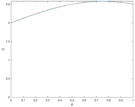
Figure 1.
Iterated approximations to the diffusivity function. (solid), (dash-dot) with , .
Given the cubic reaction term (16), is already a good approximation for the diffusivity function that leads to our exact solution for the phase field. Conversely, we may choose the diffusivity function to be and then exactly construct a reaction function that has the same generic properties as the canonical cubic function, but which exactly leads to the analytic solution for the phase field. From (9),
Figure 2 plots the cubic along with for .
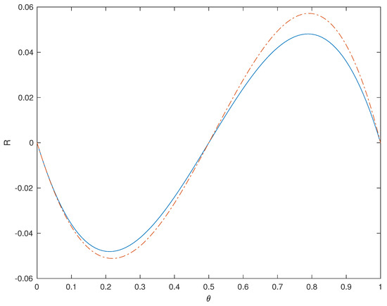
Figure 2.
Cubic reaction term R (solid). Exact matching partner (dash-dot) for with .
3. Interior Solutions for Slabs, Cylinders, and Spheres
In order to gain some understanding of the nature of the solutions, we consider interior solutions for slabs, cylinders, and spheres in dimensions , and 3 respectively. The four independent solutions will be trigonometric and hyperbolic functions (), Bessel and modified Bessel (), and spherical Bessel and modified spherical Bessel functions (). The solutions decrease uniformly in t towards . Even if the initial condition has in some significant sub-domain, the region where the source term is tends to stabilise phase .
Therefore, this global approach to Phase 0 should be controlled by the boundary conditions which may include, for example, ideal contact with the exterior pure phase at , or a Robin boundary condition for extraction of Phase 1.
The Case: .
In general coordinate systems with our adopted dimensionless variables, the simplified form of Equation (14) factorizes as:
where:
For radial flow within the ball , the Laplacian operator within (25) is . The two operator factors commute so (25) reduces simply to a system of two alternative second-order Helmholtz equations. The general solution of (25) in one, two, and three dimensions, with four free parameters , is:
Here, the spherical Bessel functions are defined simply as , , and .
For radial flows, the flux density of Phase 1 is:
For all values of n we impose zero flux at . For , considering the asymptotic behaviour of as shows that imposes two conditions on and :
These admit no non-trivial solutions, so . For alternatively imposing either or also gives two conditions on and similar to those above, which also imply .
For , imposing only implies a single condition:
However, is unbounded and hence unphysical in this context, unless:
which also ensures that . Again, the above two equations only admit the trivial solution .
For , only implies the condition:
As is finite, the case does admit physical solutions where and . We can eliminate this extra degree of freedom by imposing , to match the admissible solutions discussed above for and . This gives an extra condition on and :
so that again only is possible.
The boundary is in contact with pure Phase 0. Imposing , implies:
We have found in examples that the zero-flux boundary condition at will result in an inadmissible solution that is not positive semi-definite. However there is a solution that connects smoothly with an external slab of Phase 0, beginning at the boundary . Assuming , we deduce:
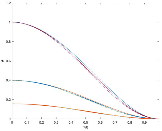
This has a sequence of solutions for . With , the first of these are and for , and 3 respectively, showing an significant increase with dimensionality. Higher values in the sequence of solutions for are found to produce unphysical solutions exhibiting negative values of u. With diffusivity and reaction term shown in Figure 1 and Figure 2 respectively, is given explicitly in terms of u as:
Although solutions for at different times are geometrically similar, this is not true for which is related to u by a nonlinear transformation. The solution for is depicted in Figure 3 for , . The solutions in dimensions are close after the three different domain radii are rescaled to the same value. The solutions depict an initial region in the neighbourhood of the origin, that consists predominantly of Phase 1, but is connected continuously through a thin mushy zone to a surrounding block of Phase 0, at . This mushy region is small enough to be stable under the Cahn–Hilliard evolution. Under the influence of the reaction, Phase 1 is normally stable, but its decay in this case is driven by the boundary conditions at , a boundary where the phase mixture is connected smoothly to an exterior bank of Phase 0. For example, from to , the exact radial solution on the interior of the sphere, depicted in Figure 3, has 90% of the initial volume of Phase 1 material exiting through the boundary, while the remainder undergoes a change to Phase 0 within the interior.
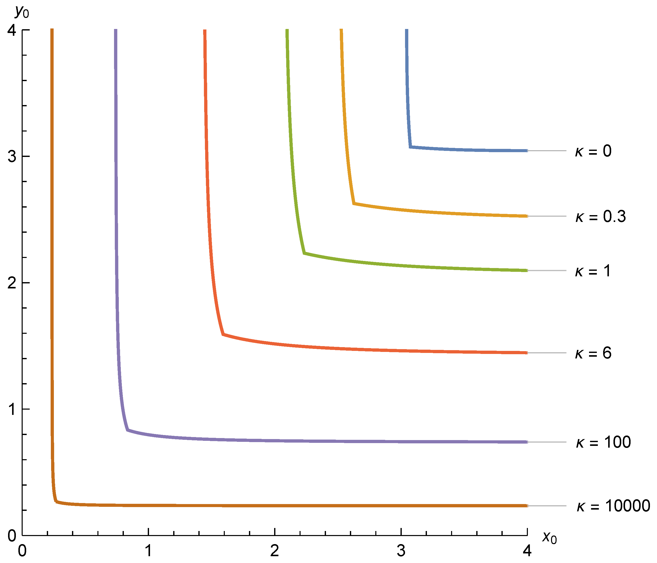
Unphysical solutions, with negative values of u, were found above for large values of . If one attempts to find the largest possible value of that produces a non-negative solution for a given , it soon becomes clear that for the class of solutions considered above, this corresponds to the first non-zero solution , of the above conditions shown in (33). This is a consequence of our solutions being a linear combination of one oscillatory, and one monotonically increasing function that take finite values at . As such, Figure 3 shows scaled examples of solutions with the maximum possible value of . Selecting smaller values of produces solutions with a non-zero negative slope at . Figure 4 shows variation of the maximum possible value as varies. In all cases as . The case does not produce valid solutions via our methods above, however the largest possible values of are obtained as , and Equation (33) approaches the following simple conditions in one, two, and three dimensions respectively:
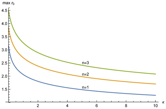
Figure 4.
Largest possible values of for various values of .
4. Interior Solutions for Rectangular Domains
Under idealised controlled boundary conditions on simple slab, cylindrical, or spherical domains, gives a maximum achievable diameter of the transition zone. However, there are many other solutions with finer sub-structure. This is consistent with the Cahn–Hilliard critical wavelength being of order 1, in dimensionless terms. The initial condition for may be any positive solution of the linear fourth order Helmholtz equation.
If we adopt Cartesian coordinates and restrict our attention to solutions that are identically zero on the boundaries , , the dimensionless form of Equation (14) with can be solved via the separation of variables. Setting we find two families of solutions where either:
If we focus on the latter case, and impose we find compatible values of :
Meanwhile must satisfy the differential equation:
provided that . This produces a solution similar to the first of (27):
The second form of above has the boundary condition imposed. Note that there is a maximum possible value of that will produce a non-negative function—hence, the situation is qualitatively similar to the examples of in various dimensions discussed in Section 3.
On the other hand, when we can define:
The corresponding solution then loses all periodicity:
The above form of will apply for all if:
that is, if is sufficiently small. When this condition is met there is no restriction on the size of implied by needing a non-negative solution .
In summary, if is sufficiently small we can choose to be as large as we want, however if shown above, there is some upper limit to the size of that will produce valid solutions. When all separable modes are accounted for, we can calculate the boundary separating feasible combinations of and from infeasible combinations. Figure 5 illustrates this boundary for various values of . Note that as the critical values of approach those indicated by the curve of Figure 4.
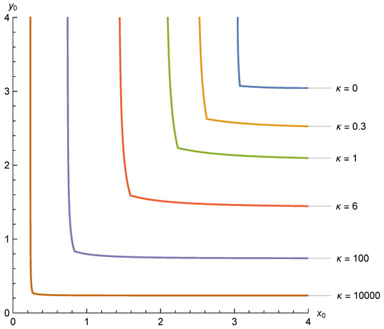
Figure 5.
Critical combinations of and separating the feasible rectangular solution region from the region where and in combination do not admit physical solutions.
When considering combinations of and that admit physical solutions, the eigenvalue corresponding to with = 0 is of primary importance as both and are non-negative. We view solutions with finer substructure as alterations of this solution that maintain the non-negativity of .
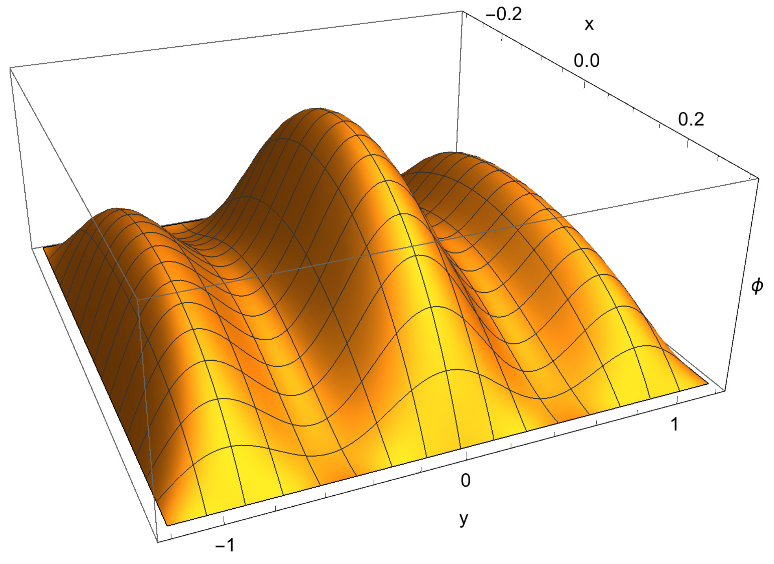
An example with a pronounced sub-structure is shown in Figure 6. Here, , , , and is proportional to where:

Figure 6.
A non-negative solution with , , and that exhibits a pronounced sub-structure.
From a brief exploration of the parameter space, it appears that solution regions with aspect ratios close to 1 typically allow little variation from , and tend to be unimodal. Solution regions that are more elongated can be multi-modal, and allow noticeable sub-structure as in the example of Figure 6.
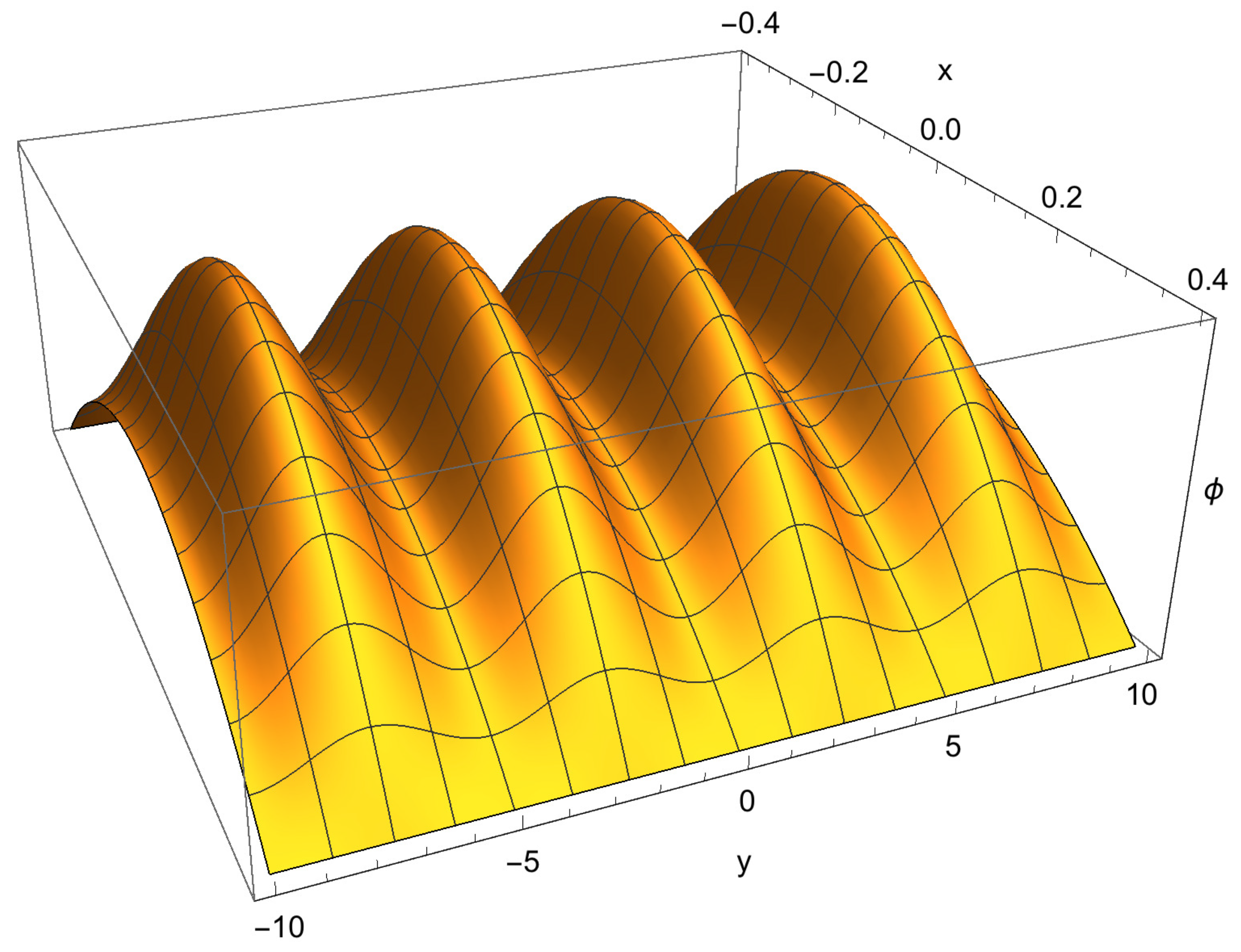
We can also consider rectangular solutions that are unbounded in a single direction, similar to the one-dimensional solution of Section 3. Let us begin by assuming that boundary conditions are applied to Equation (38) for . The eigenvalues of are still restricted by requiring a non-negative solution that remains finite as . Hence the separable solution must include , as its foundation. Equation (40) then gives a non-negative , provided that is not larger than the critical values illustrated in Figure 4 for . For values of significantly less than these critical values, we can produce noticeable sub-structure by adding other modes to this base solution while ensuring that remains non-negative and finite. Figure 7 shows one such solution with and . It is proportional to , with . Here is given by (40) with , , and and replaced by and as given by Equation (26), respectively. is also given by (40) with , , but with and replaced by:

Figure 7.
A non-negative solution , periodic in the y direction with , and .
It is also possible to obtain a rectangular unbounded solution by first applying on the solutions of . Seeking a finite non-negative value of X(x) again supports the conclusion that no solutions are possible for values greater than those indicated by the curve of Figure 4.
In summary, our consideration of solutions interior to a rectangular region is compatible with the maximal values of derived in Section 3, and shows that exact solutions with varied substructures are possible.
5. Energy Formulation
Let us consider the original equation in (13),
In this section we assume is an open, bounded subset of with a smooth boundary (). Conforming to Section 3, so that the fourth-order diffusion term, which dominates at high wave numbers, has negative spectrum, generating a diffusion process that propagates forward in time. With no loss of generality, we set . Equation (46) is a fourth-order quasi-linear equation in divergence form. Although the fourth-order term can be written as , that is, the cascade of two symmetric second-order operators with , it turns out that is not symmetric and therefore there is no associated energy functional of which is the first variation. We introduce the flux potential variable defined as where , . We also assume is smooth and strictly positive, implying that is 1-1 and globally invertible. By substituting into Equation (46) we obtain:
Here we have defined and . With some abuse of notation—and to keep the notation consistent with the previous sections—in what follows we drop tildas.
We remark that the approach leading to writing Equation (47) is essentially the substitution method largely employed in the theory of porous medium equations [34]. In soil physics, the variable u is well known as the matric flux potential [19,20]. It is relevant to the physics of the flow since is the soil–water flux driven by the intrinsic capillary action of the soil matrix, without gravity.
By exploiting the linear structure of the right hand side of (47) the investigation of existence results of the solution becomes more transparent. Let us consider the static problem when obtained by setting in Equation (47). Although in this paper we are mainly concerned with time-dependent problems, the static regime is of interest as the solutions of it represent ground-state configurations for the physical system. Eliminating time-dependence in (47) yields:
Equation (48) is obtained as the linear combination of symmetric operators and it does have a variational structure. Indeed, it coincides with the first variation of the functional:
where . The derivation of (48) from (49) has been performed formally. Under the regularity assumptions on and if verifies suitable growth conditions (here unspecified), the derivation of the Euler–Lagrange equation (48) is exact in . The subspace of -Sobolev functions with higher-order energy norm (where denotes the Lebesgue space of square-integrable functions) with zero boundary conditions for u and , where is the outward normal to . Non-homogeneous boundary conditions are incorporated by introducing , the set containing all the -functions u such that , with representing the boundary datum.
By exploiting the variational structure of the problem, one may look for solutions to (48) as the critical points of (49) and vice-versa. The nature of the critical points of I is determined by the sign of b as well as the shape of . As an example, when and with , the Lax–Milgram lemma ensures that there exists a unique solution of Equation (48), denoted with , and that is the unique minimizer of in . Furthermore, when , by elliptic bootstrapping we recover that is the classical (indeed in ) solution to Equation (48). From the knowledge of the solution to Equation (48), one is able to recover information on a function which solves the original Equation (46) in the static regime (i.e., ) by simply plugging into Equation (46). In more physically relevant situations represents a competing energy contribution usually in the form of a non-negative multi-well function in the variable u. When is a non-convex non-negative polynomial it may still be possible to ensure the existence (although not the uniqueness) of the solution to the minimum problem for possibly in a subset of and characterize as a solution to Equation (48). Instead, when and with we have genuine competition in the summands of the energy I and in turn I may fail to be positive-definite. Under these circumstances, solutions to Equation (48) correspond to various critical points of I including saddles or more intricate situations. In those cases, existence theorems should be investigated by methods possibly based on min-max principles.
An alternative approach (e.g., [15,16]) is to express the phase flux density as being proportional to the negative gradient of a chemical potential energy density that is itself the variational derivative of a total internal energy functional. This comes about because the drift velocity of the mobile particles of Phase 1 quickly reaches a terminal velocity that enables the driving gradient of chemical potential energy to be balanced by a mechanical resistance force that is proportional to velocity and in the opposite direction. The new element that we need here to justify the non-standard Equation (6) is that the variational derivative is taken with respect to the flux potential u, rather than the phase variable . Then we choose:
In this set-up, must be regarded as an externally driven Phase 1 production term that assists relaxation towards the stable fixed points.
6. Conclusions
A nonclassical symmetry reduction has led to some exact positive solutions for multi-dimensional nonlinear reaction–diffusion equations with both fourth-order diffusion and second-order backward diffusion. In all likelihood, these are the only known exact solutions for equations of the Allen–Cahn–Hilliard type that have meaningful boundary conditions. The presented solutions have a zero flux and a zero gradient at one central boundary point, plus a prescribed value, representing a pure phase, as well asa zero gradient at the other boundary. The initial condition has the phase field taking the value at . Even though Phase 1 is stabilised by the reaction term, the boundary conditions force the solution to have the system uniformly approaching Phase 0. An interior cylindrical or spherical inclusion with a mixed phase could not withstand the inward advance of Phase 0 from the outer boundary.
Structured phase domain patterns have been seen in numerical solutions of the Cahn–Hilliard equation (e.g., [35]). Some exact solutions with pronounced sub-structure have been produced here too. Since the exact solution involves a general solution of the fourth-order linear Helmholtz equation for the flux potential, it is possible that more complex patterns could be incorporated in the future. Any solution of the fourth-order Helmholtz equation can be used in this method, even those that apply in more complicated asymmetric domains.
We remark the approach based on the Helmholtz substitution adds additional structure to the model in terms of a variational principle as the by-product of symmetry and linearity. Although the thorough investigation of the relation between the non-linear model in the unknown variable and the transformed model in u is not the scope of the present contribution, in Section 5 some insight is provided for some special situations. The construction used here became possible because of a nonclassical symmetry that applies when the nonlinear diffusivity and the nonlinear reaction term together obey a single relationship. Then an additional constraint
added to the governing PDE, results in an integrable system. Reduction of variables then results in the linear fourth-order Helmholtz equation. In that sense, the original multidimensional nonlinear scalar PDE is partially integrable because one additional constraint leads to a linear PDE with one fewer independent variables. It remains to be discovered whether nonclassical symmetry classification can unearth other semi-integrable PDEs—possibly defined by different fourth-order non-linear operators—in this way, and more generally, how compatible constraints may be selected.
Acknowledgments
D. Gallage gratefully acknowledges the support of a La Trobe University postgraduate scholarship, while on study leave from the University of Colombo. P. Cesana is partially supported by the JSPS Research Category Grant-in-Aid for Young Scientists (B) 16K21213 and is a member of the GNAMPA.
Author Contributions
Philip Broadbridge conceived of the project and set up the mathematical models, Dimetre Triadis and Dilruk Gallage did most of the calculations and Pierluigi Cesana provided the formal existence and energy analysis.
Conflicts of Interest
The authors declare no conflict of interest.
References
- Wang, Y.U.; Jin, Y.M.; Cuitiño, A.M.; Khachaturyan, A.G. Nanoscale phase field microelasticity theory of dislocations: Model and 3D simulations. Acta Mater. 2001, 49, 1847–1857. [Google Scholar] [CrossRef]
- Green, H.S.; Hurst, C.A. Order-Disorder Phenomena; Interscience: London, UK, 1964. [Google Scholar]
- Yu, L.; Ding, G.L.; Reye, J.; Ojha, S.N.; Tewari, S.N. Mushy Zone Morphology during Directional Solidi Cation of Pb-5.8 Wt Pct Sb Alloy. Metall. Mater. Trans. A Phys. Metall. Mater. Sci. 2000, 31, 2275–2285. [Google Scholar] [CrossRef]
- Cahn, J.W.; Hilliard, J.E. Free energy of a nonuniform system. I. Interfacial free energy. J. Chem. Phys. 1958, 28, 258–267. [Google Scholar] [CrossRef]
- Allen, S.M.; Cahn, J.W. A macroscopic theory for antiphase boundary motion and its application to antiphase domain coarsening. Acta Metall. 1979, 27, 1085–1095. [Google Scholar] [CrossRef]
- Gurtin, M.E. Generalized Ginzburg-Landau and Cahn-Hilliard Equations based on a microforce balance. Physica D: Nonlinear Phenomena 1996, 92, 178–192. [Google Scholar] [CrossRef]
- Caginalp, G. The dynamics of a conserved phase field system: Stefan-like, Hele-Shaw, and Cahn-Hilliard models as asymptotic limits. IMA J. Appl. Math. 1990, 44, 77–94. [Google Scholar] [CrossRef]
- Jones, J.A. Derivation and analysis of phase field models of thermal alloys. Ann. Phys. 1995, 237, 66–107. [Google Scholar]
- Novick-Cohen, A. The Cahn-Hilliard Equation. In Handbook of Differential Equations. IV Evolutionary Partial Differential Equations; Dafermos, C., Pokorny, M., Eds.; Elsevier: Amsterdam, The Netherlands, 2008; pp. 201–228. [Google Scholar]
- Kim, J.; Lee, S.; Choi, Y.; Lee, S.-M.; Jeong, D. Basic Principles and Practical Applications of the Cahn-Hilliard Equation. Math. Probl. Eng. 2016, 2016, 9532608. [Google Scholar] [CrossRef]
- Landau, L.D.; Khalatnikov, I.M. On the theory of superconductivity. In Collected Papers of L.D. Landau; Ter Haar, D., Ed.; Pergamon: Oxford, UK, 1965. [Google Scholar]
- Skellam, J.G. The formulation and interpretation of mathematical models of diffusionary processes in population biology. In The Mathematical Theory of the Dynamics of Biological Populations; Bartlett, M.S., Hiorns, R.W., Eds.; Academic Press: New York, NY, USA, 1973; pp. 63–85. [Google Scholar]
- Broadbridge, P.; Bradshaw, B.H.; Fulford, G.R.; Aldis, G.K. Huxley and Fisher Equations for Gene Propagation: An Exact Solution. Anziam J. 2002, 44, 11–20. [Google Scholar] [CrossRef]
- Bradshaw-Hajek, B.H.; Broadbridge, P. A robust cubic reaction-diffusion system for gene propagation. Math. Comput. Model. 2004, 39, 1151–1163. [Google Scholar] [CrossRef]
- Ulusoy, S. A new family of higher order nonlinear degenerate parabolic equations. Nonlinearity 2007, 20, 685–712. [Google Scholar] [CrossRef]
- Karali, G.; Katsoulakis, M.A. The role of multiple microscopic mechanisms in cluster interface evolution. J. Differ. Equ. 2007, 235, 418–438. [Google Scholar] [CrossRef]
- Galaktionov, V.A.; Svirshchevskii, S.R. Exact Solutions and Invariant Subspaces of Nonlinear Partial Differential Equations in Mechanics and Physics; Chapman & Hall/CRC: Boca Raton, FL, USA, 2007. [Google Scholar]
- Cherniha, R.; Myroniuk, L. Lie symmetries and exact solutions of a class of thin film equations. J. Phys. Math. 2010, 2. [Google Scholar] [CrossRef]
- Raats, P.A.C. Analytic solutions of a simplified flow equation. Trans. ASAE 1976, 19, 683–689. [Google Scholar] [CrossRef]
- Philip, J.R. The scattering analog for infiltration in porous media. Rev. Geophys. 1989, 27, 431–448. [Google Scholar] [CrossRef]
- Ovsiannikov, L.V. Group Analysis of Differential Equations; Academic Press: New York, NY, USA, 1982. [Google Scholar]
- Fushchych, W.I. How to extend symmetry of differential equations? In Symmetry and Solutions of Nonlinear Equations of Mathematical Physics; Institute of Mathematics Ukrainian Academy of Sciences: Kyiv, Ukraine, 1987; pp. 4–16. [Google Scholar]
- Bluman, G.W.; Cole, J.D. The general similarity solution of the heat equation. J. Math. Mech. 1969, 18, 1025–1042. [Google Scholar]
- Mansfield, E. The nonclassical group analysis of the heat equation. J. Math. Anal. Appl. 1999, 231, 526–542. [Google Scholar] [CrossRef]
- Arrigo, D.J.; Hill, J.M.; Broadbridge, P. Nonclassical symmetry reductions of the linear diffusion equation with a nonlinear source. IMA J. Appl. Math. 1994, 52, 1–24. [Google Scholar] [CrossRef]
- Clarkson, P.A.C.; Mansfield, E.L. Symmetry reductions and exact solutions of a class of nonlinear heat equation. Physica D 1993, 70, 250–288. [Google Scholar] [CrossRef]
- Cherniha, R.; Davydovych, V. Nonlinear Reaction-Diffusion Systems. Conditional Symmetry, Exact Solutions and Their Applications in Biology; Springer: Berlin, Germany, 2017. [Google Scholar]
- Goard, J.; Broadbridge, P. Nonclassical symmetry analysis of nonlinear reaction-diffusion equations in two spatial dimensions. Nonlinear Anal. Theory Methods Appl. 1996, 26, 735–754. [Google Scholar] [CrossRef]
- Kirchhoff, G. Vorlesungen über die Theorie der Wärme; B. G. Teubner: Leipzig, Germany, 1894. [Google Scholar]
- Broadbridge, P.; Bradshaw-Hajek, B.H.; Triadis, D. Exact non-classical symmetry solutions of Arrhenius reaction-diffusion. Proc. R. Soc. Lond. A 2015, 471. [Google Scholar] [CrossRef]
- Broadbridge, P.; Daly, E.; Goard, J. Exact solutions of the Richards equation with nonlinear plant-root extraction. Water Resour. Res. 2017, 53, 9679–9691. [Google Scholar] [CrossRef]
- Broadbridge, P.; Bradshaw-Hajek, B. Exact solutions for logistic reaction-diffusion in biology. Z. Angew. Math. Phys. 2016, 67, 93–105. [Google Scholar] [CrossRef]
- Tehseen, N.; Broadbridge, P. Classification of Fourth Order Diffusion Equations with Increasing Entropy. Entropy 2012, 14, 1127–1139. [Google Scholar] [CrossRef]
- Vázquez, J.L. The Porous Medium Equation; Clarendon Press: Oxford, UK, 2006. [Google Scholar]
- Liu, Q.-X.; Doelman, A.; Rottschäfer, V.; de Jager, M.; Herman, P.M.J.; Rietkerk, M.; van de Koppel, J. Phase separation explains a new class of self-organized spatial patterns in ecological systems. Proc. Natl. Acad. Sci. USA 2013, 110, 11905–11910. [Google Scholar] [CrossRef] [PubMed]

© 2018 by the authors. Licensee MDPI, Basel, Switzerland. This article is an open access article distributed under the terms and conditions of the Creative Commons Attribution (CC BY) license (http://creativecommons.org/licenses/by/4.0/).