Abstract
Modern 5G networks offer a large space for innovation and a completely new approach to addressing network functioning. A fixed spectrum assignment policy is a significant limitation of today’s wireless communication network practice and is to be replaced by a completely new approach called dynamic spectrum access (DSA). However, there is no general agreement on the organization of the DSA. Some studies suggest that open access market can be inspired by the electricity or financial markets. It allows to treat operators with region coverage as investors entering the market and trading the spectra on an on-demand basis. Because investors operate in both the financial markets and the markets for spectra, new interference between both markets emerges. Our paper shows how the risk-free rate of return stemming from the financial markets influences the techno-economic properties of the network. We show that, for low risk-free returns, the spectrum market becomes oversupplied, which keeps service prices very low and spectrum trading volumes large. In contrast, if risk-free returns are high, then spectrum trading volumes decline and the market becomes price sensitive; in other words, economic rules begin to work better.
1. Introduction
The development of human society is connected with the rapid growth of data, which doubles every two years according to a recent study of IDC iView "Extracting Value from Chaos" sponsored by EMC Corporation (Hopkinton, MA, U.S.) [1]. This fact increases the demand for growing data volume transfers as a result of the increasing interconnectivity in society and the larger number of autonomous intelligent devices with communication abilities. Currently, telecommunication services cover between 3 and 6 percent of the gross domestic product of national economies and have become an indispensable factor of further development. The importance of the telecommunication sector is evident from the oft-declared empirical evidence on the causal relationship between telecommunication services and economic growth (e.g., by [2,3,4]). In contrast, the traditional command-and-control spectrum management based on exclusive access to the frequency spectrum by licensed operators becomes a serious limiting factor [5]. Licensed operators are not able to permanently utilize the entire frequency band, leading to temporally inefficient spectrum utilization. The solution to the problem is Dynamic Spectrum Access (DSA), which is a set of innovative spectrum management schemes that allows for more efficient spectrum utilization based on Cognitive Radio (CR) technology. Hossain et al. [6] describe the economic model behind the DSA as follows. Primary operators (POs) participate in auctions on the primary market to lease the frequency spectra licenses needed to provide the primary service. Then, POs that seek to dispose of unused parts of the licensed spectrum enter a spectrum secondary market and lease them temporarily to secondary operators (SOs) through various trading schemes that merge the technological and economic aspects of the topic (We note that our notion of “primary” and “secondary” spectrum providers must be distinguished from similar terms often associated with users themselves (in our case, end users) [7]). The chosen trading scheme should take into account both the contradictory goals of independent users and the existence of the artificial intelligence disseminated across the entire network [8]. Therefore, DSA technology enables an increase in spectrum utilization and, at the same time, improves the network’s economy, which satisfies the inflow of the additional financial sources needed to expand and modernize the existing network.
The paper is organized as follows. In Section 2, we provide a brief overview of the ideas that motivate the creation of an open access market on the basis of principles in financial markets. An agent-based model is proposed in Section 3. In Section 4, we present an analysis of the model’s parameter sensitivity. A detailed analysis of the risk-free returns’ impacts on network techno-economic properties is provided in Section 5. Section 6 draws some important conclusions.
2. Frequency Spectrum Market as a Form of Financial Market
To date, various trading schemes for the secondary spectrum market have been proposed. Evci and Fino [9], in their very first study on spectrum management, define spectrum trading as a substantial part of spectrum management. They first identify the difficulties and weaknesses of the traded spectrum pricing, point to the complexity of the topic, and express their skepticism regarding application of optimization techniques. Hossain et al. [6] more deeply analyze the spectrum pricing phenomena. They show that sellers (POs) maximize their profits and, on the other side, SOs maximize the utility derived from their spectrum use. Both goals are contradictory because sellers are interested in high selling prices and leasers avoid them. Similar contradictory goals result from the fact that an increase in the frequency spectra used by SOs causes an increase in their overall utility, whereas POs may suffer from spectrum shortage. These contradictions are to be considered if defining the key properties in the PO–SO trade interaction. Notwithstanding this issue, it seems that the neoclassical economic methods accommodated for the DSA, as proposed by Nyiato et al. [10], are not entirely applicable. (Nyiato et al. [10] adapted neoclassical microeconomics methods for the DSA conditions. They derived demand and supply functions and identified the equilibria where the demand and supply of the spectra are balanced perfectly. They extended their analysis also through the assumption of the existence of a monopoly and collusive oligopoly on the side of the POs. In contrast, we mention that neoclassical theory was never applied in its pure form in research on the DSA, despite its mathematical elegance.) However, there remains the concept of profit-maximizing POs and utility-maximizing SOs entering the auction through various channels or adopting the bargaining techniques currently prevailing in the DSA. Both methods are based on a compromise agreement between seller and leaser; therefore, they reduce the contradictions in the primary goals of both trading partners. In contrast, these trading schemes concretely eventuate PO–SO matching and apply to small groups of trading partners or deals involving a longer lease period.
This rather new situation means open access to the markets. According to Cramton and Doyle [11], the barriers to entry to the market dealing with network capacities are removed, and anyone can gain access to mobile communication services at nondiscriminatory prices. In contrast, because network capacities are scarce, their pricing satisfies the returns to owners, and prices economically regulate the network. Under these conditions, the self-regulatory properties of the network become crucial.
The best example of market efficiency is provided by the capital markets. Fama [12,13] asserts that all real-time stock prices reflect the information available to the public, which prevents some investors from gaining exclusive returns at the expense of others. At the same time, the evolution of stock prices serves as the main source of concentrated information on the issuer’s economic condition, which can attract or discourage investors. This has a direct impact on the ability of the firm to acquire external financing on the basis of its performance. The shares of companies in bankruptcy are of negligible value, whereas blue chips are the best-priced companies with priority access to external resources.
The properties of the capital markets, as previously mentioned, motivated organizers of other types of markets to mimic the capital markets. Currently, financial instruments are available in commodities markets that have properties fully in line with the capital markets. A similar situation prevails in the electricity markets. Various investors lease and sell power plant capacity through various financial instruments (forwards, options), thus increasing market efficiency. According to Cramton and Doyle [11], the electricity market arrangement organization provides ideas and solutions that are directly applicable in the open access markets with frequency spectra.
In their proposal on the open market organization, Cramton and Doyle [11] distinguish POs, SOs (e.g., mobile network virtual operators (MVNO) and operators with regional importance), and end users. Network capacities should be traded in the wholesale (i.e., POs, SOs) and retail markets (service demand by end users). They also propose a forward market, enabling trade with forwards for network capacities. The main motivation for establishing the forward market should be its stabilizing impact on retail markets.
The main goal of our research is to simulate the functioning of the forward and retail markets using the traditional modeling approach applied in previous spectrum trading studies. For a more detailed analysis, we decide to model the behavior at the basic granularity level, i.e., interactions among a single PO, a few SOs, and a larger number of end users. The basic research question is: How large is the impact of the risk-free rate of return on the techno-economic properties of the entire network? At the same time, we are interested in answering the question of whether SOs are interested in investing in forwards, even if the risk-free rate of return is extraordinary high or extraordinary low. A further question is whether returns of the SOs exceed the long-term risk-free rate of return, even if they are investing in risky assets (i.e., forwards), as assumed by the author of Portfolio theory, Harry Markowitz [14]. In contrast, based on the conclusions of the separation theorem formulated in the theory of investments by James Tobin [15], the increase in the risk-free rate of return should imply an increase in spectrum retail market returns.
3. Model Preliminaries
Given the turbulent recent research, it is relatively straightforward to imagine the technical aspects of 5G (i.e., the forthcoming employment of the carrier-aggregation feature, multi-homing, network switching, and others). Instead, in our model, we more strongly emphasize the economic factors that influence the existence of secondary 5G spectrum markets in general. However, to accomplish that, we need to relax the technical platform of our model to the dedicated level that still correctly models operator and end user behavior. Thus, we decided to model the conventional LTE system with no carrier aggregation future, but allow for end users to perform network switching. The network switching feature allows end users to dynamically switch providers on the basis of instantaneous conditions at a small timescale (i.e., scale on the order of seconds). The switching is performed entirely on the end user terminal and, thus, no operator support is required. Google recently introduced U.S. pilot Project Fi where Google acts as the SO that aggregates three 4G LTE network operators (Sprint, T-Mobile and regional carrier US Cellular) through dynamic switching of network SIM profiles, which has an average switching time of 8.8 s and a potential lower bound switching time of 1.5 s [16]. Project Fi intelligently connects the end users to the operator’s network and seamlessly moves them between the partner LTE networks for delivering the most reliable and fastest available wireless service at the cost of reasonable price. Project Fi may be an important step towards meeting the 5G requirements of ultra-high reliability and very low latency while taking economic considerations into account [17,18]. In line with the promising Project Fi implementation, there exist several theoretical studies evaluating the performance of the network switching mechanism in 5G networks. The authors in [19,20] suggest that the network-switching mechanism improves spectrum allocation efficiency on a dynamic basis and thus has the potential to serve as the promising solution in the forthcoming 5G networks. The underlying idea supporting this expectation is the application of the Multipath Transmission Control Protocol (MPTCP), which is already implemented by Apple in its operating system (iOS7) [21]. MPTCP is capable of switching the user connection autonomously from one operator to another in real-time, which further simplifies the network switching application. Thus, assuming the network switching feature in our model seems reasonable.
We model the end user’s decision using the conventional utility concept, which captures both the signal quality and the price of the service. In contrast, the intelligence employed on the operator side allows for adjustment of the volume of frequency resources to be leased on the DSA (i.e., forward market), which is the foundational concept of the DSA feature. Both mechanisms (i.e., DSA and network switching) are expected to contribute to the increased spectrum efficiency of 5G networks [22].
Within the modeling framework, we follow the conclusions presented in [23] and, thus, propose a hierarchical spectrum market structure with the following agents: (i) primary spectrum (wireless service) operators (i.e., a.k.a. POs); (ii) secondary spectrum (wireless service) operators (i.e., a.k.a. SOs); and (iii) end users. To analyze the impacts of the risk-free rates on the secondary spectrum market, an agent-based model has been proposed. The market model consists of a forward (i.e., wholesale) market, where SOs lease the frequency spectrum forwards from the PO one year ahead, and a retail market intermediates trades between SOs and end users and operates in real-time. Dynamic spectrum distribution occurring on the wholesale market forms the underlying concept of DSA markets. Forward trades run once a day and retail trades run once an hour (i.e., 24 times a day). The basic market scheme that illustrates its organization structure is given in Figure 1. In our model, we stress our intention for the existence of the spectrum secondary market and retail market and leave the primary market interactions (e.g., interactions among FCC and POs) for a future discussion.
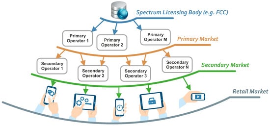
Figure 1.
Primary, secondary, and retail spectrum markets.
Network Topology
We model the existence of the PO given a base-transceiver station (BTS) in the investigated region. Following the concept of open access markets, the available frequency resource blocks (RBs) are subject to the trading between a dedicated PO and a set of SOs. Note that because of their nature, SOs do not have a unique infrastructure and rely on the current PO infrastructure (i.e., infrastructure sharing). The SOs optimize the volume of frequency RBs purchased on the secondary spectrum access using the Roth-Erev algorithm (description given in the following sections). These frequency resources are subsequently used on the retail market to accommodate end user demand.
The entire spectrum trading process on the retail market is initiated by an end user who expresses the desire to use a service by broadcasting a price request to SOs over a designated signaling channel. This initial connection can be considered analogous to the operation of either a domain name server (DNS) or dynamic host configuration protocol (DHCP) in computer engineering. SOs with a non-zero amount of free RBs respond to the end user with their price offers. Using the prices obtained from the operators and the corresponding utilities, the end user makes a spectrum trading decision that consists of two phases: selecting the best offer (the winning SO) and deciding on whether to accept the bidding price. We consider an interference-free system in which the spectrum allocations are valid throughout the region and no two sessions can occupy the same frequency band. In other words, at each RB in the frequency spectrum, at most one end user-SO pair communicates at a time. The relevance of such a system model was previously discussed in, for example, [24].
An example of the secondary spectrum market network with corresponding agents is depicted in Figure 2. In following, we provide a more detailed description of the agents’ behavior.
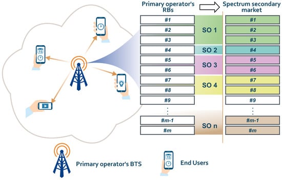
Figure 2.
Schematic diagram of the network model with PO, set of SOs and end users.
4. Agent-Based Model of Open Access Market
4.1. Forward Market
The forward market allows POs to lease dedicated spectra to SOs while keeping the forward price constant for the entire simulation. This resembles the typical idea of dynamic spectrum distribution among the entities in the DSA market [25]. This strategy satisfies stabilization of the market and is motivated by the analogous strategies of central banks offering loans to commercial banks at a fixed discount rate or keeping fixed the exchange rates of the domestic currency. Then, the discount rate or the exchange rate serves as a signal for market participants on how to form their own strategies and expectations. Therefore, we also assume that a fixed bid price in the forward market will act as an intermediary in stabilizing the retail market.
Let represent a set of SOs, where each SO has constant monetary budget I every day. The strategy of the i-th SO consists of investing proportion of its budget I in daily forwards leased from the PO and the rest in risk-free instruments. The trade runs once a day. (Treasury bills are usually considered risk-free investments.)
The number of frequency RBs leased by i-th SO is calculated as follows
where denotes the floor function. Then, the total (daily) profit of the i-th SO is given as
where r is a risk-free return rate, represents the set of real one-hour end user connections to the i-th SO, is the unit price paid by the j-th end user to the i-th SO, and is the number of one-hour forwards that the i-th SO leased one year ago.
We assume that SOs learn how to maximize their profits by choosing their optimal investment strategy. Therefore, in line with forwards modeling in the electricity market as proposed by [26], the Roth-Erev reinforcement learning algorithm [27] has been applied. The underlying idea behind the application of Roth-Erev algorithm would be putting in place a system that would not allow oversupply (and therefore wastage of spectrum) and at the same time under-supply of the frequency resources. The aim of the system is to find the strategies to be learned based on the agent’s interactions that avoid this outcome. Information about agent’s own experiences are memorized for a period of time but some of them are forgotten at certain time horizons. To accomplish that, different combinations of the two learning parameter (forgetting and experience) in the Roth-Erev algorithm are used. Analogous concept can be seen when the agents in the financial market try to optimize the information about market history stored in their memory to derive forecast of the future market development [25].
The algorithm uses the propensity function that maps the strategy space onto the set of real positive numbers
with the dynamics defined as follows. In the first simulation round
else
where represents the current propensity if the i-th SO chooses strategy j, superscript denotes the next period, is the recency parameter, is the unity-based normalized income gained by playing the k-th strategy, (Unity-based normalization is used to transform the data to the range, i.e., ) and is an experimentation parameter.
SO i chooses its j-th strategy in time t with the probability
The sequence of the actions performed by each SO in leasing the frequency spectrum on the forward market is given in Algorithm 1.
| Algorithm 1 Leasing process in the forward market |
|
The PO profit in time t is defined as current income from the forwards leased to the SOs:
4.2. Retail Market
We recognize two different agents acting on the retail market: end users (i.e., responsible for the selection of SOs) and SOs (i.e., responsible for competitive pricing). Their mutual interactions are provided in this section.
4.2.1. End User Interactions
We employ the micro-economic concept using the end user utility determined by its perception of quality of service (QoS) [28]. We assume that the only factor determining QoS is the distance between the end user and the operator (This is a reasonable assumption as long as end user uniformity in the region is assumed and, at the same time, equal transmission power exists across all RBs). Then, the utility of j-th end user is defined as
where is the distance between the j-th end user and the BTS and are the parameters that define the exact shape of the utility function. The relevance of the utility selection in the model was discussed in our previous work [25] and we refer the interested reader therein.
In addition to the QoS, the end user considers the price paid for a service. Hence, according to [6], we specify an acceptance probability function for the j-th end user considering the price bid of the i-th SO. The acceptance probability function is as follows
where is the bid price of the i-th SO and and are the shaping parameters.
In the selection process, the j-th end user chooses the i-th SO, allocating him or her the highest acceptance probability. In our system model, the main constraint is the obvious limited capacity of the network. Clearly, operators possess a limited number of available frequency RBs. Thus, it seems inevitable to jointly measure the utility of the end users with the role of pricing from the operators’ perspective. Here, the perception of the service for end users is remarkably different if the price is changed. In practice, end users are satisfied with the service if both quality and price paid are considered acceptable [24].
During the simulation, the end user inhabits one of the three internal states: IDLE, ACTIVE, or CONNECTED. The end user who is not interested in connecting to the network is inactive in the state IDLE, but at each time instant can be randomly switched to the ACTIVE state with a probability . The active end user decides to connect to one of the SOs on the basis of the estimated . Thus, the end user sends a request to each SO and either selects the one with the highest and switches to the CONNECTED state or returns to the IDLE state. Moreover, the connected end user can remain in the CONNECTED state with probability or disconnect and switch to the IDLE state with probability . Transitions between different end user states and their decision-making processes are given in Algorithm 2.
| Algorithm 2 Decision process of the end user repeated in each time step |
|
4.2.2. SO Pricing Adjustment
SOs sell their frequency RBs previously leased in the forward market to end users. In line with other studies (e.g., [29]), the i-th SO maximizes its profit (see (2)) by searching for the optimal bid price strategy that applies the linear reward-inaction algorithm.
At each instant hour, the i-th SO randomly selects bid price and sells the hired network resources to end users accepting its bid price. At the start of the simulation, the probability distribution of the bid prices is uniform (i.e., ), and is iteratively updated in the following simulation steps
where is the learning parameter (). The learning process stops when there is negligible increment in the probability vector.
The trade action of the SO consists of two different stages: (a) request processing and (b) retail pricing. All requests received from end users are saved. The SO recognizes three types of requests: price, connection, and removal. If there is a free available RB , an actual price offer for a frequency RB is sent to the requesting end user in response to the price request. The SO’s request processing is described in Algorithm 3. The retail pricing process follows the linear reward-inaction algorithm previously described.
| Algorithm 3 SO request processing |
|
5. Parameter Sensitivity
The proposed model contains a large number of different parameters that influence the agent’s behavior. In general, agent-based models are sensitive to parameter settings, which means that different parameter values can lead to different results. In contrast, the model outputs can be quite robust against the variations in other parameters [30]. Several approaches to studying parameter sensitivity have been developed [31] to understand the features of agent-based modeling. Because we need to consider the impacts of many parameters, we chose global sensitivity analysis, which is based on the regression wherein random samples are drawn from the parameter space as introduced in Table 1.

Table 1.
Parameters sensitivity analysis settings.
For each random draw, we ran a simulation and recorded the simulation outputs describing the techno–economical properties of the secondary spectrum market. After performing 500 simulations of 1000 simulation days each, we ran a linear regression with the right-hand side explanatory variables given by the parameters in consideration. Each regressed variable explains particular network characteristics: average retail price , average daily profit of one SO, average spectrum utilization , average daily number of frequency RBs leased by one SO , average propensity to invest in the secondary spectrum market , average number of connections per day , and average PO profit .
Using the simulation results, regression coefficients were estimated and the results are provided in Table 2. Numerous SOs n are shown to have a statistically significant effect only on the average profit of the PO . If the number of SOs increases by 1, then the daily profit of the PO increases by 2460 monetary units because of stronger demand in the forward market caused by the larger number of SOs. The impact of this parameter on the other explanatory variables is not significant and may result from the average propensity to invest , which is rather surprising. This finding indicates that we did not collect empirical evidence that shows that increasing competition on the side of the SOs significantly changes their investment behavior. In contrast, SOs’ propensity to invest grows if the number of end users of the (total addressable market) also grows. Further, we conclude that the change in SO behavior is rather small; hence, the impact of the increase in the is not intermediated by the significant increase in the number of frequency RBs leased by SOs . The probability of disconnection does not have a significant effect on the analyzed network indicators.
Table 2.
Parameter sensitivity of the model.
The SO’s budget I induces the average number of leased frequency RBs , PO profit , and average SO profit . The effect of the Roth-Erev algorithm parameters is also studied. Both parameters and statistically significantly affect SO behavior . Parameter affects the profit of PO . The last analyzed parameter is the forward price , which influences only the number of leased frequency RBs .
Agent-based simulation is slower process compared with the deterministic optimization because it more resembles stochastic optimization in variable landscape. The decisions and bursty activities of agents may include many consecutive revisions of the previous tendencies, thus the results are less straightforward which seems better suited for the realistic situations. The complexity of the search, and therefore the speed of convergence are not universal, but closely related to the number of options that the agent must deal with before making a decision. Thus, the convergence speed of the algorithm is the function of the agent’s strategy space and we can reduce/enlarge it based on the model’s (operator’s) requirements.
For the illustration we present the convergence properties of the Roth-Erev algorithm for the given parameters (, ) used throughout the simulation scope in Figure 3.
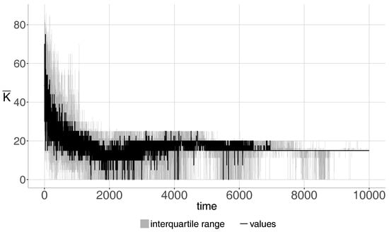
Figure 3.
Convergence properties of the Roth-Erev algorithm with different strategies, eventually converging to the pure strategy.
Initially, the SO experiments with the number of leased RBs, which is actually the fundamental idea of the class of reinforcement learning strategies. However, as the system evolves over the time, the strategy space of the SO is collapsed to the pure strategy action.
6. Simulation Results
We assume that the market for the frequency spectrum is efficient and reflects the shocks originating in the financial markets. The response of the techno-economic properties of the telecommunication network to the returns of the risk-free assets is presented in the following analysis.
The exploratory simulation is run ten times with the same parameter settings. One year consists of 360 days and one day consists of 24 h. One hour represents the minimum connection length. The parameters that characterize the end users’ decision process are set to make the end users quality and price sensitive. This reflect the real behavior of the consumers, as in most cases they balance between offered quality and price. The behavior of such defined agents was thoroughly investigated in [24]. Finally, the learning parameter which controls the linear reward-inaction pricing algorithm is set in such a way that the systems gradually converges to the global equilibrium point as suggested in [29]. The other parameter settings are based on the previous sensitivity analysis and experimental testing. Complete simulation settings are shown in Table 3. The values of the output variables were averaged over the 1000 days.
Table 3.
Parameters setting of the simulation.
The SOs are present in both the forward and the retail markets; therefore, their behavior significantly influences the processing of the entire network. The key strategy of the SO is given by the decision on its propensity to invest w, i.e., by the share of its budget invested in the secondary spectrum market (i.e., investing in the forward market). This decision is crucial for the scale of the services offered subsequently in the retail market, SOs’ utilities, utilization of network resources, PO efficiency, and so on.
A relationship between the risk-free rate of return r and the average propensity to invest revealed in the simulation is depicted in Figure 4. It is evident that, as the risk-free rate of return r increases, the average propensity to invest decreases; i.e., the SOs invest less in the secondary spectrum markets. This finding is a consequence of the risk-averse preferences of SOs that are typical of the traditional theory of investments. In contrast, that SOs make risk-free investments even if is not as surprising and is present today in monetary markets even when the discount rates of the national central banks are negative. In our case, we explain this phenomenon using our small-scale retail spectrum market where SOs—if investing all financial sources into forwards—are not able to utilize them in the retail market because of insufficient demand. In this situation, SOs cannot sell the RBs at their disposal and incur financial losses.
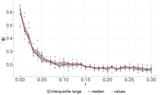
Figure 4.
Impact of the risk-free rate of return r on the average propensity to invest ().
SOs’ average propensity to invest directly influences the mean number of their frequency RBs leased on the secondary spectrum market (see Equation (1)). The hyperbolic shape of the relationship is depicted in Figure 5. Under the conditions we present in the model, the curve is identical with the one related to the risk-free rate of return and the average propensity to invest given in Figure 4. For a risk-free rate , the SO leases approximately 60 frequency RBs on average, whereas for , only 12 frequency RBs are leased. Given that the forward bid price is fixed, also the profit of the PO from the frequency spectrum lease given by Equation (7) depends solely on the volume of the frequency RBs leased to SOs in the forward market.
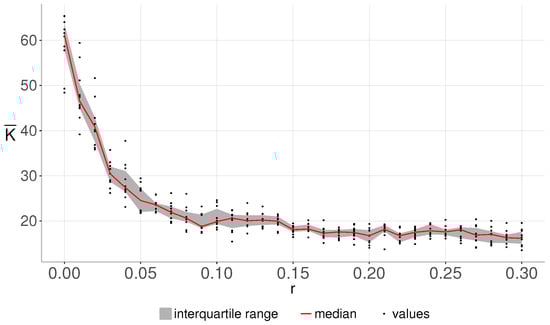
Figure 5.
Impact of the risk-free rate of return r on the number of RBs leased by an SO ().
SOs create the supply side of the retail market. Therefore, if the number of frequency RBs leased by SOs in the forward market decreases with an increase in the risk-free rate of return, then the supply in the retail market also decreases. For a fixed number of end users, the retail price must increase, resulting in retail price increases from risk-free rate increases, as presented in Figure 6.
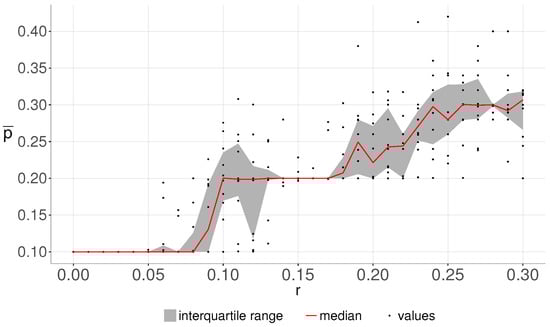
Figure 6.
Impact of risk-free rate of return r on average retail prices ().
The number of end user connections to the mobile network represents the level of end user satisfaction. A larger number of connections means that end user needs have been satisfied at a higher level and indicates higher availability of the frequency spectrum to end users, which depends on both the number of supplied frequency RBs in the retail market and the retail price. A higher retail price leads to lower availability of the frequency spectrum and vice versa. According to the analysis previously performed, if a higher risk-free rate of return results in fewer frequency RBs being leased by SOs in the forward market and higher retail connection prices, then it is evident that the higher risk-free rate causes a decrease in the number of connections. This is also confirmed in Figure 7.
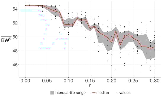
Figure 7.
Impact of risk-free rate of return r on average number of connections per SO ().
The main investment motive is to earn profits. In our model, two possibilities exist for the SO to gain profits. The SO receives a certain yield in the form of risk-free returns. A relationship exists between the risk-free rate of return r and the overall average daily return of the SO, as shown in Figure 8. If the risk-free rate of return equals 0, the SO’s overall daily profit is negligible because the SO can earn a profit only by investing in the frequency spectrum. Therefore, SOs that invest more than half of their budget in the frequency spectrum oversupply the retail market. This oversupply leads to low retail prices and low SO income. If the risk-free return is high, the SO invests almost all of its money risk-free; thus, its yield almost equals the invested amount. The linear relationship between the risk-free rate of return and the SO’s average daily return is given by the considerable financial resources invested risk-free. This relationship is also obvious from Figure 9, where the blue points represent the returns achieved on the secondary spectrum markets and the red points denote the risk-free returns. The long-term returns from the frequency spectrum are higher than those from the risk-free return, which is also one of the well-known laws in the theory of investments. The difference between the two returns is an extraordinary reward for the investor facing risks and is called the risk premium. The risk premium should be positive and long term, as proven in our simulation case. In contrast, the increase in the risk-free return also induces the increase in risky investments, as depicted in Figure 9.
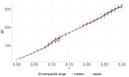
Figure 8.
Impact of risk-free rate of return r on average SO’s daily return ().
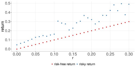
Figure 9.
Rate of returns on secondary spectrum market.
To this point, we have demonstrated the impact of risk-free rate of returns on various techno-economic indicators of the network. We have shown that the discovered relationships are not linear and the slopes of the relation curves in the figures vary according to the risk-free return level.
The market works under two distinct regimes.
- (1)
- Low risk-free rates of return .The retail market is saturated and extremely low prices prevail. The PO transfers the burden of a large number of the RBs to the SOs. The SOs are forced to lease the RBs on the secondary spectrum market even if they know that the retail market is oversupplied and they will achieve rather small profits. In contrast, even small changes in the risk-free returns trigger rather large changes in the number of forward trades and the economy of both the PO and the SOs. At the same time, the market remains saturated and low retail prices do not react to changes in risk-free returns.
- (2)
- High risk-free rates of return .The SOs are attracted to high risk-free returns and their forward trading activities decline. Low activity is also transferred to the retail market, where the supply remains insufficient and SOs sell their services for rather high prices. Their profits improve and both risk-free returns and retail trading profits increase. The positive increase in risk-free returns has a negligible impact on forward trading and the profits of the PO. In contrast, increasing retail prices reflect even smaller changes in risk-free returns. Trading volumes in the retail market change; end users reduce their outcomes; and demand becomes price sensitive.
7. Conclusions
In this paper, we analyzed the functioning of the open market with an internal organization similar to that proposed in Cramton and Doyle [11]. In this environment, we studied the impact of the financial risk-free rate of return on the secondary spectrum market. The designed market consists of both the forward market and the retail market. In the forward market, POs lease their unused spectra to SOs 360 days ahead in the form of forwards. SOs apply their forwards later in the retail market and sell the spectrum to end users who utilize the network services. The key element of the designed market is the existence of an open market that contains no barriers to entry for investors who do not need to operate their own network. Investors play the role of SOs whose only goal is to achieve their financial profits. The open market’s organization uses ideas from financial markets. Investors decide on the part of their budget to use for risk-free investments (out of the network) and the part that is invested in forwards.
Investors’ decisions are motivated by the risk-free rate of return transferred from the financial markets, but the return’s level regulates the techno-economic properties of the network as a whole. If the risk-free rate of return is high, SOs invest less in the secondary spectrum market and lease lower frequency RBs. Such an investment leads to lower supply in the retail market and retail prices increase, but it does not apply if the risk-free rate of return is low. Then, SOs are forced to lease a large amount of the forwards, causing an oversupply in the retail market. In this case, retail prices decline and utilization of the network increases.
This research has led to the discovery of some non-intuitive findings. First, if risk-free returns are small, retail trade prices and volumes are rather inelastic, and changes in the risk-free rate of returns do not influence the techno-economic properties of the network. The opposite is true for high risk-free returns. In this situation, the market is no more oversupplied and the price evolution and volume of retail trades reflect the evolution of the risk-free rate of return.
The simulated results show that they fully conform to the theory of the investments, i.e., risky returns resulting from investments in forwards are higher in the long term than the risk-free returns. In contrast, SOs’ profits increase when the risk-free rate of return increases.
To generalize these results, it is important to consider the fact that several limitations exist. We modeled a small local market with one PO, which affects the opportunity of SOs to invest their money. Obviously, in practice, the time frame (360 days) seems unrealistic; however, time rescaling is easy to apply in future research. The existence of other POs is also ignored; therefore, no competition exists between POs and SOs, and we assume a pure monopoly situation on the primary spectrum market. In terms of directions for further research, we aim to address this scenario with a more complex network topology.
Acknowledgments
This work was supported by the Slovak Research and Development Agency, project number APVV-15-0358.
Author Contributions
Juraj Gazda: research for the related works, doing the experiments, and drafting the paper. Peter Tóth and Marcel Vološin: Design of the complete model, the programming actions. Jana Zausinová and Vladimír Gazda: Total supervision of the paperwork, review, comments, assessment, and etc.
Conflicts of Interest
The authors declare no conflict of interest.
References
- Gantz, J.; Reinsel, D. Extracting value from chaos. IDC Iview 2011, 1142, 1–12. [Google Scholar]
- Whitacre, B.; Gallardo, R.; Strover, S. Broadband’s contribution to economic growth in rural areas: Moving towards a causal relationship. Telecommun. Policy 2014, 38, 1011–1023. [Google Scholar] [CrossRef]
- Jorgenson, D.W.; Vu, K.M. The ICT revolution, world economic growth, and policy issues. Telecommun. Policy 2016, 40, 383–397. [Google Scholar] [CrossRef]
- Wilson, A.; David, U.; Beatrice, E.; Mary, O. How telecommunication development aids economic growth: Evidence from ITU ICT development index (IDI) top five countries for African region. Int. J. Bus. Econ. Manag. 2014, 1, 16–28. [Google Scholar]
- Buddhikot, M.M. Understanding dynamic spectrum access: Models, taxonomy and challenges. In Proceedings of the 2nd IEEE International Symposium on New Frontiers in Dynamic Spectrum Access Networks, Dublin, Ireland, 17–20 April 2007; pp. 649–663. [Google Scholar]
- Hossain, E.; Niyato, D.; Han, Z. Dynamic Spectrum Access and Management in Cognitive Radio Networks; Cambridge University Press: Cambridge, UK, 2009. [Google Scholar]
- Peha, J.M. Approaches to spectrum sharing. IEEE Commun. Mag. 2005, 43, 10–12. [Google Scholar] [CrossRef]
- He, A.; Bae, K.K.; Newman, T.R.; Gaeddert, J.; Kim, K.; Menon, R.; Morales-Tirado, L.; Zhao, Y.; Reed, J.H.; Tranter, W.H.; et al. A survey of artificial intelligence for cognitive radios. IEEE Trans. Veh. Technol. 2010, 59, 1578–1592. [Google Scholar] [CrossRef]
- Evci, C.; Fino, B. Spectrum management, pricing, and efficiency control in broadband wireless communications. Proc. IEEE 2001, 89, 105–115. [Google Scholar] [CrossRef]
- Niyato, D.; Hossain, E. Spectrum trading in cognitive radio networks: A market-equilibrium-based approach. IEEE Wirel. Commun. 2008, 15, 71–80. [Google Scholar] [CrossRef]
- Cramton, P.; Doyle, L. Open access wireless markets. Telecommun. Policy 2017, 41, 379–390. [Google Scholar] [CrossRef]
- Malkiel, B.G.; Fama, E.F. Efficient capital markets: A review of theory and empirical work. J. Financ. 1970, 25, 383–417. [Google Scholar] [CrossRef]
- Fama, E.F. Efficient capital markets: II. J. Financ. 1991, 46, 1575–1617. [Google Scholar] [CrossRef]
- Markowitz, H. Portfolio selection. J. Financ. 1952, 7, 77–91. [Google Scholar]
- Tobin, J. Liquidity preference as behavior towards risk. Rev. Econ. Stud. 1958, 25, 65–86. [Google Scholar] [CrossRef]
- Li, Y.; Deng, H.; Peng, C.; Yuan, Z.; Tu, G.H.; Li, J.; Lu, S. iCellular: Device-Customized Cellular Network Access on Commodity Smartphones. In Proceedings of the 13th USENIX Symposium on Networked Systems Design and Implementation (NSDI), Santa Clara, CA, USA, 16–18 March 2016; pp. 643–656. [Google Scholar]
- Maier, M. Towards 5G: Decentralized routing in FiWi enhanced LTE-A HetNets. In Proceedings of the IEEE 16th International Conference on High Performance Switching and Routing (HPSR), Budapest, Hungary, 1–4 July 2015; pp. 1–6. [Google Scholar]
- Deng, H.; Li, Q.; Li, Y.; Lu, S.; Peng, C.; Raza, T.; Tan, Z.; Yuan, Z.; Zhang, Z. Towards Automated Intelligence in 5G Systems. In Proceedings of the 26th International Conference on Computer Communication and Networks (ICCCN), Vancouver, BC, Canada, 31 July–3 August 2017; pp. 1–9. [Google Scholar]
- Basaure, A.; Suomi, H.; Hämmäinen, H. Transaction vs. switching costs—Comparison of three core mechanisms for mobile markets. Telecommun. Policy 2016, 40, 545–566. [Google Scholar] [CrossRef]
- Shuminoski, T.; Janevski, T. 5G mobile terminals with advanced QoS-based user-centric aggregation (AQUA) for heterogeneous wireless and mobile networks. Wirel. Netw. 2016, 22, 1553–1570. [Google Scholar] [CrossRef]
- Hesmans, B.; Tran-Viet, H.; Sadre, R.; Bonaventure, O. A first look at real Multipath TCP traffic. In International Workshop on Traffic Monitoring and Analysis; Springer: Cham, Switzerland, 2015; pp. 233–246. [Google Scholar]
- Finley, B.; Basaure, A. Benefits of Mobile End User Network Switching and Multihoming. Computer Communications 2018, 117, 24–35. [Google Scholar] [CrossRef]
- De Carvalho, P.J.; Gupta, A.; Kar, K. Hierarchical spectrum market and the design of contracts for mobile providers. ACM SIGMOBILE Mob. Comput. Commun. Rev. 2013, 17, 60–71. [Google Scholar] [CrossRef]
- Gazda, J.; Kováč, V.; Tóth, P.; Drotár, P.; Gazda, V. Tax optimization in an agent-based model of real-time spectrum secondary market. Telecommun. Syst. 2017, 64, 543–558. [Google Scholar] [CrossRef]
- Gazda, J.; Bugár, G.; Vološin, M.; Drotár, P.; Horváth, D.; Gazda, V. Dynamic spectrum leasing and retail pricing using an experimental economy. Comput. Netw. 2017, 121, 173–184. [Google Scholar] [CrossRef]
- Veit, D.J.; Weidlich, A.; Yao, J.; Oren, S.S. Simulating the dynamics in two-settlement electricity markets via an agent-based approach. Int. J. Manag. Sci. Eng. Manag. 2006, 1, 83–97. [Google Scholar]
- Erev, I.; Roth, A.E. Predicting how people play games: Reinforcement learning in experimental games with unique, mixed strategy equilibria. Am. Econ. Rev. 1998, 88, 848–881. [Google Scholar]
- Tonmukayakul, A.; Weiss, M.B. A study of secondary spectrum use using agent-based computational economics. NETNOMICS Econ. Res. Electron. Netw. 2008, 9, 125–151. [Google Scholar] [CrossRef]
- Xing, Y.; Chandramouli, R.; Cordeiro, C. Price dynamics in competitive agile spectrum access markets. IEEE J. Sel. Areas Commun. 2007, 25, 613–621. [Google Scholar] [CrossRef]
- LeBaron, B. Agent-based computational finance. Handb. Comput. Econ. 2006, 2, 1187–1233. [Google Scholar]
- Ten Broeke, G.; Van Voorn, G.; Ligtenberg, A. Which sensitivity analysis method should I use for my agent-based model? J. Artif. Soc. Soc. Simul. 2016, 19. [Google Scholar] [CrossRef]
© 2017 by the authors. Licensee MDPI, Basel, Switzerland. This article is an open access article distributed under the terms and conditions of the Creative Commons Attribution (CC BY) license (http://creativecommons.org/licenses/by/4.0/).