Abstract
Recent developments in satellite data availability allow tropical forest monitoring to expand in two ways: (1) dense time series foster the development of new methods for mapping and monitoring dry tropical forests and (2) the combination of optical data and synthetic aperture radar (SAR) data reduces the problems resulting from frequent cloud cover and yields additional information. This paper covers both issues by analyzing the possibilities of using optical (Sentinel-2) and SAR (Sentinel-1) time series data for forest and land cover mapping for REDD+ (Reducing Emissions from Deforestation and Forest Degradation) applications in Malawi. The challenge is to combine these different data sources in order to make optimal use of their complementary information content. We compare the results of using different input data sets as well as of two methods for data combination. Results show that time-series of optical data lead to better results than mono-temporal optical data (+8% overall accuracy for forest mapping). Combination of optical and SAR data leads to further improvements: +5% in overall accuracy for land cover and +1.5% for forest mapping. With respect to the tested combination methods, the data-based combination performs slightly better (+1% overall accuracy) than the result-based Bayesian combination.
1. Introduction
Currently, operational forest monitoring in the dry tropics based on Earth Observation (EO) is limited by several issues: the phenology of tropical dry forest ecosystems with leaf fall in the dry season; frequent cloud cover during the rainy season and fast natural regrowth after deforestation or forest degradation events. The latter limits the time window within which forest changes can be detected. The use of time series of satellite data can help to overcome these limitations, especially when combining data from different but complementing sensors.
In this study, we test different methods for mapping forest and land cover classes at a dry forest site in Malawi. In the frame of the United Nations Framework Convention on Climate Change (UNFCCC) REDD+ (Reducing Emissions from Deforestation and Forest Degradation [1]), forest monitoring is not only defined by mapping forest and non-forest areas but also prescribes the classification of land cover (LC) classes defined by the Intergovernmental Panel on Climate Change (IPCC) and their changes over time in order to classify the deforested areas into these classes [2]. This is necessary to correctly budget the carbon losses, as different land cover classes have different carbon stocks. The IPCC land cover classes are: forest, grassland, agricultural land, wetland, settlement and other land.
Mapping and monitoring land cover changes and/or forests with strong phenology requires dense time series of EO data. With the launch of Sentinel-1A/B and Sentinel-2A/B a new era of frequent coverage of the earth surface by high resolution (HR) satellite imagery has started. Sentinel-1A was launched on 3 April 2014 and Sentinel-1B on 25 April 2016, both providing synthetic aperture radar (SAR) data in C-band at an azimuth resolution of approximately 20 m and a revisit time of six days at the equator. The optical sensors Sentinel-2A and Sentinel-2B were launched on 23 June 2015 and on 7 March 2017 respectively. They have a spectral resolution of 13 bands in the optical to infrared wavelengths. The ground resolution is—depending on the spectral bands–10, 20 or 60 m. The revisit time is five days at the equator. In conjunction with the Landsat mission satellites, Sentinel data stacks allow for improved land cover mapping by analyzing seasonal changes of vegetation cover. The volume of data generated by Sentinel and other satellite systems requires sophisticated methods and algorithms to compute wall-to-wall maps that are based on dense time series data stacks. Efficient methods are needed for time series analysis and to integrate SAR and optical data in operational processing chains for forest and land use mapping
Mapping approaches based on Sentinel-1 SAR (time series) data have been proposed for classifying urban areas [3], general land cover classes [4,5]; forests [6,7,8,9,10]; water bodies or flooding [11,12,13] and croplands/grasslands [14,15]. Also, some recent studies on tropical forest monitoring are based on L-band data (e.g., [16,17]). Due to the large amount of papers using Sentinel-2 for different land cover applications, only a limited number of selected land cover classifications can be listed here, which include: vegetation mapping [18,19], agricultural applications [20,21], water related applications [22] and forest mapping [23,24,25,26,27]. Pre-processing is a crucial part of the whole processing chain as errors or missing steps greatly influence the quality of intermediate and final results. The pre-processing of images for a time series is even more demanding than for single image classification or bi-temporal change detection, as many images need to be geometrically and radiometrically consistent to extract the required information [28].
With respect to data combination, the reader is kindly referred to a review article on optical and radar remote sensing data combination for land cover and land use mapping and monitoring [29] which covers most relevant literature in the field until the end of 2015. In this review [29], 37 out of 50 studies are described to perform a data-based combination, partly in a traditional sense of some kind of “pan-sharpening” approach followed by traditional image classification, partly using machine learning or decision tree algorithms. The Random Forest (RF) classifier has been used frequently, as it has proven to be well capable of forest and land cover mapping and can handle large amounts of data, also from different sources [30,31,32]. RF belongs to the ensemble learning methods together with other boosting and bagging methods and classification trees. These classifiers generate many classifiers and aggregate their results to calculate the final response [32,33,34]. RF methods can be used for multi-source data classification and have been successfully used for classification of different tree types [35]. The RF algorithm learns the relationship between predictor and response data and can handle continuous, categorical and binary data sets [30,31,32]. It offers a good prediction performance and is computationally effective. RF is therefore well suitable to analyze different sets of input data, while keeping all other parameters constant.
In recent studies, SAR data has only been used for stratification purposes [36], while classification of the target class was based on optical data alone. Similarly, a step-wise approach for combination was applied for mangrove mapping [37]. They use S1 time series to generate a standing water map, which is then used as input together with classes derived from optical data in a decision tree algorithm to classify mangrove forest. Some studies focus on comparing time series of Sentinel-1 features with Sentinel-2 or other optical data features [38] and conclude with a recommendation to jointly use both data sources. Data-based combination methods are also used for biomass estimation, for which a multi-variate regression model is built on both input data sets [39]. Bayesian combination is a result-based combination method and is mainly used for forest disturbance mapping with optical and SAR data [23,40,41]. Another method of result-based combination is just simply adding independently generated detections from both sensors [42]. Although there is a large amount of literature on land cover classification, there are very few studies using both optical and SAR time-series data for land cover classification [43,44,45,46]. Although most studies on data combination demonstrate improvements in land cover classification by combining different sensor data there is still a lack of proper validation methods and of combination methods for time series of data [29]. Currently, the resulting research needs can be summarized as follows: (1) demonstrating applicability for large areas and not only for small test sites; (2) developing robust optical and radar data combination techniques for time series of data and datasets of different spatial resolution; and (3) validating results based on a set of permanent ground-based measurements [29]. To our knowledge, these research needs are not fully addressed yet. In our study, we address two of these needs by quantitatively assessing the improvement of using time-series as input data and of using different data combination methods for large area operational mapping purposes. To do so, we test two different combination methods: first, a data-based combination and second, a result-based Bayesian combination.
In conclusion, in this paper, we tackle three research questions:
- (1)
- What is the added value of using time series data versus mono-temporal remote sensing data?
- (2)
- What is the added value of combining optical and SAR time series data?
- (3)
- Which of the two tested combination approaches (data-based vs. result-based) performs better?
2. Study Area and Data
The study area is located in the central-northern part of Malawi, around the city of Mzimba and covers an area of 4500 km2 (Figure 1). In the study area, all five IPCC land cover classes are available with a main share of forest (about 62%); further 29% cropland, 6% grassland and the rest settlements and wetlands. The forest definition we use in this study is in line with the FAO (Food and Agriculture Organization of the United Nations) definition: potential tree height at maturity is 5 m, minimum tree crown cover is 10% and the minimum mapping unit is 0.5 ha.
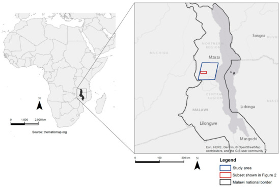
Figure 1.
Location of study area and subset depicted in Figure 2.
The study area is very heterogeneous: while the eastern areas, close to Lake Malawi, still receive significant rainfall, the western part of the study area is very dry. The area is thus characterized by a spatial phenology gradient from medium to strong phenology from east to west. Consequently, the forested areas differ strongly in tree cover density and tree type composition and therefore show very different spectral behavior. Dry forests and the surrounding land use classes are more difficult to classify than humid evergreen forests, as they show typical phenological development from highly vital in the rainy season to dry and leafless in the dry season. It is therefore already challenging to generate and update a forest change mask for the study area, as observed spectral changes in the forest are not only resulting from forest area change but also from differences in the phenological stage of the forests. Other factors such as burning bushes beneath the canopy can further complicate forest classification.
The mapping challenges in the study area are thus the gradual spatial change from east to west and the temporal difference in phenology from year to year. For example, one year, the rainy season might start by the beginning of November; the next year it starts in December. Precipitation data, which is available for Mzuzu, located 25 km north of the study area, shows this effect (see Table 1, from www.weatheronline.co.uk). This situation clearly affects and significantly complicates forest and land cover classification.

Table 1.
Monthly precipitation for Mzuzu (Malawi) in different years.
We performed a visual pre-analysis to assess the phenological behavior on the time series image stack. Figure 2 shows a forest area (subset in Figure 1) in different stages between December 2015 and December 2016. All images are atmospherically corrected to “Bottom-of-Atmosphere” (BoA) values and displayed with the same LUT (look-up table) stretch in the following red/green/blue (RGB) bands: R = short wave infrared (SWIR), G = near infrared (NIR), B = red. Thus, the differences in the images entirely stem from phenology and vegetation changes. The areas affected by below-canopy fires appear in red-brown from September to November. Standard change detection procedures would detect deforestation between December 2015 and November 2016. However, after the start of the next rainy season, the situation appears almost unchanged in December 2016 compared to December 2015. Therefore, either the use of data from exactly the same phenological stage or the use of time series data is required to avoid misclassifications and to reach the needed accuracy level. Determining the date with the exact same phenological stage is very difficult due to the inter-annual variations outlined above and the varying cloud cover. In addition to phenological effects, short term effects are also influencing classification results: haze, smoke, clouds and cloud shadows in optical images for example. SAR data is not affected by clouds, haze or smoke but reacts sensitive to moisture. Therefore, a single SAR image after a rainfall would give a much different result than during a dry period. In conclusion, the pre-analysis showed that using time series data is currently the most promising approach for classifying dry forests.
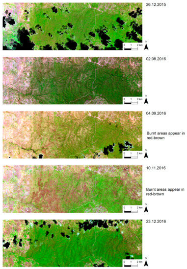
Figure 2.
Visualization of extreme phenology in combination with sub-canopy fires in the Miombo forest in Malawi mapped with Sentinel-2. All images with same LUT stretch (R = SWIR, G = NIR, B = Red) Subset of the study area, location of this subset is shown in Figure 1.
We employed altogether 15 Sentinel-2 scenes acquired between 26 December 2015 and 18 February 2017. For Sentinel-1, we used 14 Ground Range Detected (GRD) high resolution ascending scenes between 28 April 2016 and 23 April 2017. All acquisition dates and the main properties of the used data sets are listed in Table 2.
Table 2.
Input data and data properties.
3. Methods
3.1. Pre-Processing Methods
For the optical data stacks, we applied the following pre-processing steps: (1) atmospheric correction, (2) cloud masking and (3) topographic correction. For atmospheric correction of Sentinel-2 data to bottom-of-atmosphere reflection we use the open-source software Sen2Cor Version 2.3.1 [47]. The Sen2Cor scene classification results are used to derive a preliminary cloud mask [48]. Based on this preliminary mask, the following post-processing steps are applied to further improve the quality of the cloud masks: morphological operations on the initial mask to remove road pixels wrongly classified as clouds; morphological closing to generate more compact cloud areas and finally removal of valid areas within and near detected cloud areas, as they are often affected by neighboring clouds. Topographic correction was performed with the self-calibrating topographic normalization tool [49]. These pre-processed images were used for all further work in this study.
The Sentinel-1 GRD high resolution SAR data was pre-processed with Joanneum Research RSG software Version 7.51.0 (www.remotesensing.at, [8]). First, we ingested the images and updated the orbit parameters. Then, we processed the images to gamma naught based on the SRTM (Shuttle Radar Topography Mission) digital elevation model. Next, we applied a multi-looking of 2 by 2 ground range looks to 20m final pixel spacing. Multi-looking can be seen as a kind of mean filter in radar data processing. We registered each image to a master image (first image of the stack) to avoid geometrical inconsistencies. For noise reduction, we employed a Quegan multi-temporal filter with a 3 × 3 spatial window [50]. Multi-temporal speckle filtered SAR images usually show higher performance in terms of noise reduction and preservation of spatial information than single speckle-filtered SAR images or unfiltered SAR images [51]. The stack of time series data was then analyzed by statistical methods resulting in the following statistics stack: mean, minimum and maximum backscatter, standard deviation, coefficient of variation, trend between first three and last three images. The registered stack of statistics images was then ortho-rectified to 20 m spatial resolution for further use. The main reasons for using this stack as opposed to the individual images are twofold: first, the “mean” image shows much lower speckle than the individual images, which improves classification accuracy. Second, different land cover classes show specific behavior over the year, which are well represented by “standard deviation” and “coefficient of variation” of the stack.
3.2. Classification Methods for Mono-Temporal and Time-Series Data
In order to answer the first research question, that is, to compare mono-temporal and time series based results of optical data, we selected different feature sets and employed the Random Forest (RF) classifier of the Orfeo Toolbox (OTB, [52]). order to obtain reliable training data, we visually interpreted and delineated representative areas for all land cover classes from VHR images. We then used these areas as training data set for the RF classifier.
For SAR, we did not perform a comparison of mono-temporal and time series data. According to various studies [50,53], it is generally accepted that classifications based on a mono-temporal SAR image are performing worse than those based on time-series of SAR data. Multi-temporal speckle filters that are frequently applied to SAR time series can considerably increase the signal-to-noise ratio of SAR images [50,53]. Therefore, we only analyze time series of SAR data in this study.
3.3. Methods for Combined Use of Optical and SAR Time Series Data
We employed and compared two different methods for the combination of optical and SAR data: first, a data-based combination, where all pre-processed data were included in the same RF classification step. Pre-processed data comprises the bands of Sentinel-2 on the one hand and the statistics stack of Sentinel-1 on the other hand (see Table 1 and Section 3.1).
Second, we employed a result-based combination using the Bayesian principle. For the result-based combination, the probability (or likelihood) of a pixel belonging to a certain class (e.g., forest or deforestation) is generated from the optical and SAR processing chain separately and independently [54,55] using so-called probability density functions (pdfs) or probability functions (pf) depending on the generation method. The pdfs/pfs are generated separately for each data type (optical or SAR) using the same set of training data for the required classes. These training areas were selected specifically for the training purpose and are the same as explained in Section 3.2. In addition to the probability, also a reliability measure for both data types can be applied. If no reliability measure is available, both data types can be considered equally reliable. In reality, the reliabilities can be very different and even spatially heterogeneous; for example in mountainous areas, SAR reliability should be lower due to layover and foreshortening effects [56,57]. One way to estimate the reliability of the individual results is by independent accuracy assessment using validation samples as explained in Section 3.4. The individual results from SAR and optical data are then merged using a system based on Bayes’ theorem. The whole Bayesian combination workflow is shown in Figure 3 below.
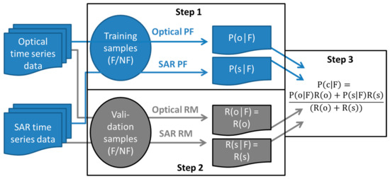
Figure 3.
Schematic workflow of the Bayesian combination method.
The first step is to generate conditional probabilities for each pixel and separately for each data type. P(o│F) is the probability of a pixel to be forest based on optical data and P(s│F) is the probability of a pixel to be forest based on SAR data. For this calculation, we use probability functions (PF) implemented in the RF classifier in Python. The probability is defined as the mean predicted class probabilities of the decision trees in the RF classifier. The class probability of a single decision tree is the fraction of samples of the same class in a leaf. This means, if one pixel is classified 8 of 10 “leaves” as forest, the probability is 0.8. Some considerations and detailed discussions about the calculation of probabilities from RF classifiers can be found in Reference [58].
The second step is the reliability measurement (RM) for each data type, R(o│F) and R(s│F) respectively. R(o│F) is the reliability of a pixel to be forest based on optical data and R(s│F) is the reliability of a pixel to be forest based on SAR data. For the calculation, we used an independent accuracy analysis using a set of validation samples (see Section 3.4). In our study, we did not use the class specific reliabilities but the overall accuracy (integrating all classes) as a general measure of reliability. Thus, the reliability of forest R(o│F) would be equal to the reliability of non-forest R(o│NF) and we can denote R(o) = R(o│F) and R(s) = R(s│F) for simplicity.
The third step is to combine both probabilities by considering the reliabilities according to the following equation, where P(c│F) is the combined probability for a pixel to belong to the class forest:
3.4. Validation Method
For accuracy assessment and for the estimation of the reliability for each data type, we visually interpreted a regular grid of 1918 plots in Google Earth (GE). The advantage of systematic sampling is that “it maximizes the average distance between plots and therefore minimizes spatial correlation among observations and increases statistical efficiency” [59]. Stratified random sampling is necessary, if for example field work efforts or data availability does not allow a full coverage. Since very high resolution (VHR) imagery in GE is available for most of the prototype site and often for several dates, such restrictions do not apply. The VHR imagery used within GE is provided by different sensors such as Pléiades, GeoEye or WorldView. The data has a spatial resolution of 1 m or better. Only the visible bands are available for interpretation. Using the time function, we used only images of 2015 ± one year for the validation. Of the total 1918 plots, 439 plots could not be interpreted for forest/non-forest leaving 1479 valid plots. There are three reasons for this: (1) a lack of recent VHR data (for reference year 2016), (2) points could not be interpreted reliably due to clouds, shadows or land use in transition phase, (3) some plots are located at the fringe of forest and due to geometric inaccuracies between GE and the input data, these points cannot be considered as reliable and therefore are excluded from the validation data set. For LC, 119 additional plots were rejected due to their location at non-forest class borders. This left 1360 valid plots for the LC map validation.
The valid plots were used for an extensive accuracy assessment of the forest/non-forest (FNF) maps and the LC classifications. The interpretation was done fully blind and the results were used for comparing the different data sets and the two combination methods (data-based and result-based combination). The results are presented in Table 3 and Table 4. Before evaluating the final map, we performed an additional plausibility check for plots that were considered wrongly classified. This step was necessary, as in Malawi, pixels can be attributed to different LC classes within one year (e.g., flooded/wetland in rainy season, cropland in dry season).
Table 3.
Accuracies of mono-temporal versus time series approach for FNF maps.
Table 4.
Accuracies of mono-temporal versus time series approach for IPCC LC classes.
We used two different methods for accuracy assessment: (1) in count-based assessment, each plot has the same weight, independent from the frequency of the assigned class; (2) in area-based assessment, each plot represents a certain area according to the frequency of the different classes the plots have been assigned to. Thus, a plot representing a frequent class gets a higher weight in the accuracy assessment than a plot with a class of rare occurrence [60,61,62]. The latter approach is needed in order to calculate confidence intervals (CI) per class, which are important in the carbon reporting for IPCC. In our study, we used the count-based approach for all method and data comparisons and the area-based approach for the final maps only.
4. Results
4.1. Forest/Non-Forest Mapping and LC Classification: Optical Mono-Temporal Versus Optical Time Series Results
For the optical mono-temporal classification approach the best scene in terms of cloud cover and phenological stage was selected, that is: least cloud cover and leaf-on season. For the optical time series analysis approach, different optical input data set combinations were tested in the RF classifier using the same training samples. The selection was done based on image data quality, cloud cover and temporal distribution. The target year for classification was 2016. The input data sets for the optical classification approaches are:
- Mono-temporal: Sentinel-2 image from 02.08.2016 (very good quality image, see Figure 2)
- Time series variant 1 (V1): 23.07.2016, 02.08.2016, 12.08.2016
- Time series variant 2 (V2): 26.12.2015, 02.08.2016, 12.08.2016, 10.11.2016
- Time series variant 3 (V3): 26.12.2015, 14.05.2016, 23.07.2016, 10.11.2016
- Time series variant 4 (V4): 26.12.2015, 14.05.2016, 23.07.2016, 02.08.2016, 12.08.2016, 10.11.2016
- Time series all: All optical images available for 2016 including those with low quality or high cloud cover.
The reason for selecting different subsets is to see, whether some images from “key dates” have the same information content as all images. Due to positive and negative correlations between images, the option using all images cannot necessarily be expected to be the best option. The accuracies of the optical data sets are given in Table 3. The advantage of using multi-temporal data versus mono-temporal data even for a status product such as forest/non-forest is obvious.
4.2. Combination of SAR and Optical Time-Series Data Sets for FNF Maps
As regards SAR data, the focus of this study was on combining SAR data with optical data. Previous studies [63,64] have found cross-polarized images (VH) to be better suited for forest monitoring which is why we limited our analysis to cross-polarized data in this study. For the SAR time series data classification, the SAR data was processed to a statistic stack as explained in Section 3.1. The combination of optical and SAR data was done according to the methods’ descriptions given in Section 3 of this paper. For the data-based combination, the SAR statistics stack was included in the RF classifier together with the optical data. For the result-based combination, this stack was separately classified using RF. The reliability used in the Bayesian combination is the OA for the individual results given in Table 4 under “Optical only” and “SAR only.” For example, the reliability for the optical mono-temporal result is 0.759. For all classifications—regardless of the input data—the same training samples were used to train the classifier. The FNF mapping accuracies based on the validation plots are shown in Table 5. We achieved the best result by combining optical V4 time series and SAR time series data with the data-based combination approach (blind OA 0.8526) followed by the result-based combination of the same data sets (OA 0.8425 in Table 5). For a comparative overview, we repeat the values for optical data only (same as in Table 3). We found out that the use of optical time series data leads to almost the same results in OA (0.8364) as the use of mono-temporal optical data in combination with SAR time series data (0.8319).
Table 5.
Accuracies of optical/SAR only and optical/SAR combined approaches for FNF maps.
A visual comparison of the generated forest maps is shown in Figure 4. For better visibility of the detailed differences, a subset of the whole study area is depicted. All quantitative assessments are based on the whole study area.
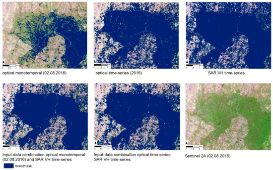
Figure 4.
Visualization of forest maps from different input data sets and data-based combination for a subset in Malawi.
The best map (time-series V4 & SAR VH, data-based combination) was re-validated with an area-based validation approach using the same validation points after a plausibility analysis and by calculating and applying area-specific weights as described in Section 3 [60,61,62]. The area-specific weights are generated based on the map and are 0.55 for forest and 0.45 for non-forest (see Section 3.3). The resulting map (Figure 5) has an area-based overall accuracy of 94%; Table 6 shows all details including users’ and producers’ accuracies and confidence intervals (CI).
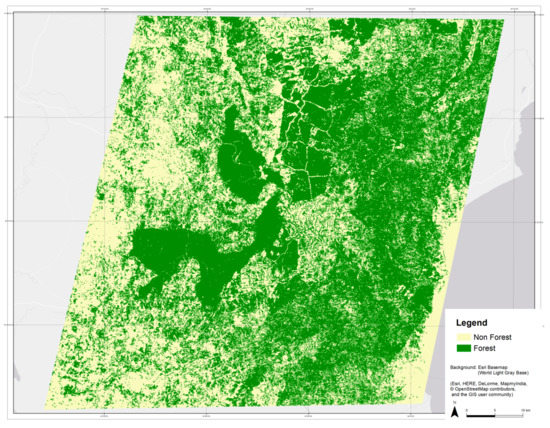
Figure 5.
Final FNF map based on combined optical and SAR time series data.
Table 6.
Confusion matrix of the final FNF map of Malawi after plausibility check.
4.3. Combination of SAR and Optical Time-Series Data Sets for LC Maps
Due to the fact that data-based SAR /optical combination performed better for FNF, we also applied the data-based combination to map IPCC land cover classes. The OA results are given in Table 7. Again, we repeat the values for optical data only in order to provide easier comparison. We validated the final map in the same manner (area-based and plausibility checked) as the best FNF map, which results in an OA of 85.04% and a CI of 80.90–90.18%.
Table 7.
Accuracies of optical only and optical/SAR combined approach for IPCC LC classes.
4.4. Comparison with Existing Products
We compared our results also with two existing mapping products: (1) the Global Forest Watch (GFW) FNF map of the year 2000 updated with gains and losses between 2000 and 2016 (available at: https://www.globalforestwatch.org/map); and (2) the CCI land cover map of Africa for 2016 (available at: http://2016africalandcover20m.esrin.esa.int/). The GFW FNF map is a global map of forest areas based on Landsat data with 30 m spatial resolution. The CCI map is a prototype of a high-resolution LC map at 20m spatial resolution over Africa based on one year of Sentinel-2A observations from December 2015 to December 2016. The improvement of our best time series result based on optical data only compared to the existing products is more than 12%. When comparing our overall best result, we achieve an improvement of almost 14% (see Table 8). For IPCC LC classes, we compared our best result to the CCI map only, as GFW does not provide LC information. The OA accuracy of CCI Land Cover is 0.6507 (kappa = 0.43) compared to our best result with an OA of 0.7870 (kappa = 0.6); see Table 6.
Table 8.
FNF accuracy compared to existing products.
5. Discussion
The benefits of using both optical and SAR data for forest and LC mapping depend strongly on the specific site characteristics and the output product specifications. For dry forests with a medium to strong phenology, time series data is especially important. An alternative approach to using all images in classification is the use of a multi-temporal filter as a pre-processing step [65]. With respect to our first research question, we can state that the added value of using time series data versus mono-temporal optical remote sensing data for forest and LC mapping in our study area in the dry tropics is significant. The improvement in overall accuracies (OA) is—depending on the used time series data set—between 3.5% and almost 8%. Another benefit of using times series as input is that no-data areas due to cloud and cloud shadows can be avoided. The best result was achieved using all “good” images of the time series (V4). When integrating more data, that is, all available images, the results deteriorate. The reason can be found in the low quality of some scenes, which are affected by haze, smoke or their quality suffers from inaccurate cloud masking. For the LC classification (Table 4) only the worst (V1) and the best (V4) time-series variants of FNF mapping were used to highlight the range of potential improvement, which is between +4 and +6%.
Regarding the added value of combining optical and SAR time series data (research question 2), the improvement is not as significant as for mono-temporal versus time-series data. The quantitative improvement is 1.5% in OA for FNF. This finding is in line with various recent publications [66,67,68,69,70]. For LC, the combined use of optical and SAR data also improved the overall accuracy compared to using one data type only. We achieved the best result by combining mono-temporal optical data with SAR time-series followed by time-series optical with SAR time-series. The added value is almost 5% in OA for LC. Similar results have been presented previously, although partly based on other input data sets such as ALOS PALSAR combined with Landsat [70,71,72,73,74]. As regards SAR data, the focus of this study was on combining SAR data with optical data. Previous studies [63,64] have found cross-polarized images to be better suited for forest monitoring which is why we limited our analysis on cross-polarized data in this study. Since recent research studies have achieved better results with co-polarized Sentinel-1 data [42] future research should also analyze the integration of different SAR polarizations and polarimetric features for the combined approach.
With respect to combination methods for optical and SAR data, we found that the data-based combination led to slightly better results than the result-based combination for FNF mapping. However, other studies showed good results with result-based Bayesian combination for forest disturbance mapping [23,41,55,75]. A difference between our approach and the one used in the literature [55] is the method to generate the probability values. While we used the probabilities derived from the RF classification (see Section 3.2) [55] employs a probability density function (pdf) using a Maximum Likelihood classifier. The pdf requires a Gaussian distribution of the training samples to derive useful results. A comparison of the two approaches to generate the probability values on the same data sets and study area would allow better understanding of these dependencies.
We also compared our results with existing products from global and regional mapping initiatives. The global product (GFW) is based on Landsat data and updated with losses and gains, which are published regularly as a new image becomes available. The CCI products are based on Sentinel-2 data from December 2015 to December 2016 and classified with RF and machine learning separately and then combined. Thus, from the input data used for the classification, the CCI map is comparable to our optical time series results, while for the GFW, the input data is different and of lower spatial resolution. It can be expected, that global or regional products are outperformed by approaches with a local focus and related local reference data. The aim of this comparison is to provide potential users, such as national entities in charge of IPCC reporting, a quantitative comparison of these differences and to demonstrate the improvements that are possible with a locally focused analysis. Finally, our results strongly support a systematic inclusion of SAR data in REDD+ mapping efforts.
6. Conclusions
This study focuses on REDD+ monitoring in dry tropical forests in Malawi. We investigated the performance of optical and SAR data and their combination for forest and land cover mapping in this area. First, it was investigated, if time-series of optical data leads to better results than using mono-temporal data. Second, we quantitatively assessed the added value of integrating SAR time series data in addition to the optical data. Third, we tested two options for the combined use of optical and SAR time series data and compared their performance.
We achieved an increase in OA for forest mapping of 8% and an increase for land cover mapping of 6%, when using optical time series data instead of single image use. In addition, this approach also reduced the amount of no-data values in the final products. The results further show a clear improvement of using a combination of SAR (Sentinel-1) and optical data (Sentinel-2) compared to only using data from one data type. Combination of optical and SAR data leads to improvements of 5% in overall accuracy for land cover and 1.5% for forest mapping compared to using optical time series data only. With respect to the tested combination methods, the data-based combination performs slightly better (+1% OA) than the result-based combination. Mono-temporal optical data in combination with SAR time series led to similar accuracies as optical time-series data alone. Thus, SAR time-series data can potentially replace optical time-series data sets, if those are affected by clouds and/or haze or smoke.
The use of common validation data for comparing different approaches remains a research need already posed [29]. However, such an exercise is only useful, if this common validation data is not used for training purposes. Otherwise, the validation would not be independent and thus would lead to biased results. In terms of combination methods, future research should include the comparison of different methods to estimate the probabilities in the classification step. Another important research gap is to test the transferability of proposed methods to other and even larger areas. Finally, with regard to REDD+ monitoring requirements, the mapping of forest degradation in dry forest areas remains a huge challenge and might require new sophisticated tools for phenology modelling to efficiently differentiate between forest degradation and phenological change effects.
Author Contributions
Conceptualization, M.H.; Data curation, C.S.; Formal analysis, C.S.; Investigation, M.H. and C.S.; Methodology, M.H., J.D. and M.S.; Project administration, M.H.; Validation, M.H.; Writing—original draft, M.H.; Writing—review & editing, J.D. and M.S.
Funding
This project has received funding from the European Union’s Horizon 2020 research and innovation program under grant agreement No 685761 (EOMonDIS) including the funds for open access.
Acknowledgments
The authors would like to thank the anonymous reviewers for their valuable comments, which greatly helped to improve this paper.
Conflicts of Interest
The authors declare no conflict of interest.
References
- Parker, N.C.; Mitchell, A.; Trivedi, M. The Little REDD+ Book: An Updated Guide to Governmental and Non-Governmental Proposals for Reducing Emissions from Deforestation and Degradation, 2nd ed.; Global Canopy Foundation: Oxford, UK, 2009; p. 132. [Google Scholar]
- IPCC Good Practice Guidance for Land Use, Land-Use Change and Forestry (GPG-LULUCF). 2003. Available online: http://www.ipcc-nggip.iges.or.jp/public/gpglulucf/gpglulucf_contents.html (accessed on 8 October 2018).
- Pesaresi, M.; Corbane, C.; Julea, A.; Florczyk, A.; Syrris, V.; Soille, P. Assessment of the Added-Value of Sentinel-2 for Detecting Built-up Areas. Remote Sens. 2016, 8, 299. [Google Scholar] [CrossRef]
- Abdikan, S.; Sanli, F.B.; Ustuner, M.; Calò, F. Land Cover Mapping using Sentinel-1 SAR Data. Int. Archives Photogramm. Remote Sens. 2016, 41, 757–761. [Google Scholar] [CrossRef]
- Balzter, H.; Cole, B.; Thiel, C.; Schmullius, C. Mapping CORINE land cover from Sentinel-1A SAR and SRTM digital elevation model data using Random Forests. Remote Sens. 2015, 7, 14876–14898. [Google Scholar] [CrossRef]
- Antropov, O.; Rauste, Y.; Väänänen, A.; Mutanen, T.; Häme, T. Mapping forest disturbance using long time series of Sentinel-1 data: Case studies over boreal and tropical forests. In Proceedings of the 2016 IEEE International Geoscience and Remote Sensing Symposium (IGARSS), Beijing, China, 10–12 July 2016; pp. 3906–3909. [Google Scholar] [CrossRef]
- Delgado-Aguilar, M.J.; Fassnacht, F.E.; Peralvo, M.; Gross, C.P.; Schmitt, C.B. Potential of TerraSAR-X and Sentinel 1 imagery to map deforested areas and derive degradation status in complex rain forests of Ecuador. Int. For. Rev. 2017, 19, 102–118. [Google Scholar] [CrossRef]
- Deutscher, J.; Gutjahr, K.; Perko, R.; Raggam, H.; Hirschmugl, M.; Schardt, M. Humid tropical forest monitoring with multi-temporal L-, C- and X-Band SAR data. In Proceedings of the 2017 9th International Workshop on the Analysis of Multitemporal Remote Sensing Images (MultiTemp), Bruges, Belgium, 27–29 June 2017. [Google Scholar]
- Dostálová, A.; Hollaus, M.; Milutin, I.; Wagner, W. Forest Area Derivation from Sentinel-1 Data. ISPRS Ann. Photogram. Remote Sens. Spat. Inf. Sci. 2016, 3, 227–233. [Google Scholar] [CrossRef]
- Haarpaintner, J.; Davids, C.; Storvold, R.; Johansen, K.; Ãrnason, K.; Rauste, Y.; Mutanen, T. Boreal Forest Land Cover Mapping in Iceland and Finland Using Sentinel-1A. In Proceedings of the Living Planet Symposium 2016, Prague, Czech Republic, 9–13 May 2016; Volume 740, p. 197, ISBN 978-92-9221-305-3. [Google Scholar]
- Pham-Duc, B.; Prigent, C.; Aires, F. Surface Water Monitoring within Cambodia and the Vietnamese Mekong Delta over a Year, with Sentinel-1 SAR Observations. Water 2017, 9, 366. [Google Scholar] [CrossRef]
- Plank, S.; Jüssi, M.; Martinis, S.; Twele, A. Mapping of flooded vegetation by means of polarimetric Sentinel-1 and ALOS-2/PALSAR-2 imagery. Int. J. Remote Sens. 2017, 38, 3831–3850. [Google Scholar] [CrossRef]
- Twele, A.; Cao, W.; Plank, S.; Martinis, S. Sentinel-1-based flood mapping: a fully automated processing chain. Int. J. Remote Sens. 2016, 37, 2990–3004. [Google Scholar] [CrossRef]
- Nguyen, D.B.; Wagner, W. European Rice Cropland Mapping with Sentinel-1 Data: The Mediterranean Region Case Study. Water 2017, 9, 392. [Google Scholar] [CrossRef]
- Tamm, T.; Zalite, K.; Voormansik, K.; Talgre, L. Relating Sentinel-1 Interferometric Coherence to Mowing Events on Grasslands. Remote Sens. 2016, 8, 802. [Google Scholar] [CrossRef]
- Mermoz, S.; Le Toan, T. Forest Disturbances and Regrowth Assessment Using ALOS PALSAR Data from 2007 to 2010 in Vietnam, Cambodia and Lao PDR. Remote Sens. 2016, 8, 217. [Google Scholar] [CrossRef]
- Mermoz, S.; Réjou-Méchain, M.; Villard, L.; Toan, T.L.; Rossi, V.; Gourlet-Fleury, S. Decrease of L-band SAR backscatter with biomass of dense forests. Remote Sens. Environ. 2015, 159, 307–317. [Google Scholar] [CrossRef]
- Sharma, R.C.; Hara, K.; Tateishi, R. High-Resolution Vegetation Mapping in Japan by Combining Sentinel-2 and Landsat 8 Based Multi-Temporal Datasets through Machine Learning and Cross-Validation Approach. Land 2017, 6, 50. [Google Scholar] [CrossRef]
- Shoko, C.; Mutanga, O. Examining the strength of the newly-launched Sentinel 2 MSI sensor in detecting and discriminating subtle differences between C3 and C4 grass species. ISPRS J. Photogram. Remote Sens. 2017, 129, 32–40. [Google Scholar] [CrossRef]
- Solano-Correa, Y.T.; Bovolo, F.; Bruzzone, L.; Fernández-Prieto, D. Spatio-temporal evolution of crop fields in Sentinel-2 Satellite Image Time Series. In Proceedings of the 2017 9th International Workshop on the Analysis of Multitemporal Remote Sensing Images (MultiTemp), Bruges, Belgium, 7–29 June 2017. [Google Scholar]
- Zhang, T.; Su, J.; Liu, C.; Chen, W.-H.; Liu, H.; Liu, G. Band Selection in Sentinel-2 Satellite for Agriculture Applications. In Proceedings of the 2017 23rd International Conference on Automation & Computing, Huddersfield, UK, 7–8 September 2017. [Google Scholar]
- Toming, K.; Kutser, T.; Laas, A.; Sepp, M.; Paavel, B.; Nges, T. First experiences in mapping lake water quality parameters with Sentinel-2 MSI imagery. Remote Sens. 2016, 8, 640. [Google Scholar] [CrossRef]
- Hirschmugl, M.; Deutscher, J.; Gutjahr, K.-H.; Sobe, C.; Schardt, M. Combined Use of SAR and Optical Time Series Data for Near Real-Time Forest Disturbance Mapping. In Proceedings of the 2017 9th International Workshop on the Analysis of Multitemporal Remote Sensing Images (MultiTemp), Bruges, Belgium, 7–29 June 2017. [Google Scholar]
- Immitzer, M.; Vuolo, F.; Atzberger, C. First Experience with Sentinel-2 Data for Crop and Tree Species Classifications in Central Europe. Remote Sens. 2016, 8, 166. [Google Scholar] [CrossRef]
- Majasalmi, T.; Rautiainen, M. The potential of Sentinel-2 data for estimating biophysical variables in a boreal forest: A simulation study. Remote Sens. Lett. 2016, 7, 427–436. [Google Scholar] [CrossRef]
- Simonetti, D.; Marelli, A.; Rodriguez, D.; Vasilev, V.; Strobl, P.; Burger, A.; Soille, P.; Achard, F.; Eva, H.; Stibig, H.; et al. Sentinel-2 Web Platform for REDD+ Monitoring. 2017. Available online: https://www.researchgate.net/publication/317781159 (accessed on 9 October 2018).
- Sothe, C.; de Almeida, C.M.; Liesenberg, V.; Schimalski, M.B. Evaluating Sentinel-2 and Landsat-8 Data to Map Sucessional Forest Stages in a Subtropical Forest in Southern Brazil. Remote Sens. 2017, 9, 838. [Google Scholar] [CrossRef]
- Hirschmugl, M.; Haas, S.; Deutscher, J.; Schardt, M.; Siwe, R.; Haeusler, T. Investigating different sensors for degradation mapping in Cameroonian tropical forests. In Proceedings of the 33rd International Symposium on Remote Sensing of Environment (ISRSE), Stresa, Italy, 4–8 May 2009; Available online: https://www.researchgate.net/publication/228355394_REDD_PILOT_PROJECT_IN_CAMEROON_MONITORING_FOREST_COVER_CHANGE_WITH_EO_DATA (accessed on 9 October 2018).
- Joshi, N.; Baumann, M.; Ehammer, A.; Fensholt, R.; Grogan, K.; Hostert, P.; Jepsen, M.R.; Kuemmerle, T.; Meyfroidt, P.; Mitchard, E.T.; et al. A review of the application of optical and radar remote sensing data fusion to land use mapping and monitoring. Remote Sens. 2016, 8, 70. [Google Scholar] [CrossRef]
- Ali, J.; Khan, R.; Ahmad, N.; Maqsood, I. Random forests and decision trees. Int. J. Comput. Sci. Issues (IJCSI) 2012, 9, 272–278. [Google Scholar]
- Grinand, C.; Rakotomalala, F.; Gond, V.; Vaudry, R.; Bernoux, M.; Vieilledent, G. Estimating deforestation in tropical humid and dry forests in Madagascar from 2000 to 2010 using multi-date Landsat satellite images and the random forests classifier. Remote Sens. Environ. 2013, 139, 68–80. [Google Scholar] [CrossRef]
- Horning, N. Random Forests: An algorithm for image classification and generation of continuous fields data sets. In Proceedings of the International Conference on Geoinformatics for Spatial Infrastructure Development in Earth and Allied Sciences, Hanoi, Vietnam, 9–11 December 2010. [Google Scholar]
- Li, T.; Ni, B.; Wu, X.; Gao, Q.; Li, Q.; Sun, D. On random hyper-class random forest for visual classification. Neurocomputing 2016, 172, 281–289. [Google Scholar] [CrossRef]
- Liaw, A.; Wiener, M. Classification and regression by randomForest. R News 2002, 2, 18–22. [Google Scholar]
- Briem, G.J.; Benediktsson, J.A.; Sveinsson, J.R. Multiple classifiers applied to multisource remote sensing data. IEEE Trans. Geosci. Remote Sens. 2002, 40, 2291–2299. [Google Scholar] [CrossRef]
- Campos-Taberner, M.; García-Haro, F.J.; Camps-Valls, G.; Grau-Muedra, G.; Nutini, F.; Busetto, L.; Katsantonis, D.; Stavrakoudis, D.; Minakou, C.; Gatti, L.; et al. Exploitation of SAR and Optical Sentinel Data to Detect Rice Crop and Estimate Seasonal Dynamics of Leaf Area Index. Remote Sens. 2017, 9, 248. [Google Scholar] [CrossRef]
- Chen, B.; Xiao, X.; Li, X.; Pan, L.; Doughty, R.; Ma, J.; Dong, J.; Qin, Y.; Zhao, B.; Wu, Z.; et al. A mangrove forest map of China in 2015: Analysis of time series Landsat 7/8 and Sentinel-1A imagery in Google Earth Engine cloud computing platform. ISPRS J. Photogram. Remote Sens. 2017, 131, 104–120. [Google Scholar] [CrossRef]
- Notarnicola, C.; Asam, S.; Jacob, A.; Marin, C.; Rossi, M.; Stendardi, L. Mountain crop monitoring with multitemporal Sentinel-1 and Sentinel-2 imagery. In Proceedings of the 2017 9th International Workshop on the Analysis of Multitemporal Remote Sensing Images (MultiTemp), Bruges, Belgium, 7–29 June 2017. [Google Scholar]
- Chang, J.; Shoshany, M. Mediterranean shrublands biomass estimation using Sentinel-1 and Sentinel-2. In Proceedings of the Geoscience and Remote Sensing Symposium (IGARSS), Beijing, China, 10–12 July 2016; pp. 5300–5303. [Google Scholar] [CrossRef]
- Reiche, J.; de Bruin, S.; Verbesselt, J.; Hoekman, D.; Herold, M. Near Real-time Deforestation Detection using a Bayesian Approach to Combine Landsat, ALOS PALSAR and Sentinel-1 Time Series. In Proceedings of the Living Planet Symposium 2016, Prague, Czech Republic, 9–13 May 2016. [Google Scholar]
- Reiche, J.; Hamunyela, E.; Verbesselt, J.; Hoekman, D.; Herold, M. Improving near-real time deforestation monitoring in tropical dry forests by combining dense Sentinel-1 time series with Landsat and ALOS-2 PALSAR-2. Remote Sens. Environ. 2018, 204, 147–161. [Google Scholar] [CrossRef]
- Verhegghen, A.; Eva, H.; Ceccherini, G.; Achard, F.; Gond, V.; Gourlet-Fleury, S.; Cerutti, P.O. The Potential of Sentinel Satellites for Burnt Area Mapping and Monitoring in the Congo Basin Forests. Remote Sens. 2016, 8, 986. [Google Scholar] [CrossRef]
- Erasmi, S.; Twele, A. Regional land cover mapping in the humid tropics using combined optical and SAR satellite data—A case study from Central Sulawesi, Indonesia. Int. J. Remote Sens. 2009, 30, 2465–2478. [Google Scholar] [CrossRef]
- Stefanski, J.; Kuemmerle, T.; Chaskovskyy, O.; Griffiths, P.; Havryluk, V.; Knorn, J.; Korol, N.; Sieber, A.; Waske, B. Mapping land management regimes in western Ukraine using optical and SAR data. Remote Sens. 2014, 6, 5279–5305. [Google Scholar] [CrossRef]
- Waske, B.; van der Linden, S. Classifying multilevel imagery from SAR and optical sensors by decision fusion. IEEE Trans. Geosci. Remote Sens. 2008, 46, 1457–1466. [Google Scholar] [CrossRef]
- Zhang, H.; Lin, H.; Li, Y. Impacts of Feature Normalization on Optical and SAR Data Fusion for Land Use/Land Cover Classification. IEEE Geosci. Remote Sens. Lett. 2015, 12, 1061–1065. [Google Scholar] [CrossRef]
- Mueller-Wilm, U. Sentinel-2 MSI—Level-2A Prototype Processor Installation and User Manual. Available online: http://step.esa.int/thirdparties/sen2cor/2.2.1/S2PAD-VEGA-SUM-0001-2.2.pdf (accessed on 9 October 2018).
- Louis, J.; Charantonis, A.; Berthelot, B. Cloud Detection for Sentinel-2. In Proceedings of the ESA Living Planet Symposium 2016, Prague, Czech Republic, 9–13 May 2016. [Google Scholar]
- Gallaun, H.; Schardt, M.; Linser, S. Remote Sensing Based Forest Map of Austria and Derived Environmental Indicators. In Proceedings of the ForestSat Conference, Montpellier, France, 5–7 November 2007. [Google Scholar]
- Quegan, S.; Toan, T.L.; Yu, J.J.; Ribbes, F.; Floury, N. Multitemporal ERS analysis applied to forest mapping. IEEE Trans. Geosci. Remote Sens. 2000, 38, 741–753. [Google Scholar] [CrossRef]
- Trouvé, E.; Chambenoit, Y.; Classeau, N.; Bolon, P. Statistical and operational performance assessment of multitemporal SAR image filtering. IEEE Trans. Geosci. Remote Sens. 2003, 41, 2519–2530. [Google Scholar] [CrossRef]
- OTB Development Team. The ORFEO Tool Box Software Guide Updated for OTB-6.4.0. 2018. Available online: https://www.orfeo-toolbox.org/packages/OTBSoftwareGuide.pdf (accessed on 9 October 2018).
- Quegan, S.; Le Toan, T. Analysing multitemporal SAR images. In Proceedings of the Anais IX Simposio Brasileiro de Sensoriamento Remoto, Santos, Brazil, 11–18 September 1998; pp. 1183–1194. Available online: https://www.researchgate.net/publication/43807289_Analysing_multitemporal_SAR_images (accessed on 9 October 2018).
- Reiche, J. Combining SAR and Optical Satellite Image Time Series for Tropical Forest Monitoring. Ph.D. Thesis, Wageningen University, Wageningen, NL, USA, 2015. [Google Scholar]
- Reiche, J.; de Bruin, S.; Hoekman, D.; Verbesselt, J.; Herold, M. A Bayesian Approach to Combine Landsat and ALOS PALSAR Time Series for Near Real-Time Deforestation Detection. Remote Sens. 2015, 7, 4973–4996. [Google Scholar] [CrossRef]
- Castel, T.; Beaudoin, A.; Stach, N.; Stussi, N.; Le Toan, T.; Durand, P. Sensitivity of space-borne SAR data to forest parameters over sloping terrain. Theory and experiment. Int. J. Remote Sens. 2001, 22, 2351–2376. [Google Scholar] [CrossRef]
- Van Zyl, J.J.; Chapman, B.D.; Dubois, P.; Shi, J. The effect of topography on SAR calibration. IEEE Trans. Geosci. Remote Sens. 1993, 31, 1036–1043. [Google Scholar] [CrossRef]
- Olson, M.; Wyner, A.J. Making Sense of Random Forest Probabilities: A Kernel Perspective. 2017. Available online: http://www-stat.wharton.upenn.edu/~maolson/docs/olson.pdf (accessed on 9 October 2018).
- McRoberts, R.E.; Tomppo, E.O.; Czaplewski, R.L. Sampling designs for national forest assessments. In Knowledge Reference for National Forest Assessments; FAO: Rome, Italy, 2015; pp. 23–40. [Google Scholar]
- Gallaun, H.; Steinegger, M.; Wack, R.; Schardt, M.; Kornberger, B.; Schmitt, U. Remote Sensing Based Two-Stage Sampling for Accuracy Assessment and Area Estimation of Land Cover Changes. Remote Sens. 2015, 7, 11992–12008. [Google Scholar] [CrossRef]
- Olofsson, P.; Foody, G.M.; Herold, M.; Stehman, S.V.; Woodcock, C.E.; Wulder, M.A. Good practices for estimating area and assessing accuracy of land change. Remote Sens. Environ. 2014, 148, 42–57. [Google Scholar] [CrossRef]
- Olofsson, P.; Foody, G.M.; Stehman, S.V.; Woodcock, C.E. Making better use of accuracy data in land change studies: Estimating accuracy and area and quantifying uncertainty using stratified estimation. Remote Sens. Environ. 2013, 129, 122–131. [Google Scholar] [CrossRef]
- Cartus, O.; Santoro, M.; Kellndorfer, J. Mapping forest aboveground biomass in the Northeastern United States with ALOS PALSAR dual-polarization L-band. Remote Sens. Environ. 2012, 124, 466–478. [Google Scholar] [CrossRef]
- Yu, Y.; Saatchi, S. Sensitivity of L-Band SAR Backscatter to Aboveground Biomass of Global Forests. Remote Sens. 2016, 8, 522. [Google Scholar] [CrossRef]
- Hamunyela, E.; Verbesselt, J.; Herold, M. Using spatial context to improve early detection of deforestation from Landsat time series. Remote Sens. Environ. 2016, 172, 126–138. [Google Scholar]
- Bach, H.; Friese, M.; Spannraft, K.; Migdall, S.; Dotzler, S.; Hank, T.; Frank, T.; Mauser, W. Integrative use of multitemporal rapideye and TerraSAR-X data for agricultural monitoring. In Proceedings of the 2012 IEEE International Geoscience and Remote Sensing Symposium, Munich, Germany, 22–27 July 2012; pp. 3748–3751. [Google Scholar] [CrossRef]
- Bertoluzza, M.; Bruzzone, L.; Bovolo, F. Circular change detection in image time series inspired by two-dimensional phase unwrapping. In Proceedings of the 2017 9th International Workshop on the Analysis of Multitemporal Remote Sensing Images (MultiTemp), Bruges, Belgium, 7–29 June 2017; pp. 1–4. [Google Scholar] [CrossRef]
- Bruzzone, L.; Bovolo, F.; Paris, C.; Solano-Correa, Y.T.; Zanetti, M.; Fernández-Prieto, D. Analysis of multitemporal Sentinel-2 images in the framework of the ESA Scientific Exploitation of Operational Missions. In Proceedings of the 2017 9th International Workshop on the Analysis of Multitemporal Remote Sensing Images (MultiTemp), Bruges, Belgium, 7–29 June 2017; pp. 1–4. [Google Scholar] [CrossRef]
- Franklin, S.E.; Ahmed, O.S.; Wulder, M.A.; White, J.C.; Hermosilla, T.; Coops, N.C. Large Area Mapping of Annual Land Cover Dynamics Using Multitemporal Change Detection and Classification of Landsat Time Series Data. Can. J. Remote Sens. 2015, 41, 293–314. [Google Scholar] [CrossRef]
- Hütt, C.; Koppe, W.; Miao, Y.; Bareth, G. Best Accuracy Land Use/Land Cover (LULC) Classification to Derive Crop Types Using Multitemporal, Multisensor, and Multi-Polarization SAR Satellite Images. Remote Sens. 2016, 8, 684. [Google Scholar] [CrossRef]
- Addabbo, P.; Focareta, M.; Marcuccio, S.; Votto, C.; Ullo, S.L. Land cover classification and monitoring through multisensor image and data combination. In Proceedings of the 2016 IEEE International Geoscience and Remote Sensing Symposium (IGARSS), Beijing, China, 10–12 July 2016; pp. 902–905. [Google Scholar] [CrossRef]
- Chen, B.; Li, X.; Xiao, X.; Zhao, B.; Dong, J.; Kou, W.; Qin, Y.; Yang, C.; Wu, Z.; Sun, R.; Lan, G.; Xie, G. Mapping tropical forests and deciduous rubber plantations in Hainan Island, China by integrating PALSAR 25-m and multi-temporal Landsat images. Int. J. Appl. Earth. Obs. Geoinf. 2016, 50, 117–130. [Google Scholar] [CrossRef]
- Inglada, J.; Vincent, A.; Arias, M.; Marais-Sicre, C. Improved Early Crop Type Identification by Joint Use of High Temporal Resolution SAR and Optical Image Time Series. Remote Sens. 2016, 8, 362. [Google Scholar] [CrossRef]
- Yesou, H.; Pottier, E.; Mercier, G.; Grizonnet, M.; Haouet, S.; Giros, A.; Faivre, R.; Huber, C.; Michel, J. Synergy of Sentinel-1 and Sentinel-2 imagery for wetland monitoring information extraction from continuous flow of Sentinel images applied to water bodies and vegetation mapping and monitoring. In Proceedings of the 2016 IEEE International Geoscience and Remote Sensing Symposium (IGARSS), Beijing, China, 10–12 July 2016; pp. 162–165. [Google Scholar] [CrossRef]
- Reiche, J.; Verbesselt, J.; Hoekman, D.; Herold, M. Fusing Landsat and SAR time series to detect deforestation in the tropics. Remote Sens. Environ. 2015, 156, 276–293. [Google Scholar] [CrossRef]


© 2018 by the authors. Licensee MDPI, Basel, Switzerland. This article is an open access article distributed under the terms and conditions of the Creative Commons Attribution (CC BY) license (http://creativecommons.org/licenses/by/4.0/).