Exploring Nonlinear Threshold Effects and Interactions Between Built Environment and Urban Vitality at the Block Level Using Machine Learning

Abstract

Urban vitality is a critical indicator of both urban sustainability and quality of life. However, comprehensive studies examining the threshold effects and interaction mechanisms of built environment factors on urban vitality at the block level remain limited. This study proposed to develop a comprehensive framework for urban vitality by incorporating multi-source data, and the central urban area of Xi’an, China, was selected as the study area. Four machine learning models, LightGBM, XGBoost, GBDT, and random forest, were employed to identify the most fitted model for analyzing threshold effects and interactions among built environment factors on shaping urban vitality. The results showed the following: (1) Xi’an’s urban vitality exhibited a distinct gradient, with the highest vitality concentrated in the Yanta District; (2) life service facility density was the most significant determinant of vitality (19.91%), followed by air quality (9.01%) and functional diversity (6.49%); and (3) significant interactions among built environment factors were observed. In particular, streets characterized by both high POI diversity (greater than 0.8) and low PM_2.5 concentrations (below 48.5 μg/m³) exhibited notably enhanced vitality scores. The findings of this study provide key insights into strategies for boosting urban vitality, offering actionable insights for improving land use allocations and enhancing quality of life.

1. Introduction

With the rapid growth of urbanization worldwide, urban spatial transformations and population growth have posed significant challenges to cities [1]. Since the 1990s, the urban area in China has expanded dramatically. While this urban expansion has contributed to substantial economic growth and social progress, it has also exposed deep-seated contradictions between the efficiency of resource allocation and the improvement of spatial quality [2]. It also manifested in various urban issues, including the imbalance between urban and rural development, traffic congestion, insufficient provision of public services, and environmental pollution, all of which have collectively resulted in the deterioration of overall urban vitality [3]. Urban vitality is closely linked to spatial quality and serves as a crucial factor in shaping the quality of life and the trajectory of urban development [4]. Therefore, an in-depth investigation of urban spatial vitality is crucial to enhancing comprehensive urban attractiveness and promoting sustainable urban development.

Urban vitality is multifaceted and has been defined in various ways. Initially proposed by Jacobs (1961) [5], it emphasizes the role of functional diversity and spatial proximity in fostering social interactions and sustained urban growth [6]. Subsequent scholars, including Florida, expanded the scope to encompass economic exchange, talent mobility, and cultural integration [7]. Montgomery and Lynch further linked vitality to environmental quality, activity diversity, and spatial legibility [8,9]. Overall, urban vitality can be understood as the spatial expression of dynamic, diverse, and sustained human activity shaped by the interplay between spatial form, social interaction, and economic processes, reflecting a city’s capacity to foster livability, inclusiveness, and adaptability [1,5]. Given its close connection to social equity, environmental resilience, and economic dynamism, urban vitality has become a crucial indicator of sustainable urban development. In addition, both the United Nations Sustainable Development Goal 11 and the New Urban Agenda, as well as China’s National New-type Urbanization Plan and the 14th Five-Year Plan for New-type Urbanization, explicitly propose enhancing spatial quality and urban vitality to strengthen urban sustainability. Therefore, conducting in-depth research on urban spatial vitality is of great significance for improving the overall attractiveness of cities and promoting sustainable development.

The diversity in scholars ‘perspectives on urban vitality has led to variations in assessment methodologies. Recently, methods for assessing urban vitality have evolved from qualitative observations to quantitative analyses, including field surveys, statistical evaluations based on spatial data, and multi-dimensional analyses driven by multi-source datasets [10]. Early studies primarily relied on field investigations to examine street spatial layout, building forms, and pedestrian flows, emphasizing the influence of spatial structure on human movement and social interaction, and preliminarily exploring how built environment forms shape urban vitality [11,12]. Although such approaches—based on direct observation and social surveys—are effective in capturing the dynamic aspects of urban space, they suffer from limitations in data acquisition efficiency and spatial coverage, restricting their applicability in large-scale urban areas. With advancements in spatial data analysis, the focus of urban vitality measurement has increasingly shifted toward quantitative research [13]. Comprehensive evaluations have been developed based on functional diversity, transportation accessibility, and population density, with street network analysis and remote sensing imagery serving as primary data sources. These spatial-data-based methods offer objective and quantifiable assessments but still fall short of capturing the full complexity of urban vitality. To address this, scholars have further refined urban vitality into four key dimensions: economic, social, cultural, and ecological [14,15,16,17]. This classification underscores social vitality as the core dimension, economic vitality as the core component, cultural vitality as the inherent characteristic, and ecological vitality as the external expression of urban vibrancy [18]. Such a conceptual framework highlights a growing recognition of the multidimensional nature of urban vitality and provides a more comprehensive basis for its assessment. But, challenges remain in adapting these frameworks to fine-grained spatial scales and conducting comprehensive vitality analyses. Most existing studies have focused on city-wide or district-level scales [19,20]. For example, Jin explored the spatial pattern of urban vitality in central Beijing at the district level, revealing clear spatial clustering patterns among different vitality types [18]. Nevertheless, the features of urban vitality at the block and micro-spatial levels remain insufficiently explored.

Urban vitality has long been recognized by scholars as being influenced by various factors, with further research focused on identifying the underlying drivers. The focus of the research process has primarily been on two key areas: the selection of indicators and predictive modeling [21,22,23]. Concerning indicator selection, studies have predominantly developed multidimensional building environment indicator systems to assess their influence on urban vitality. Notable examples include the “3D” system (density, diversity, design) [24] and the extended “5D” framework [25], which incorporates destination accessibility and proximity to public transportation. These systems are largely centered on building density, functional diversity, transportation accessibility, and road network structure. Such factors directly affect the vitality of urban areas by shaping spatial organization, traffic flow, and the accessibility of public amenities [26]. Factors like building density and functional diversity play a pivotal role in enhancing urban vitality by encouraging social interaction and the aggregation of people [27]. Further expanding on this, Kim et al. enriched the built environment measurement model by incorporating additional factors such as street form, land use, and POI (point of interest) density, thereby providing a more comprehensive understanding of the built environment’s impact on urban vitality [28]. However, the indicators discussed above primarily focus on the physical characteristics and functional properties of buildings, neglecting factors such as spatial quality and environmental pollution. Growing concerns about air pollution in cities have underscored the significant health risks resulting from pollution [29]. Such risks often prompt individuals to alter their behavior, reducing outdoor activities to minimize exposure, which, in turn, diminishes urban vitality [30]. In response, this study supplements existing research by incorporating air quality data, offering a more holistic approach to understanding how different factors impact urban vitality.

In model prediction, most studies predominantly employ linear regression techniques (e.g., ordinary least squares [OLS], multi-scale geographically weighted eegression [MGWR], and geographically weighted eegression [GWR]) to interpret the relationship between urban vitality and built environment factors [18,31,32]. These methods effectively elucidate the linear relationships between independent and dependent variables. Additionally, MGWR and GWR, by accounting for spatial heterogeneity, can precisely capture the local effects of built environmental factors on urban vitality across various regions. However, these methods typically assume a stable, linear relationship between variables and fail to adequately capture the complex interactions and nonlinearities that may exist [33,34]. In the contemporary context, machine learning approaches have been increasingly utilized to enhance the accuracy of predictions regarding the nonlinear threshold effects between urban vitality and built environment factors [35]. Models such as random forest (RF), gradient boosting decision trees (GBDT), Light gradient boosting machine (LightGBM), and extreme gradient boosting (XGBoForestforestost) have gained attention [36,37]. Through iterative optimization, these models adaptively adjust the weights of various features, effectively uncovering the nonlinear relationships between the dependent and independent variables. Furthermore, interpretability techniques, such as Shapley additive explanations (SHAP), allow for the identification of the relative contributions and marginal effects of built environment factors, thereby increasing the transparency of model predictions [38]. Nevertheless, current machine learning research on urban vitality tends to emphasize the development of individual models. However, different models may offer distinct advantages in handling nonlinear relationships and explaining feature importance. Therefore, integrating multiple machine learning models for training and selecting the optimal model for urban vitality prediction and the analysis of influencing factors represents an important direction for future research.

Given that the block level can more precisely capture urban dynamics and human activity characteristics, it reveals the vitality characteristics of different blocks and the complex interactions between block vitality and built environment factors [27,39]. Accordingly, this research focuses on the blocks within the core urban region of Xi’an as the primary research units, incorporating multiple dimensions, including social, economic, cultural, and ecological factors, to thoroughly investigate the spatial arrangement of urban vitality. Additionally, a comprehensive urban built environment indicator system is developed, and four predictive models are trained. The optimal model is identified, and SHAP methods are employed to assess the threshold effects and interactions of key variables. The contributions of this study are threefold: (1) a scientific analysis of the spatial patterns of urban vitality within the core urban region of Xi’an; (2) a thorough examination of the intricate relationships between built environment determinants and urban vitality; and (3) the delivery of actionable recommendations for urban development professionals and decision-makers focused on enhancing the spatial organization of urban vitality.

2. Materials and Methods

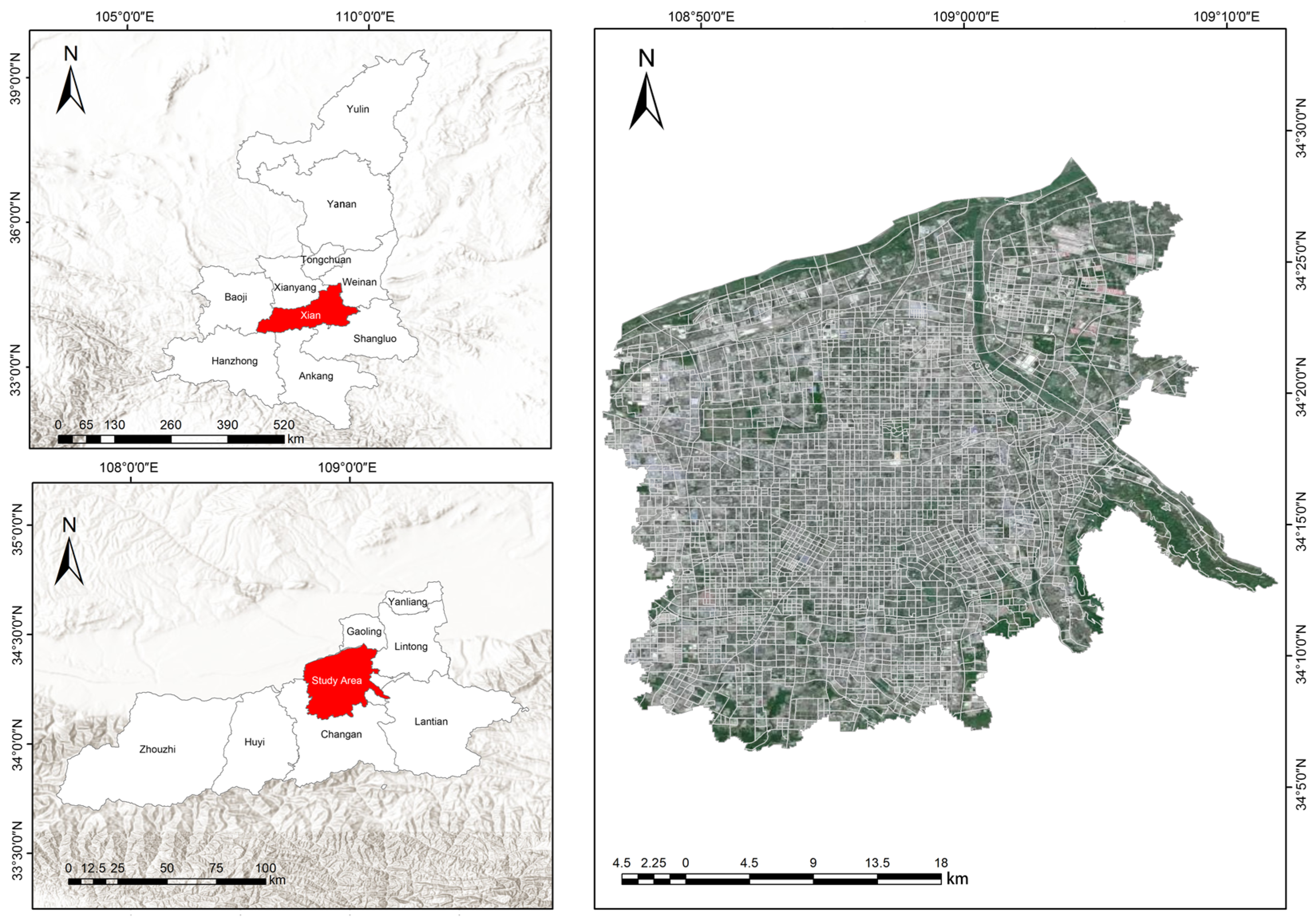
2.1. Summary of the Study Area

Xi’an, the provincial capital of Shaanxi, is situated in the northwestern region of China, on the central Guanzhong Plain. The City of Xi’an, as a megacity, has approximately 13.08 million permanent population by the end of 2023, covering an area of 10,096 square kilometers. As the ancient capital of thirteen dynasties in China and a crucial city in the Belt and Road Initiative, the core urban region of Xi’an demonstrates a pronounced population agglomeration effect, with dense commercial activity and notable variations in vitality. This study applies blocks as the basic units for analysis to reflect detailed and accurate spatial differences in urban vitality. It combines Xi’an’s OpenStreetMap road network data with remote sensing imagery to divide the central urban area into 3302 basic units (Figure 1).

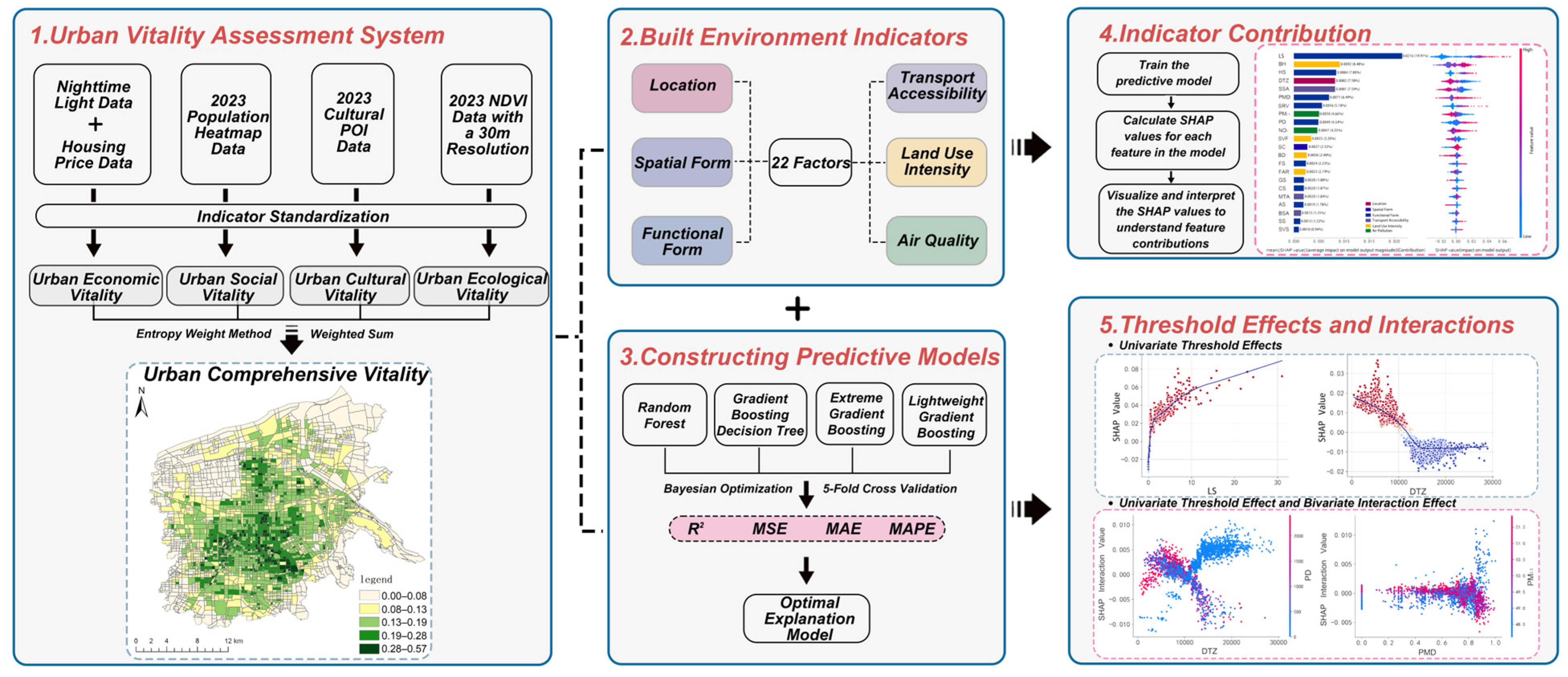
2.2. Research Framework and Data Collection and Pre-Processing

This study employs multi-source data to conduct a comprehensive assessment of Xi’an across four key dimensions: economic, social, cultural, and ecological. The vitality values corresponding to each dimension are standardized, after which the entropy weighting method is applied to derive a composite measure of urban vitality. A built environment indicator system is then developed, encompassing 22 carefully selected factors spanning six critical domains: location, spatial form, functional structure, transportation accessibility, land use intensity, and air quality. Furthermore, four advanced predictive models—RF, GBDT, XGBoost, and LightGBM—are trained, with the optimal model identified based on performance. Finally, this model is employed to quantify the nonlinear threshold effects and complicated interactions between built environment factors and spatial vitality. Figure 2 illustrates the workflow of this study.

This study primarily utilizes several datasets, including Baidu heatmaps, OSM road network data, POI data, housing price data, building vector data, GF-6 satellite imagery, nighttime light data, Landsat-8 remote sensing imagery, and air quality data (see

Table 1. Description of the dataset.

Dataset Name	Data Structure	Data Source	Description
Administrative Boundaries of Xi’an	Vector polygon data	https://www.webmap.cn/, accessed on 2 October 2024.	2023 data containing spatial information on Xi’an’s administrative boundaries
GF-6 Data	Raster data	https://www.cpeos.org.cn/, accessed on 2 October 2024.	High-resolution multispectral satellite imagery from 2023 with a spatial resolution of 8 m
Nighttime Light Data	Raster data	https://eogdata.mines.edu/products/vnl/, accessed on 8 October 2024.	2023 annual average nighttime light imagery with a spatial resolution of 500 m, used to represent human activity intensity
Landsat-8 Imagery Data	Raster data	https://landsat.gsfc.nasa.gov/satellites/landsat-8/, accessed on 10 October 2024.	2023 multispectral satellite imagery with a spatial resolution of 30 m
Baidu Heatmap Data of Xi’an	Raster data	https://map.baidu.com/, accessed on 16 October 2024.	2023 data, including building height and 2D footprint information within the study area
Building Vector Data	Vector polygon data	https://map.baidu.com/, accessed on 14 October 2024.	2023 Baidu heatmap imagery with a spatial resolution of 30 m
Road Network of Xi’an Central Urban Area	Vector line data	https://www.openstreetmap.org/, accessed on 5 October 2024.	2023 vector line data of major roads in Xi’an’s central urban area
POI Data of Xi’an Central Urban Area	Vector point data	https://lbs.amap.com/, accessed on 18 October 2024.	2023 data showing geographic locations and categories of public service facilities in the central urban area
Housing Price Data of Xi’an Central Urban Area	Vector point data	https://xa.anjuke.com/, accessed on 16 October 2024.	2023 geolocated point data of housing prices
Traffic Station Data of Xi’an Central Urban Area	Vector point data	https://lbs.amap.com/, accessed on 7 October 2024.	2023 point data of public transportation stations with an approximate spatial resolution of 500 m
Air Quality Data	Raster data	https://www.cnemc.cn/sssj/, accessed on 30 October 2024.	2023 annual average concentrations of air pollutants (PM2.5 and NO2) with a spatial resolution of 1000 m

). The Baidu heatmap data were obtained via the Baidu Huiyan API, capturing anonymized real-time mobile device activity. The data are aggregated hourly and averaged over the year, with a spatial resolution of approximately 30 m. Road network data were obtained from the OpenStreetMap (OSM) website and processed into road centerlines, followed by topological optimization. POI data were collected using web scraping techniques in combination with the Baidu Map and Amap (Gaode) APIs. The data include a variety of categories such as education, healthcare, commercial, and transportation facilities, and are detailed and represented as vector point data. Building data were similarly extracted from Amap using the same method. This data includes attributes such as building height and number of floors and is represented as vector polygon data. Housing price data for Xi’an were extracted from the Anjuke website using web scraping techniques, including geographic information in vector point format. The GF-6 satellite imagery was pre-processed to generate orthorectified images of the study area. The nighttime light data, with a spatial resolution of 500 m, were obtained from the Earth Observation Group platform, representing the average annual nighttime light levels for 2023. Additionally, ENVI 5.3.1 was employed to perform radiometric calibration and atmospheric correction on Landsat-8 imagery to derive the normalized difference vegetation index (NDVI) data. Finally, the air quality data were obtained from the China National Environmental Monitoring Center (CNEMC). Based on monitoring results from national environmental air automatic monitoring stations within the study area, spatial interpolation was performed to generate gridded data with a resolution of 1 km. The environmental parameters selected for this study primarily focus on the PM_2.5 and NO₂ concentrations within urban blocks, with annual average pollution levels used to analyze their impact on urban vitality.

2.3. Construction of Urban Vitality Factors

This study develops a comprehensive indicator system to evaluate urban vitality from four dimensions, relying on the precision, adaptability, and reliability of different data sources: economic, social, cultural, and ecological [40,41,42]. The dataset includes nighttime light data, housing price data, population heat maps, cultural POIs, and NDVI data.

2.3.1. Assessment of Urban Economic Vitality

Economic vitality is commonly represented by nighttime light intensity or the usage levels of various commercial facilities [2,21]. To capture long-term human activities in economic vitality, this study also supplements housing prices with nighttime light intensity in the evaluation process by applying entropy weighting [11]. This approach reflects the current level of economic activity in Xi’an and incorporates the market’s projections regarding future expansion and progress, offering a more holistic perspective on economic vitality [2,40].

$$E_i=\alpha \ast H_i+\beta \ast L_i$$

(1)

where $E_i$ represents the economic vibrancy value of the region, $\alpha$ and $\beta$ are the weighting coefficients assigned to the two factors by the entropy method, corresponding to $H_i$ and $L_i$, respectively. $H_i$ is the nighttime light data, and $L_i$ is the housing price data. The specific values are shown in

Table 2. Weights of vitality factors for different dimensions.

Vitality Dimensions	Data Types	Weights
Economic Vitality	Nighttime Light Data	0.102
	Housing Price Data	0.150
Social Vitality	Population Heatmap Data	0.366
Cultural Vitality	Cultural POI Data	0.300
Ecological Vitality	NDVI	0.082

.

2.3.2. Assessment of Urban Social Vitality

Urban social vitality is predominantly determined by human activities, positioning it as an essential constituent of overall urban vitality [43]. The data utilized to quantify this vitality is derived from the Baidu heatmap. It combines geographic spatial information with data, using visual encoding techniques such as color gradients and brightness variations to clearly illustrate data distribution patterns, significantly improving data readability and analysis efficiency [44]. In this study, Baidu heatmap data were collected from 7:00 to 22:00 on both 16 April and 17 April 2023. The heat index for each time period was calculated using inverse distance weighting interpolation, with the average heat index serving as an indicator of the social vitality of each block. The calculation formula is Equation (2) [1,15]:

$$Z_{x,y}={\displaystyle \frac{{{\displaystyle \sum }}_{i=1}^n{Z}_i{d}_{x,y,i}^{-\beta }}{{{\displaystyle \sum }}_{i=1}^n{d}_{x,y,i}^{-\beta }}}$$

(2)

where $Z_{x,y}$ represents the point to be estimated, $Z_i$ denotes the control value of the $i$-th sample point, and the parameter $\beta$ is the power parameter used to define the weight of each control point $Z_i$ in the interpolation process. d_x,y,i is the distance between $Z_{x,y}$ and $Z_i$.

2.3.3. Assessment of Urban Cultural Vitality

The existence and spatial arrangement of cultural facilities reflect the material needs of society amidst the continuous enhancement of social and cultural literacy, exhibiting distinct spatial characteristics [45]. Areas with a higher concentration of cultural facilities tend to experience more frequent cultural exchange activities, with greater potential for cultural participation and interaction. In this study, cultural and educational POIs are used for kernel density analysis to derive the cultural vitality index for each block, representing the level of cultural vitality (Equation (3)) [18]. Furthermore, after multiple experiments, the 500 m search radius is suitable for kernel density estimation.

$$f_n\left(x\right)={\displaystyle \frac{1}{n\pi r^2}}{\displaystyle \sum }_{i=1}^{n}K\left[1-\left({\displaystyle \frac{{\left(x-x_i\right)}^2+{\left(y-y_i\right)}^2}{r^2}}\right)\right]$$

(3)

where $f_n\left(x\right)$ represents the kernel density estimate at the spatial location ($x_i$, $y_i$), K denotes the kernel function, ${\left(x-x_i\right)}^2+{\left(y-y_i\right)}^2$ represents the search radius or kernel density bandwidth centered at ($x_i$, $y_i$), and $n$ signifies the number of sampling points within this radius.

2.3.4. Assessment of Urban Ecological Vitality

Higher environmental quality not only markedly boosts individuals’ tendency to participate in outdoor pursuits but also promotes greater diversity and engagement in social interactions, thereby boosting the comprehensive vitality of the city [23]. The normalized difference vegetation index (NDVI), a core indicator of vegetation coverage and health, is widely used in ecological environment assessments. NDVI values were extracted from high-resolution remote sensing imagery captured by the Landsat-8 satellite in April 2023 using ENVI 5.3.1 [41]. The formula for calculation is presented in Equation (4) [14,23]:

$$EV={\displaystyle \frac{{{\displaystyle \sum }}_{i=1}^{n}NDV{I}_i}{n}}$$

(4)

where $NDV{I}_i$ refers to the normalized difference vegetation index for each study block, n represents the count of pixels within the given neighborhood, and $EV$ represents the average normalized vegetation index for each community. $NDVI$ reflects biomass and vegetation vitality, with higher $NDVI$ values indicating greater vegetation coverage and higher biomass, suggesting stronger environmental vitality in the area.

2.3.5. Urban Comprehensive Vitality Assessment

To ensure uniformity in the assessment of vitality across various aspects, we standardized the economic, social, cultural, and ecological indices using min–max normalization [2]. Additionally, we employed the entropy weighting method to calculate the weights for each indicator [14,18]. The weights assigned to each of the four dimensions are presented in Table 2.

2.4. Influencing Factor Selection

To explain urban vitality, the intrinsic features and external conditions of urban blocks are examined, including location, spatial form, functional form, transportation accessibility, land use intensity, and air quality dimensions, identifying a total of 22 influencing factors. According to literature review [15,17,26], factors such as unit location (DTZ), spatial compactness (SC), points of interest (POI), accessibility (TA), floor area ratio (FAR), building density (BD), and average building height (BH) have been widely employed in developing built environment indicator systems. Building upon these factors, this study innovatively incorporates the openness of blocks’ visual perception and air pollution, including sky visibility factor (SVF), PM_2.5 concentration (PM_2.5), and NO₂ concentration (NO₂). For detailed information about the specific factors and the calculation process, please refer to

Table 3. A comprehensive built environment factor system.

I Influencing Factors	II Indicator	Abbreviation	Meaning (Unit)
Location	Block Location	DTZ	The distance from the block unit to the city center of Xi’an (km)
Spatial Form	Spatial Compactness	SC	The complexity of the spatial structure of the block unit
Functional Form	POI Mixing Degree	PMD	Reflecting the degree of mixing of points of interest (POI) within the block unit.
	POI Density	PD	Reflecting the number of points of interest (POI) within the block unit (count per 0.01 km2)
	Living Services	LS	Reflecting the number of various types of service facilities per unit area within the block (count per 0.01 km2)
	Healthcare Services	HS
	Financial Services	FS
	Catering Services	CS
	Accommodation Services	AS
	Shopping Services	SS
	Government Services	GS
	Sports-Related Services	SRV
	Scenic View Services	SVS
Transport Accessibility	Bus Stop Accessibility	BSA	The average total time spent traveling from the block unit to each bus stop (min)
	Subway Station Accessibility	SSA	The average total time spent traveling from the block unit to each subway station (min)
	Major Transportation Accessibility	MTA	The average total time spent traveling from the block unit to each major transportation hub (min)
Land Use Intensity	Building Density	BD	Reflecting the ratio of the building area to the block area within the block unit
	Floor Area Ratio	FAR	Reflecting the ratio of the total building area to the block area within the block unit
	Average Building Height	BH	Reflecting the average building height within the block unit (m)
	Sky View Factor	SVF	Reflecting the obstruction of the sky by buildings within the block unit
Air Quality	PM2.5 Concentration	PM2.5	The total number of particulate matter with a diameter less than or equal to 2.5 μm per unit volume within the block (μg/m3)
	NO2 Concentration	NO2	The proportion of NO2 molecules in the air relative to the total gas volume per unit volume within the block (μg/m3)

and Appendix A 

Table A1. Formulas and symbol definitions for built environment factors.

Abbreviation	Formula	Symbol Meaning	References
DTZ	/	/	[2]
SC	$SC={\displaystyle \frac{2\sqrt{\pi \ast {\mathrm{Area}}_{\mathrm{i}}}}{L}}$	Areai refers to the area of the i-th urban block, and L represents the perimeter length of its administrative boundary.	[14]
PMD	$PMD=1-{{\displaystyle \sum _{\mathrm{i}=1}^{\mathrm{n}}\left(\frac{P_{\mathrm{i}}}{P_{\mathrm{total}}}\right)}}^2$	Pi indicates the count of points of interest (POIs) in the i-th category, while Ptotal denotes the total number of POIs within the block. The variable n represents the number of POI categories (e.g., dining, education, healthcare).	[18]
PD	$PD={\displaystyle \frac{N_{\mathrm{i}}}{{\mathrm{Area}}_{\mathrm{i}}}}$	Ni represents the total count of point of interest (POI) facilities in block i.	[41]
LS	$S{F}_{\mathrm{i}}={\displaystyle \frac{{\mathrm{n}}_{\mathrm{i}}}{{\mathrm{Area}}_{\mathrm{i}}}}$	SFi indicates the service facility density for each POI category. ni represents the total number of POI facilities of a given type (such as catering, educational, or medical services) within block i.	[2,42]
HS
FS
CS
AS
SS
GS
SRV
SVS
BSA	$T={\displaystyle \frac{{\displaystyle {\sum }_{\mathrm{i}=1}^{\mathrm{n}}{\mathrm{t}}_{\mathrm{ij}}}}{\mathrm{n}}}$	T represents the mean travel time from the block to a set of relevant transport stations, and tij denotes the travel time from block i to station j. The variable n refers to the total number of such stations, including bus stops, subway stations, and large-scale transit hubs.	[14]
SSA
MTA
BD	$BD={\displaystyle \frac{{\displaystyle {\sum }_{\mathrm{i}=1}^{\mathrm{n}}{A}_{\mathrm{i}}}}{A{\mathrm{rea}}_{\mathrm{i}}}}$	Ai represents the ground coverage area of buildings in the block, with n indicating the total number of buildings contained within the block.	[18]
FAR	$FAR={\displaystyle \frac{{\displaystyle {\sum }_{\mathrm{i}=1}^{\mathrm{n}}{A}_{\mathrm{i}}\times F_{\mathrm{i}}}}{A{\mathrm{rea}}_{\mathrm{i}}}}$	n refers to the total number of buildings in the block, Ai denotes the ground coverage area of the i-th building, and Fi indicates its number of floors.	[18]
BH	$BH={\displaystyle \frac{{\displaystyle {\sum }_{\mathrm{i}=1}^{\mathrm{n}}{H}_{\mathrm{i}}}}{\mathrm{n}}}$	n refers to the total number of buildings in the block, while Hi indicates the height of the i-th building within the block unit.	[41]
SVF	$\mathrm{SVF}=1-{\displaystyle \frac{{\displaystyle {\sum }_{\mathrm{i}=1}^{\mathrm{n}}{\sin \mathrm{\gamma }}_{\mathrm{i}}}}{\mathrm{n}}}$	γi represents the elevation angle of the terrain horizon in the i-th direction, and n denotes the number of directions used to estimate γ.	[32]
PM2.5	$C={\displaystyle \frac{M}{V}}$	C indicates the concentration of the corresponding pollutant, M represents the mass of the pollutant captured during the sampling process, and V refers to the volume of the collected sample. (In this study, the pollutants specifically refer to PM2.5 and NO2.)	[38,59]
NO2

.

2.5. Machine Learning Models

To investigate the driving mechanisms through which built environment factors influence urban vitality, this study introduces four machine learning (ML) models to estimate the marginal effects of various factors and to explore the compound effects arising from interactions among multiple variables. The models—random forest (RF), gradient boosted decision trees (GBDT), extreme gradient boosting (XGBoost), and light gradient boosting machine (LightGBM)—are equipped with strong nonlinear modeling capabilities and the ability to evaluate variable importance. These models are well-suited to handle complex urban spatial data structures and to identify key influencing factors along with their impact pathways on urban vitality [36,37]. RF is an ensemble learning technique that constructs a set of decision trees with strong generalization capacity by employing bagging integration and random feature sampling. It enhances the diversity of machine learning models and effectively mitigates overfitting during data analysis [46]. GBDT is an iterative ensemble learning method based on decision trees that generate predictions by building a sequence of weak decision trees and combining their outcomes. By combining the concepts of boosting and decision trees, each iteration aims to fit the residuals from the previous round, progressively improving overall prediction accuracy [47]. XGBoost is derived from the gradient boosting decision tree method. It adds regularization terms to prevent overfitting and uses a second-order Taylor expansion, which is more accurate than the first-order derivatives used in GBDT, thereby improving the model’s ability to capture nonlinear relationships [48]. LightGBM is designed to handle massive spatiotemporal data. It incorporates strategies like one-sided gradient sampling and feature bundling, which provide excellent performance when processing large-scale data [49]. To comprehensively evaluate the models, the study calculates MAE, MSE, RMSE, and R² metrics to identify the best predictive model, which means a model with lower MAE, MSE, and RMSE, and higher R² would be selected for further analysis. Additionally, Bayesian optimization, along with five-fold cross-validation, was employed for hyperparameter adjustment to determine the optimal set of parameters [38].

In this study, we explain the LightGBM model using its formula as an example (formulas for the other three models can be found in the studies mentioned above). LightGBM is an efficient gradient-boosting tree algorithm, and its objective is to minimize the following objective function:

$$L\left(f\right)={\displaystyle \sum }_{i=1}^N\mathcal{l}\left(y_i,f\left(x_i\right)\right)+\Omega \left(f\right)$$

(5)

where the loss function $\mathcal{l}\left(y_i,f\left(x_i\right)\right)$ measures the deviation between the predicted value $f\left(x_i\right)$ and the true value $y_i$, the regularization term $\Omega \left(f\right)$ regulates model complexity to reduce the risk of overfitting.

For regression problems, the loss function is typically represented in the form of mean squared error (MSE):

$$\mathcal{l}\left(y_i,f\left(x_i\right)\right)={\left(y-f\left(x\right)\right)}^2$$

(6)

The model is trained by iteratively updating the tree structure. In each iteration, the model’s predictions are updated as specified by the following formula:

$$f^{\left(k\right)}\left(x\right)=f^{\left(k-1\right)}\left(x\right)+\eta \cdot h^{\left(k\right)}\left(x\right)$$

(7)

where $\eta$ represents the learning rate, and $h^{\left(k\right)}\left(x\right)$ denotes the decision tree generated during the kth iteration.

The tree splitting is based on a gain criterion, where the optimal splitting feature is determined by maximizing the gain value after each split. The formula for the tree split gain is as follows:

$$Ga\mathrm{i}n\left(t\right)={\displaystyle \frac{1}{2}}\left[{\displaystyle \frac{{\left({\Sigma }_{iϵL}{g}_i\right)}^2}{{\Sigma }_{iϵL}{h}_i+\lambda }}+{\displaystyle \frac{{\left({\Sigma }_{iϵR}{g}_i\right)}^2}{{\Sigma }_{iϵR}{h}_i+\lambda }}-{\displaystyle \frac{{\left({\Sigma }_{iϵL\cup R}{g}_i\right)}^2}{{\Sigma }_{iϵL\cup R}{h}_i+\lambda }}\right]$$

(8)

where $g_i$ and h_i represent the first- and second-order gradient statistics of the loss function, respectively, and $L$ and $R$ correspond to the left and right branches of the sample sets, respectively.

In order to better understand the complex influence of built environment factors on urban vitality, this study applies the SHAP interpretation approach. This method primarily calculates the marginal impact of each feature on the model’s output, as well as the interactions between multiple variables on urban vitality, providing interpretations from both global and local perspectives. It is based on cooperative game theory and serves as a post hoc explanation method for the model [1]. The detailed calculation procedure is outlined as follows:

$$SHA{P}_j={\displaystyle \sum }_{S\subseteq \left\{V_1,V_2,\dots ,V_p\right\}\setminus \left\{V_j\right\}}{\displaystyle \frac{\left|S\right|!\left(P-\left|S\right|-1\right)!}{P!}}\left[f_x\left(S\cup \left\{V_j\right\}\right)-f_x\left(S\right)\right]$$

(9)

$$y_i=y_{base}+{\Sigma }_{j=1}^{k}SHAP\left(x_{ij}\right)$$

(10)

where $SHA{P}_j$ denotes the $SHAP$ value of sample i for feature $j$; $S$ represents the subset of features utilized by the model; V_p refers to the set of all model features; $P$ is the total number of features; $f_n(x)$ signifies the model’s prediction based on the subset of features; $y_{base}$ represents the mean prediction value across the other samples; y_i refers to the predicted outcome for the specific sample $i$; and $k$ represents the total count of features. The sign of $SHAP\left(x_{ij}\right)$ reflects the specific impact of different urban characteristics on the predicted outcome. SHAP values use an additive approach to attribute the prediction, aggregating the contributions of each input feature to explain the model’s output.

3. Results

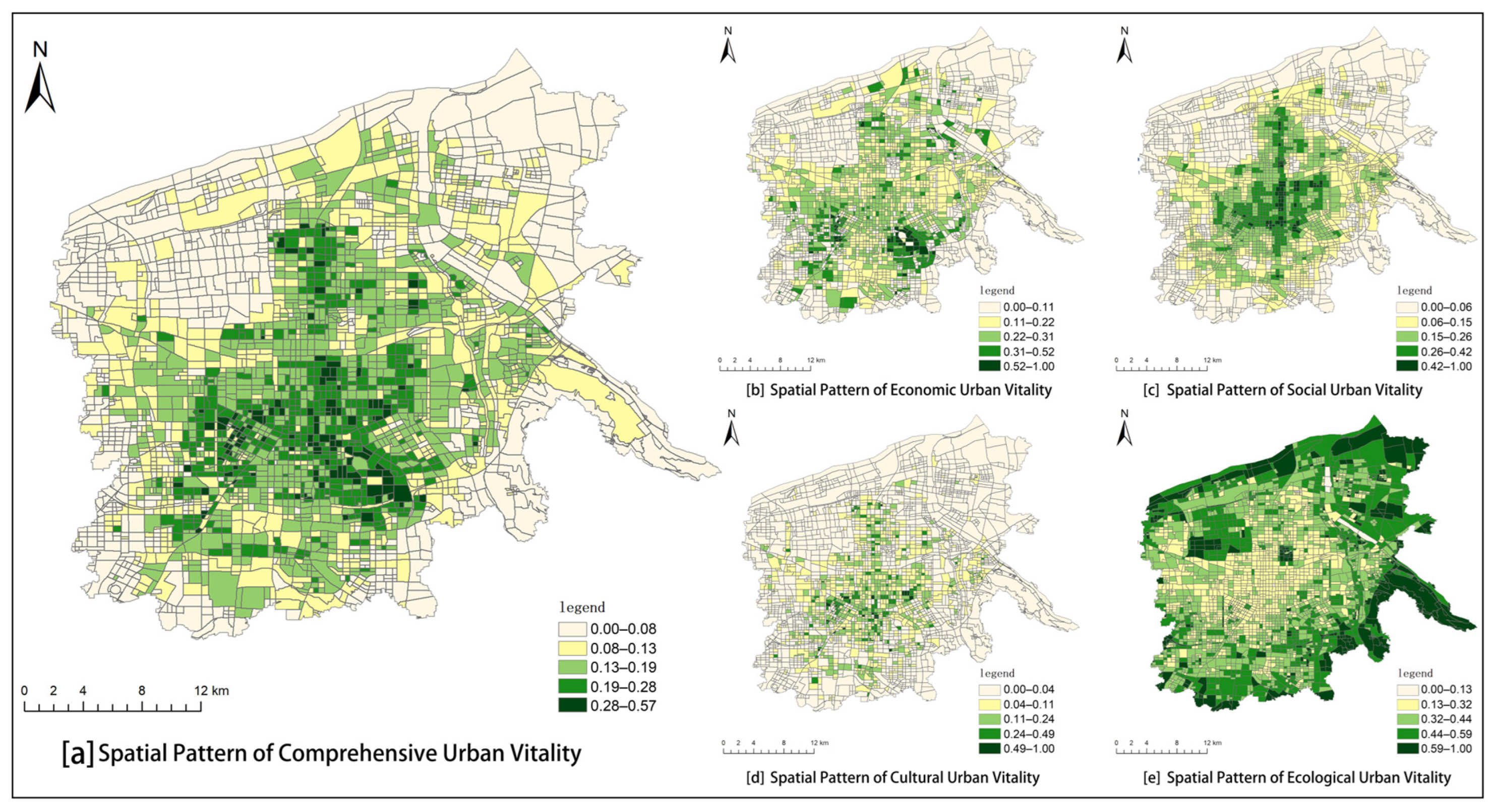
3.1. The Distribution Characteristics of Urban Vitality Across Different Dimensions

High economic vitality values exhibited a core aggregation pattern (Figure 3). By comparison, the distribution of social vitality followed a multi-center nested structure. Blocks with high cultural vitality formed a “V”-shaped distribution along the Ming Dynasty City Wall. In contrast, areas with high ecological vitality were concentrated at the edges of the central urban area, forming a circular distribution. Specifically, high economic vitality values are densely concentrated within the traditional commercial areas inside the city wall and the high-tech district (the CBD of Xi’an; vitality value > 0.52). A secondary vitality belt extended along main roads such as Weiyang Road and Chang’an Road, with color gradients transitioning from dark to light (vitality value 0.31–0.52). In contrast to economic vitality, social vitality showed multiple independent dark patches in emerging residential areas like Qujiang New District (vitality value 0.42–1.00), with a secondary vitality belt (0.26–0.42) surrounding these areas in a transitional manner, forming a “core-edge” nested pattern. Cultural vitality formed a continuous band of high-value dark areas (vitality value 0.49–1.00) around the cultural heritage zones near the Ming Dynasty City Wall (Beilin District, Big Wild Goose Pagoda), contrasting sharply with the surrounding light-colored regions (vitality value < 0.40). In contrast, high ecological vitality zones in the central urban area, such as Qujiang Pool and Xingqing Palace Park, appeared as isolated dark green patches (vitality value > 0.59), surrounded by low-value gray built-up areas (vitality value < 0.30). The peripheral high-value zone at the northern foot of the Qinling Mountains was similarly encircled by a low-value light green transition belt (vitality value 0.30–0.50), which includes areas along Huan Mountain Road (S107) and the buffer zone formed by the Xi’an-Chengdu high-speed railway passing through the Qinling section (Figure 3).

The results from the comprehensive spatial vitality distribution map of Xi’an clearly showed a ring-layer differentiation pattern in urban vitality. High-vitality core areas (0.28–0.57) were primarily located around transportation hubs such as the Bell Tower, the Xiaozhai commercial district, and Xi’an North Railway Station. The peak vitality value (0.57) arises from the combined effect of commercial complex clustering and the synergistic presence of cultural landmarks, such as the Tang Dynasty Evernight City. A secondary vitality belt (0.19–0.28) stretched along major roads, including Chang’an Road and Weiyang Road. This belt benefits from the mixed-use development pattern in the Qujiang New District and the high-tech district, showing a gradual decline in vitality values. It is worth noting that most urban villages, such as Shajing Village and Bali Village, are typically located in this transitional belt. Due to the concentration of migrant populations and the presence of small-scale commercial activities, these areas exhibit higher vitality than traditional industrial zones and protected areas. While their vitality remains lower compared to core areas, they still demonstrate a relatively significant level of urban vitality. Low-vitality areas (0.13–0.19) along the Third Ring Road were characterized by discontinuous strip-like distributions. These areas were mainly found in the Sanqiao area of Weiyang District, the extension of the Electronics Town in Yanta District, and the outer fringes of the Textile Town in Baqiao District. The distribution of these low-vitality zones aligns closely with the southwest–northeast urban expansion direction. The lowest vitality edge zones (0.00–0.13) were predominantly formed by the Qinling northern foothill protection area and traditional industrial zones like the Textile Town.

3.2. Mechanisms of the Influence of the Built Environment on Urban Comprehensive Vitality

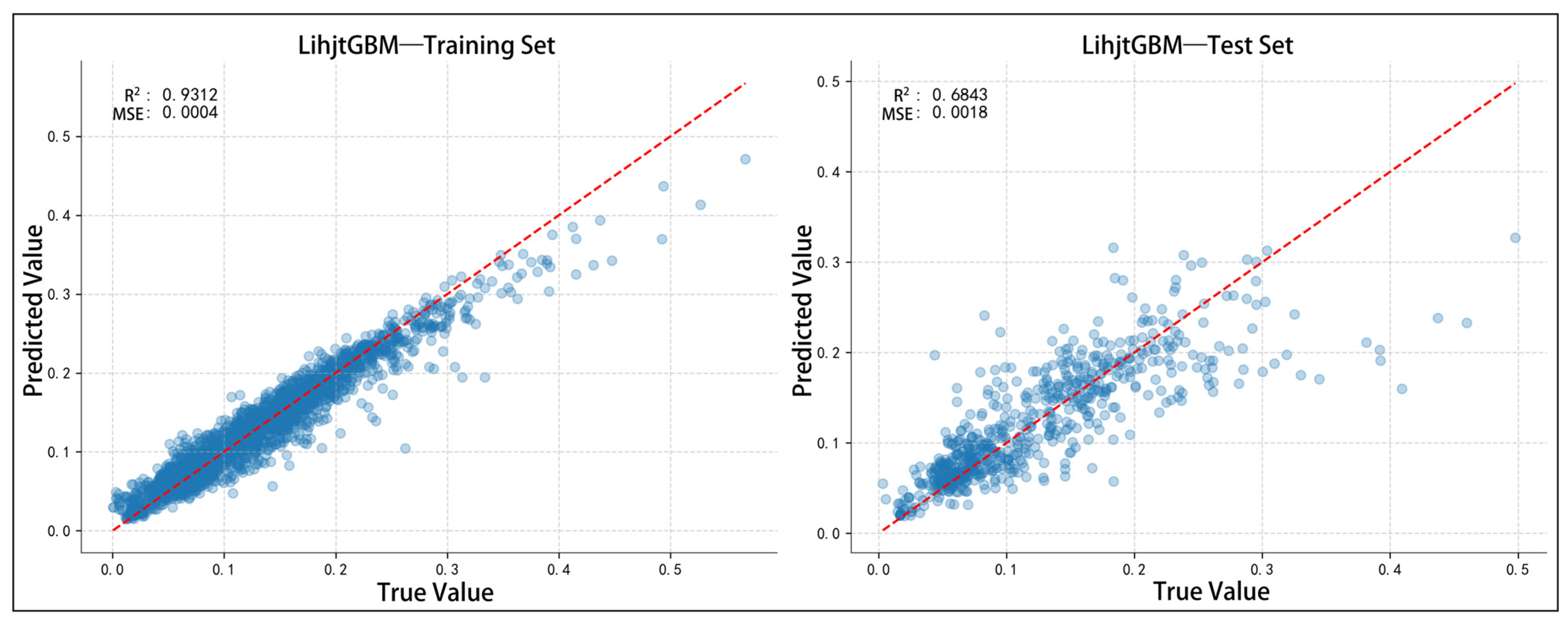
3.2.1. Optimal Model Validation

During the machine learning model fitting process, the dataset was randomly divided into training and testing sets in an 8:2 ratio, given the absence of significant temporal or spatial dependencies in the data. Specifically, 80% of the data was used for model training and validation, while the remaining 20% was reserved as the testing set to ensure fairness and representativeness in model evaluation [14]. The predictive performance of each model is evaluated using four metrics: R², MSE, MAE, and MAPE (

Table 4. Performance of four machine learning algorithms.

Model	R2	MSE	MAE	MAPE (%)
Random Forest	0.6648	0.0019	0.0285	20.1679
XGBoost	0.6739	0.0018	0.0280	19.5884
LightGBM	0.6843	0.0017	0.0277	19.1399
GBDT	0.6735	0.0018	0.0288	21.6456

Notes: R²: coefficient of determination, MSE: mean squared error, MAE: mean absolute error, and MAPE: mean absolute percentage error.

).

Four machine learning models demonstrated strong performance, but the LightGBM model excelled in R², MSE, and MAE metrics. It had the highest R² value (0.6829), indicating that the model explains the highest proportion of the variance in the target variable. Additionally, its MSE (0.0017), MAE (0.0276), and MAPE (19.1399%) were the smallest, signifying the lowest prediction errors. Therefore, the LightGBM model will be used to investigate the relative importance and nonlinear relationships between building environmental factors and urban vitality. The LightGBM model exhibited strong fitting performance on both the training and test sets (Figure 4). The model maintained high fitting accuracy on the training set (R² = 0.9312) and the test set (R² = 0.6843), with no evident signs of overfitting or underfitting. This further confirms its robustness.

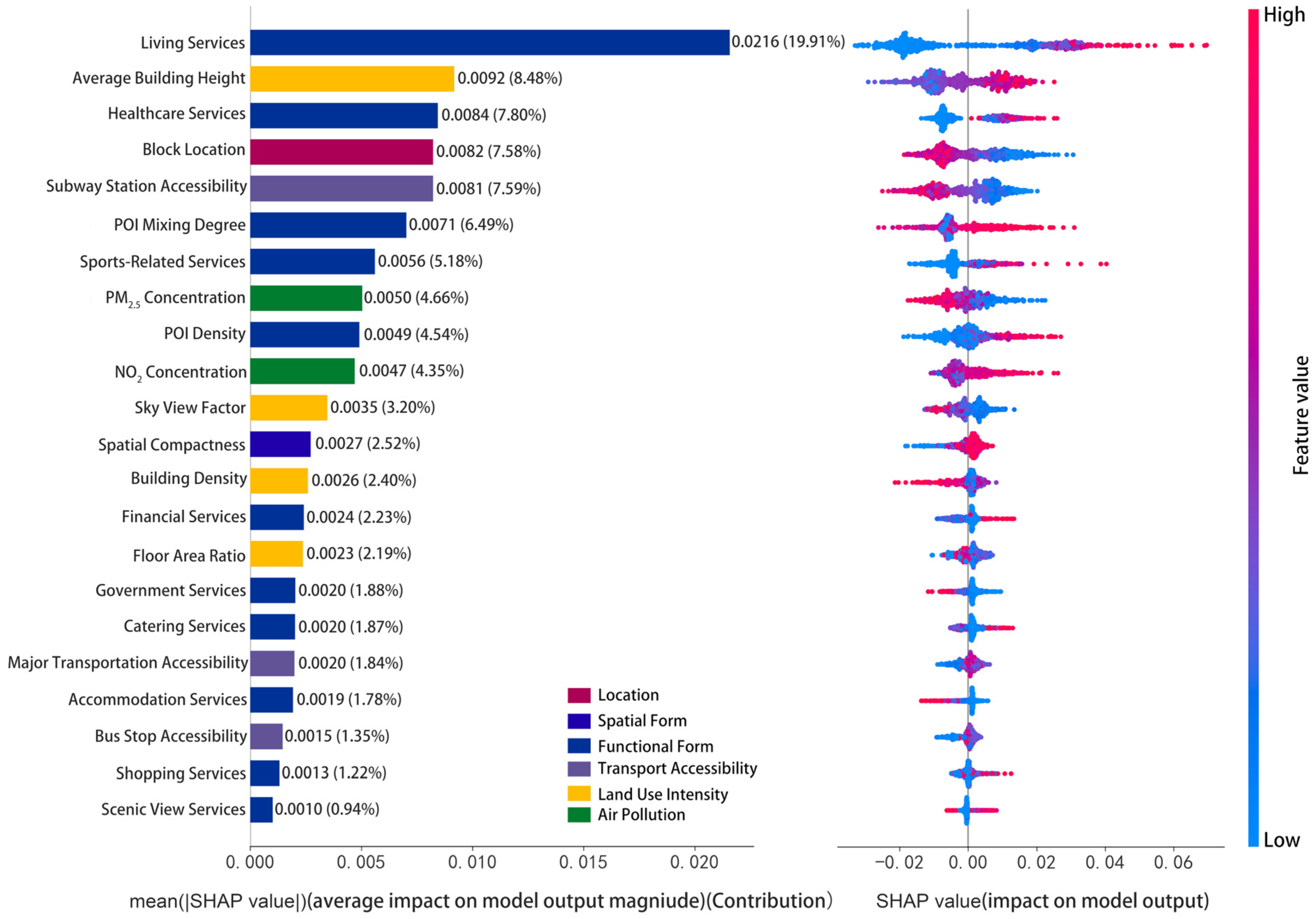
3.2.2. Relative Contributions of Different Influencing Factors

To identify the key characteristics influencing urban vitality, this study ranks the relative importance of influencing factors using SHAP (Figure 5). On the left, the importance of various factors within the built environment is presented, along with their specific relative contributions. These factors were ordered by descending importance, with colors representing the classification of factors into six distinct dimensions. On the right, the contribution of each factor to urban vitality was highlighted, with points ranging from red to blue, reflecting a gradient of feature values from high to low. The SHAP values along the horizontal axis reflect the negative and positive effects on the vitality of urban blocks.

In the built environment system, the functional morphology dimensions, including LS (living services), HS (medical services), SRV (sports services), and PMD (POI mix density), along with land use intensity variables such as BH (average building height), SVF (sky visibility), spatial morphology variable SC (spatial compactness), and the air pollution dimension NO₂ (NO₂ concentration), all demonstrated a significant positive influence on urban vitality. The cumulative contribution of these variables reached 59.27%, with LS, BH, and HS being the top three contributors, at 19.91%, 8.48%, and 7.80%, respectively. This suggests that areas with richer life services, improved medical facilities, and higher average building heights tend to exhibit higher urban vitality.

However, variables such as DTZ (block location), SSA (subway station accessibility), SVF (sky visibility), and PM_2.5 (PM_2.5 concentration) showed a significant negative impact on urban vitality, accounting for 23.05% of the total contribution. Among these, DTZ, with a contribution of 7.60%, had the most significant negative effect, indicating that the further a location is from the city center, the lower the urban vitality. Similarly, SSA, contributing 7.59%, highlighted the significant impact of longer commute times to public transport, subway, or major stations, which resulted in lower vitality. Conversely, the remaining ten variables, such as BD (building density), BSA (bus stop accessibility), AS (accommodation services), FS (financial services), and SVS (scenic view services), exhibited relatively lower importance, with a total contribution of just 17.68%, suggesting that their influence on urban vitality is relatively limited.

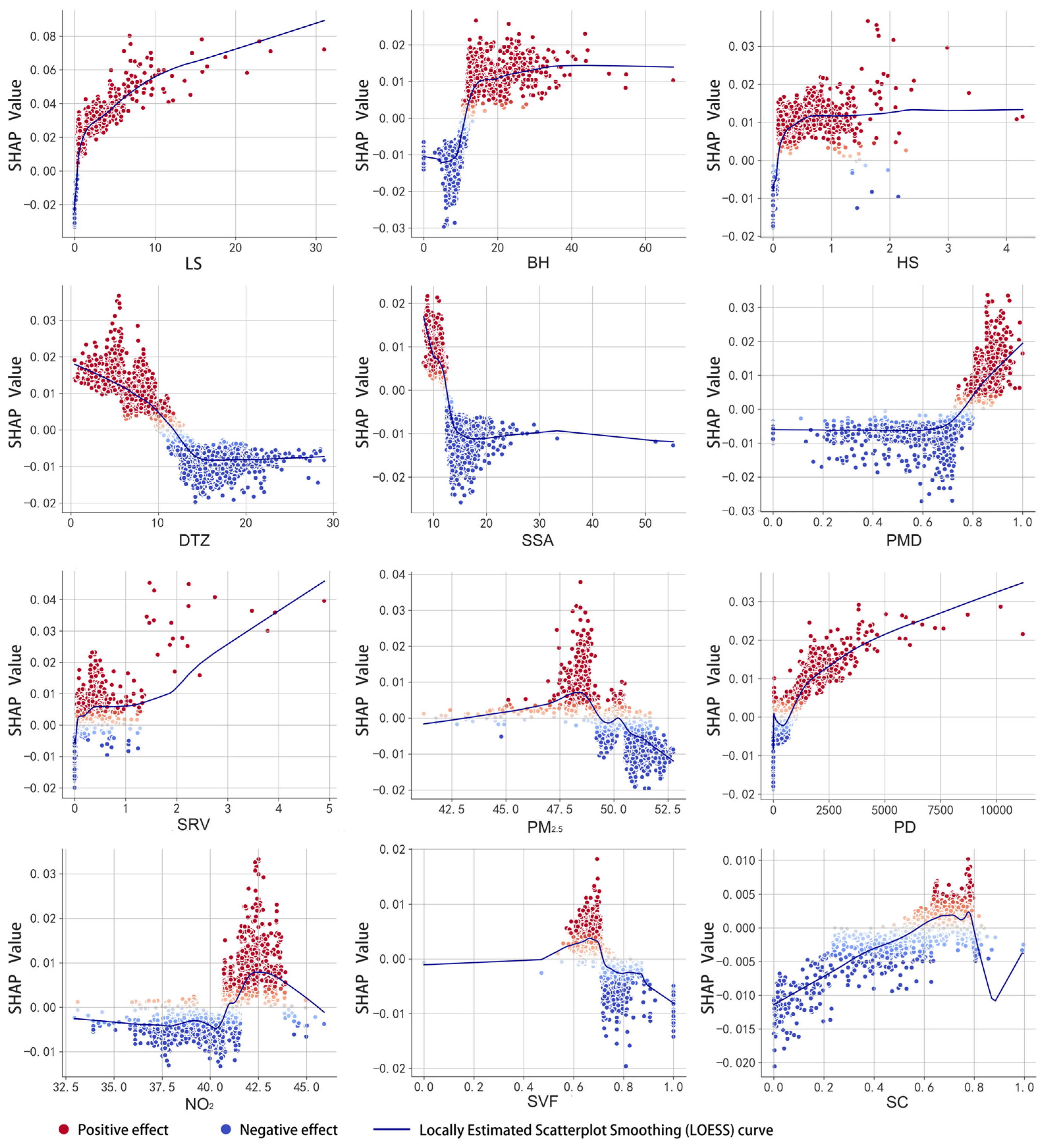
3.2.3. The Threshold Effects of Built Environment Factors

The nonlinear impacts of built environment factors on block-level urban vitality were illustrated using SHAP dependence plots (Figure 6), where the horizontal axis represents the values of each factor and the vertical axis indicates their contribution to overall vitality. A value above zero on the vertical axis denotes a positive impact on vitality, while a value below zero indicates a negative impact. To better visualize the nonlinear relationships and threshold effects between variables and urban vitality, the LOESS (locally weighted scatterplot smoothing) method was applied to smooth the scatter data. This technique effectively captures local trends without relying on the structural assumptions inherent in traditional global regression models, thereby providing a more accurate depiction of the threshold effects associated with each influencing factor [50].

The study conducted threshold analysis on the top twelve factors, which collectively accounted for more than 80% of the total contribution. Among these, LS (living services) and PD (POI density) exhibit similar trends, both having a highly significant positive impact on urban vitality. When their feature values are ≥1, urban vitality increases rapidly as the indicator values rise. PMD (POI mixing degree), which reflected block POI diversity, had a weaker effect on comprehensive vitality in the initial stages (feature values between 0 and 0.7). However, once the PMD value exceeded the threshold of 0.7, its contribution to vitality increased substantially. This finding suggests that richer life services and greater functional diversity contribute to higher urban vitality. In contrast, DTZ (block location) and SSA (subway station accessibility) demonstrated varying effects within different ranges. DTZ had a positive impact on vitality when its feature value was between 0 and 10. However, once it surpassed 12, its contribution to vitality gradually weakened, turning negative after exceeding 15, and stabilizing. Similarly, SSA showed a positive influence on vitality between feature values of 8 and 12, but once it surpassed the threshold of 12, it began to negatively affect vitality and stabilize. The relationship between BH (building height) and urban vitality also revealed a clear threshold effect. Below the threshold of 15, the effect was negative. Once the value exceeds 15, building height positively influences urban vitality, stabilizing after reaching the threshold of 32. This indicates that moderate increases in building height can stimulate urban vitality, but the effect plateaus beyond a certain height.

Additionally, the effects of HS (healthcare services) and SRV (sports-related services) service facilities on urban vitality differed. While both generally exert a positive impact on urban vitality, their rates of convergence vary. HS experienced a slight reduction in its contribution to vitality once its value reached 1, but it had a positive effect and stabilized thereafter. In contrast, SRV significantly enhanced its contribution to vitality once the feature value exceeded 2, with this positive effect continuing to strengthen. SC (spatial compactness) and SVF (sky view factor) also displayed distinct patterns in the plot. SC followed an inverted “U” shape, showing a negative impact on urban vitality when its feature value was below 0.6. As the SC value increased, the negative effect gradually diminished, but once the threshold of 0.7 was reached, SC’s impact on vitality shifted from a slight positive to a negative effect. SVF exhibited a weak, slightly positive contribution when its feature value was below the threshold of 0.72, but beyond this point, its contribution declined and became slightly negative. A similar trend was observed with PM_2.5, which transitions from a mildly positive impact on vitality to a negative one once the threshold of 47.5 is surpassed. In contrast, NO₂, an air quality indicator, enhanced urban vitality when exceeding 40.5, peaked at 42.5, then gradually declined, with higher values eventually leading to a negative impact.

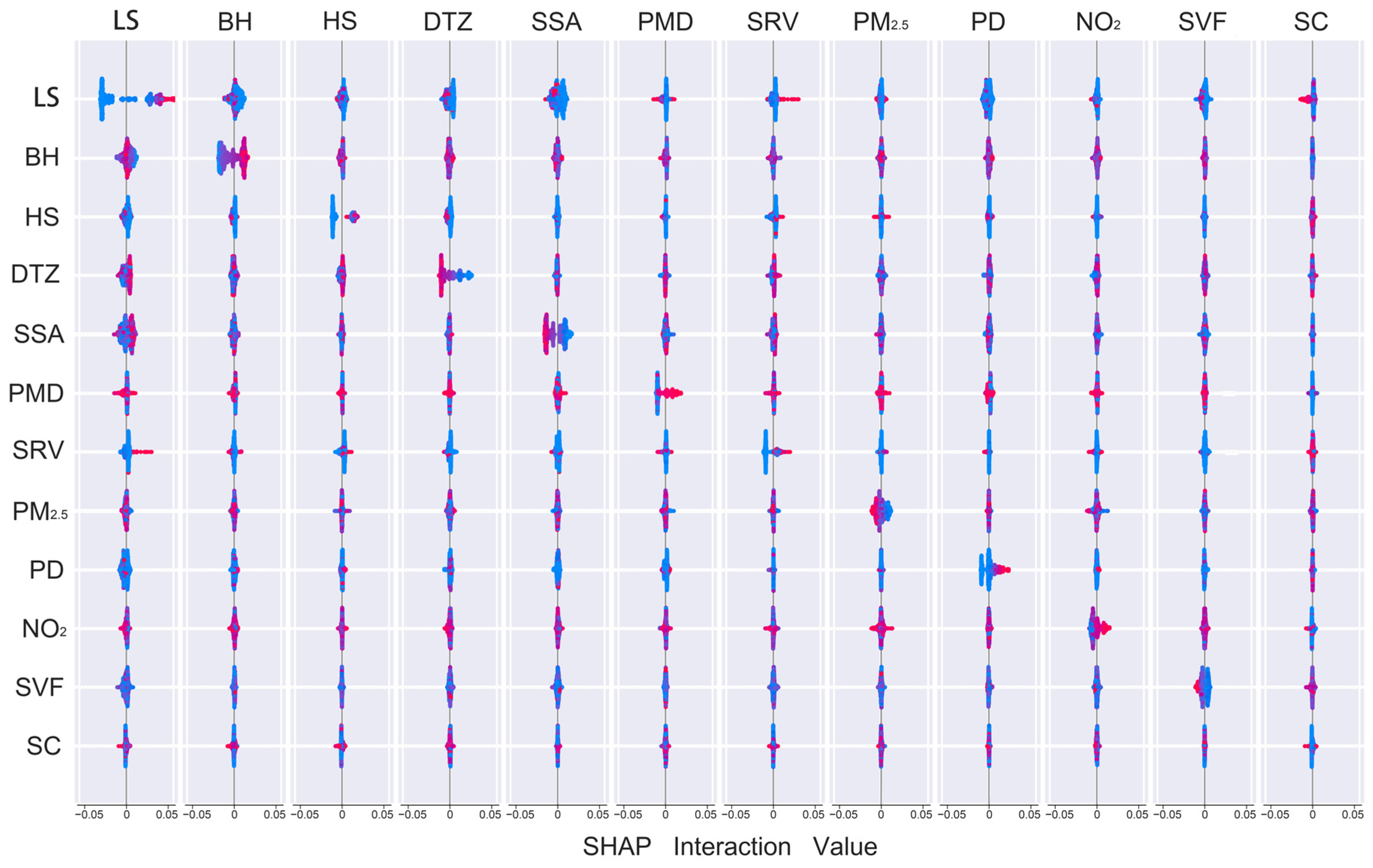
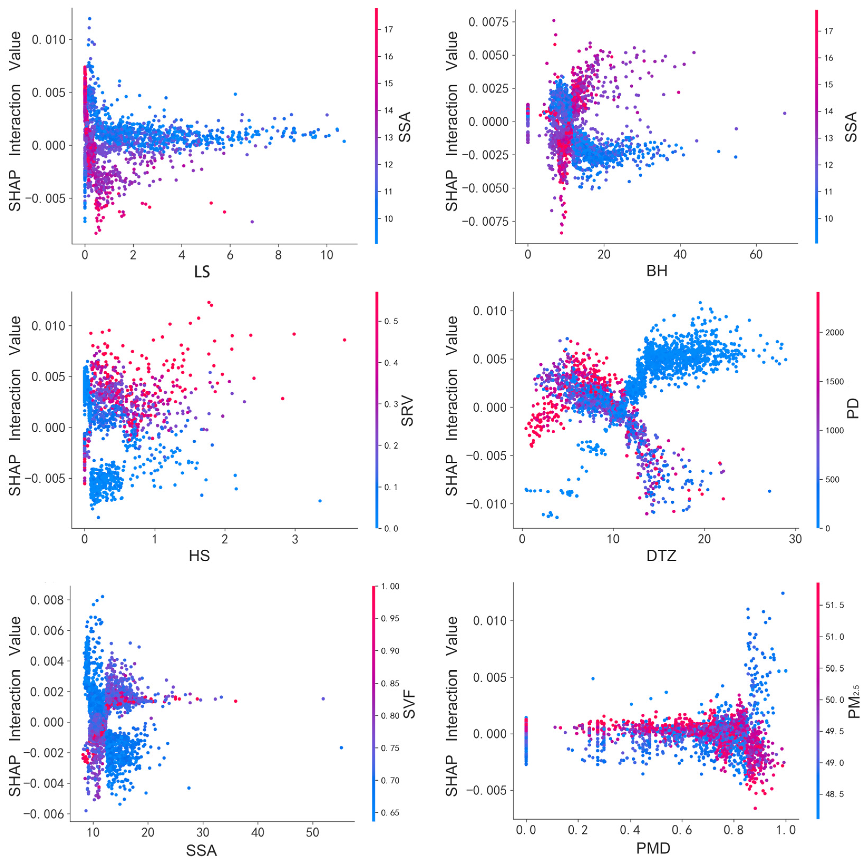
3.2.4. Interactions of Influencing Factors

In the SHAP model, the effect of each influencing factor variable on urban vitality is divided into main effects and interaction effects. The study computed the Shapley interaction values for each pair of variables and presented an interaction matrix plot (Figure 7), which included the top 12 variables contributing over 80% of the total contribution. Each plot represents a unique pair of variables, illustrating how they jointly affect urban vitality. On the left side of each plot, the selected variable is shown, with red indicating high values and blue indicating low values. The top side represents the second interacting variable. The x-axis is used to represent the Shapley interaction values between the two variables, where negative values correspond to inhibitory effects and positive values correspond to promotive effects on vitality.

To further investigate the combined effects of two factors on urban vitality, the study selected six key variables (LS, BH, HS, DTZ, SSA, and PMD) that exhibited the highest contributions to overall vitality, and analyzed their interactions with the variables showing the most significant interactive influence. Interaction plots were used to illustrate how pairs of variables jointly modulate their contributions to urban vitality. In each plot, the x-axis represents the value range of the selected primary variable, the color gradient indicates the value variation of the interacting variable, and the y-axis reflects the direction and magnitude of their joint contribution to urban vitality (Figure 8).

The results indicated that blocks with more comprehensive life services and those closer to subway stations positively influence urban comprehensive vitality. However, as the number of life service facilities increased (LS value ≥ 2) and the average time to the subway station decreased (SSA value ≤ 12), the synergistic effect of these two factors on vitality gradually weakened. Furthermore, when the average travel time to the subway station was high (SSA value ≥ 15), irrespective of the density of life service facilities, a suppressive effect on urban vitality was observed. In contrast, when the average building height (BH value ≥ 18) or sky view factor (SVF ≥ 0.75) is relatively high, blocks exhibit a positive impact on urban vitality despite longer commute times to metro stations; however, blocks closer to metro stations show a negative effect. This may be because spatial environments with open views can partially compensate for the lack of metro accessibility, while areas near metro stations with such spatial characteristics may experience suppressed urban vitality due to excessive functional concentration and environmental congestion.

In terms of medical resources and sports facilities, when both reached medium to high levels (HS value ≥ 1 or SRV value ≥ 0.3), they exerted a slight positive effect on urban vitality. However, in blocks with inadequate medical resources (HS value ≤ 0.6) and insufficient sports facilities (SRV value ≤ 0.2), the misallocation of resources resulted in a decline in public space utilization efficiency, which suppressed block vitality. The interaction between the distance to the city center (DTZ) and POI facility density (PD) exhibited significant spatial differentiation. When blocks were close to the city center (DTZ value ≤ 10) and had high POI density (PMD value ≥ 7), these factors positively interacted to enhance vitality. Conversely, blocks located farther from the city center (DTZ value > 10) with high POI density (PMD value > 7) negatively impacted vitality. This suggests that POI distribution in areas distant from the city center may fail to attract sufficient pedestrian flow, leading to resource inefficiencies and decreased vitality. When the block’s POI diversity was high (PMD value ≥ 0.8) and the PM_2.5 concentration was low (PM_2.5 value ≤ 49.5), the interaction between these factors had a significant positive effect on urban vitality. However, as the PM_2.5 concentration rose (PM_2.5 value ≥ 50.5), the SHAP interaction value between POI diversity and PM_2.5 concentration consistently turned negative. This indicates that the positive impact of POI diversity on urban vitality is significantly diminished as air pollution levels increase, highlighting the moderating role of air quality in shaping the relationship between POI diversity and urban vitality.

4. Discussion

4.1. Spatial Patterns of Urban Vitality

Vitality across different dimensions in the central urban area of Xi’an exhibits distinct stratification and regional characteristics, reflecting both synergies and conflicts [51,52]. From an economic perspective, the high-value economic vitality areas, such as the traditional commercial districts within the Ming Dynasty City Wall and the High-Tech Zone, primarily rely on the agglomeration of the tertiary industry and high transportation accessibility, which facilitate substantial flows of capital and population [53,54]. The distribution of social groups reveals a diverse pattern of interactions and clustering in the central area. Due to their high historical value and concentration of entertainment and public service facilities, the Qujiang New District and blocks near the Bell Tower have become social vitality hotspots. Conversely, traditional industrial zones, such as the Textile Town, exhibited low social vitality due to insufficient public spaces and population aging issues, highlighting the key role of improving public services and optimizing population structure in boosting social vitality [55]. In terms of cultural vitality, emerging cultural hubs on the outskirts fail to achieve effective clustering due to their limited functions and low activity levels, reflecting the tension between cultural heritage preservation and modern development. Regarding ecological vitality, marginal areas show significant erosion, with urban expansion negatively impacting green buffer zones and reducing ecological regions of the central city, highlighting the insufficient provision of environmental services in the context of high-density development [56].

Overall, the comprehensive vitality of Xi’an displayed a multi-layered and multi-center interlinked spatial pattern. Central areas such as the Bell Tower, Xiaozhai Commercial District, Qujiang New District, and major transportation hubs like Xi’an North Railway Station exhibited exceptionally high vitality (0.57). These areas stand out due to their concentration of commercial, cultural, and tourism resources, coupled with accessible transportation facilities. These factors collectively facilitate the concentration and mobility of resources and population, thereby contributing to the formation of dynamic core zones. In contrast, regions such as the western part of Weiyang District, the eastern part of the Chanba Ecological Zone, and the Caoshan Industrial Area, characterized by outdated public services and limited functions, exhibited low comprehensive vitality (0.00–0.13).

4.2. Threshold Effects and Interactions of the Built Environment on Urban Vitality

4.2.1. Nonlinear and Threshold Effects of Individual Variables on Urban Vitality

The findings of this study align with the views of Zheng and Yang, both of which indicate that the built environment exerts a universally nonlinear impact on block vitality [31,42]. Specifically, the density of facilities such as life services, healthcare, and sports, along with transportation accessibility and the distance to the city center, which represent key infrastructural factors, exert a significant positive influence on urban vitality. These results are consistent with previous studies [57], which highlight that the completeness of infrastructure and convenient transportation are key drivers of sustained economic vitality. In our research, the increase in life service, medical, and sports facilities significantly enhanced urban vitality within a certain range (Figure 6). This is likely because high-density service facilities cater to the diverse needs of the population, improving residents’ convenience in daily activities and promoting the aggregation of pedestrian flow and consumption.

Additionally, the increase in average building height was positively correlated with urban vitality. This is likely because higher building density typically accompanies higher floor area ratios and greater population capacity, enabling more residents, businesses, and commercial activities to operate efficiently in limited space, which fosters continuous pedestrian flow and economic circulation. Transportation accessibility and POI mix diversity exhibited more complex nonlinear effects. When the average travel time to subway stations exceeded a certain threshold, its impact on urban vitality significantly diminished, demonstrating a reverse threshold effect. This may be due to longer transportation waiting times and inconvenient travel experiences, which gradually affect residents’ travel efficiency and vitality. In contrast, higher POI diversity was positively correlated with increased urban vitality, particularly when the diversity reached 0.6, where the vitality-enhancing effect was most prominent. This indicates that the interconnection and integration of different functional areas can stimulate more social interactions and activities, thereby enhancing urban vitality.

It is important to note that this study also highlights the dual impact of air quality and sky visibility on urban vitality within a certain range (Figure 6), which is consistent with the “inverted U-shape” effect observed in existing literature [58]. Both excessively high and low concentrations of PM2.5 and NO₂ can negatively impact urban vitality. High levels of air pollution may directly suppress residents’ willingness to participate in outdoor activities and trigger negative environmental perceptions, further weakening urban vitality. On the other hand, areas with extremely low levels of air pollution may exhibit characteristics such as reduced industrial and commercial activities and low population density, which can lead to insufficient social interaction and diminished economic vitality, ultimately hindering the overall development of urban vitality [59].

4.2.2. Interactions of Bivariate Variables on Urban Vitality

This study explores the effects of interactions between various variables on urban vitality, revealing that these interactions exhibit significant threshold effects, causing the local impacts of the combined variables to fluctuate between negative and positive values. The threshold effect indicates that when certain indicator factors exceed specific critical values, their influence on urban vitality changes. For example, this study found that when the density of life service facilities exceeded 2 (counts/0.01 km²) and the average travel time to subway stations was less than 12 min, the synergistic effect of these two factors became negligible. Furthermore, local effects were found to fluctuate around these inflection points. Similar patterns have been reported in the related work of Li [60]. These inflection points can be categorized into upper and lower thresholds [4]. With respect to the upper threshold, when the actual distance from blocks to the city center was less than 5 km and infrastructure density exceeded 7 (counts/0.01 km²), urban vitality increased rapidly. However, once the SHAP interaction value of these two factors reached the saturation value of 0.005, the vitality growth stabilized. This suggests that, with increasing facility density, further reductions in the distance to the city center, after reaching the critical threshold of 5 km, no longer significantly enhance vitality. For the lower limit, when the travel time from blocks to subway stations exceeds 12 min and the sky view factor (SVF) is less than 0.7, urban vitality is negatively affected. However, when the SHAP interaction value of these two variables reached −0.002, further increases in travel time to the subway station had a minimal impact on vitality, and the effect stabilized. This indicates the existence of a threshold for the decline in urban vitality, beyond which further increases in subway access time no longer significantly suppress vitality. Moreover, the study finds that when PM_2.5 concentrations were below 49.5 μg/m³, the interaction with the POI mix ratio showed a significant positive effect on urban vitality. This suggests that in areas with higher functional diversity, improvements in air quality can substantially enhance urban vitality. However, in areas with PM_2.5 concentrations above 50.5 μg/m³, the effect on urban vitality remained consistently negative, regardless of the level of POI diversity. This highlights that the advantages of POI diversity are significantly diminished by high levels of air pollution. These findings on the interaction of built environment factors provide valuable theoretical insights for urban planners to optimize urban vitality in practice.

4.3. Suggestions for Urban Planning

The study emphasizes the importance of optimizing urban spatial layouts and enhancing functional diversity to improve urban vitality. First, it advocates strengthening the mixed-use integration of residential, healthcare, sports, and cultural services within urban streets, particularly in densely populated areas and near key transportation hubs. This approach aims to enhance functional diversity and improve accessibility to destinations. Second, in Xi’an’s central urban area, which exhibits a “high center, low periphery” pattern of vitality distribution, areas such as Weiyang Road to the North Second Ring Road should focus on improving infrastructure, particularly transportation accessibility. Concrete measures might include adding public service facilities, constructing new rapid bus routes, and extending Subway Line 1 to Weiyang Road. The goal is to reduce commuting time to the city center to less than 20 min, thus attracting more residents and enhancing regional vitality. Third, peripheral areas, such as the Textile City zone in the east and the Yuhua Zhai zone in the west, show relatively low vitality, and their spatial distribution is more marginal. The study recommends the development of secondary commercial centers, aiming to increase POI density to 400–500 units per square kilometer. By introducing commercial complexes, cultural facilities, and recreational spaces, these areas could become regional vitality hubs, gradually enhancing their economic, social, and cultural vitality. Finally, in high-density central districts like Beilin and parts of Yanta District, where comprehensive vitality is already high, ecological vitality tends to be lower. Therefore, planners should prioritize green space allocation in these areas to prevent the suppression of ecological vitality due to overdevelopment. Moreover, as the cultural and historical core of Xi’an, Yanta District should prioritize the preservation and promotion of cultural landmarks such as the Giant Wild Goose Pagoda and the Tang Dynasty Nightless City. At the same time, efforts should be made to improve metro accessibility—ensuring that the average travel time remains within 12 min—and to strategically allocate life service and cultural POIs around key transit hubs, with recommended densities of no less than 2 (counts/0.01 km²) and a POI diversity index maintained above 0.6, to further enhance urban vitality.

In conclusion, the study suggests that targeted and differentiated optimization strategies can generate synergistic effects across regions, thereby enhancing Xi’an’s overall urban vitality. In policy-making, it is essential to account for threshold effects and interactions of built environment factors on urban vitality. For example, building height exceeding 20 m significantly contributes to vitality, while POI mixing indices below 0.8 have a limited impact. The sky view factor (SVF) shows a positive effect when maintained around 0.6, and air quality must be managed, with PM2.5 and NO₂ levels remaining below 50.0 μg/m³ and 42.5 μg/m³, respectively. Additionally, effective coordination of healthcare and sports facilities has a strong positive impact on vitality, suggesting the concurrent expansion of medical services in areas with high concentrations of sports facilities. Furthermore, to enhance vitality in regions within a 10 km radius of the city center, POI density should exceed 500 units per 0.01 km². The successful implementation of these strategies requires collaboration among urban planners, environmental experts, and transportation managers. By working together, these stakeholders can ensure the efficient execution of urban planning and policies, ultimately leading to the comprehensive enhancement of urban vitality.

4.4. Limitations and Directions for Future Research

Several limitations of this study should be acknowledged. Concerning data collection, the distribution density of cultural POI points within blocks was used as a proxy for cultural vitality. This method may fail to account for variations in the impact and scope of different cultural facilities, potentially leading to either overestimation or underestimation of cultural vitality in certain blocks. Regarding spatial scale, the study focuses primarily on block-level analysis within the central urban area of Xi’an, exploring the nonlinear relationship between built environment factors and urban vitality. However, the lack of comparative analysis across different scales or with other cities has prevented the identification of spatial patterns of urban vitality across larger territorial expanses and varied contexts. Future studies should broaden the range of data sources by incorporating novel datasets, such as mobile signaling data and street view imagery, to enhance the construction of a more holistic urban vitality measurement framework. Furthermore, cross-sectional analyses across multiple scales and regions should be integrated to examine the variations in built environment indicators and urban vitality, offering deeper insights into the diverse dynamics of urban development across different spatial contexts.

5. Conclusions

This study systematically investigates spatial heterogeneity and complex nonlinear mechanisms underlying urban vitality within the central urban area of Xi’an. The findings reveal pronounced spatial disparities in street-level vitality and identify significant threshold and interaction effects among built environment indicators. Key determinants—including the density of life services, average building height, density of medical services, distance to the city center, subway accessibility, POI mixing evenness, and density of sports facilities—collectively accounted for 63.41% of the total contribution to vitality. While improved access to life and medical services enhances vitality, a saturation point was observed, particularly for medical facility density, where positive effects plateaued beyond a threshold of 2 facilities per 0.01 km². Several variables exhibited dual effects; for example, travel time to subway stations positively influenced vitality up to 12 min but became detrimental when exceeding 18 min. Moreover, substantial synergies emerged between built environmental factors. Communities with both proximity to the city center (<10 km) and high POI density (>7 per 0.01 km²) demonstrated markedly higher vitality, though this effect diminished with increasing distance from the urban core.

Similarly, interactive effects between medical and sports facilities highlighted a positive coupling mechanism, suggesting that areas with concentrated sports infrastructure (feature value = 0.5) should be complemented by medical services (feature value > 1.5), ideally maintaining a 1:3 facility ratio to optimize vitality outcomes. Crucially, environmental quality and functional diversity were confirmed as foundational: PM_2.5 levels below 48.5 μg/m³ and POI mixing evenness above 0.8 were necessary conditions for sustained high vitality. These findings underscore the importance of coordinated urban planning strategies that recognize the nonlinear and synergistic effects among built environment attributes. Overall, this research contributes to a more nuanced understanding of how spatial configurations and infrastructure deployment shape urban vitality. It provides empirical support for evidence-based, context-sensitive planning aimed at fostering inclusive, resilient, and sustainable urban environments.

References

1. Wang, Z.; Liu, Y.; Luo, X.; Tong, Z.; An, R. Nonlinear relationship between urban vitality and the built environment based on multi-source data: A case study of the main urban area of Wuhan City at the weekend. Prog. Geogr. 2023, 42, 716–729. [Google Scholar] [CrossRef]
2. Gao, C.; Li, S.; Sun, M.; Zhao, X.; Liu, D. Exploring the Relationship between Urban Vibrancy and Built Environment Using Multi-Source Data: Case Study in Munich. Remote Sens. 2024, 16, 1107. [Google Scholar] [CrossRef]
3. Tang, S.; Ta, N. How the Built Environment Affects the Spatiotemporal Pattern of Urban Vitality: A Comparison among Different Urban Functional Areas. Comput. Urban Sci. 2022, 2, 39. [Google Scholar] [CrossRef] [PubMed]
4. Li, J.; Lin, S.; Kong, N.; Ke, Y.; Zeng, J.; Chen, J. Nonlinear and Synergistic Effects of Built Environment Indicators on Street Vitality: A Case Study of Humid and Hot Urban Cities. Sustainability 2024, 16, 1731. [Google Scholar] [CrossRef]
5. Sung, H.; Lee, S. Residential built environment and walking activity: Empirical evidence of Jane Jacobs’ urban vitality. Transp. Res. Part D Transp. Environ. 2015, 41, 318–329. [Google Scholar] [CrossRef]
6. Li, X.; Li, Y.; Jia, T.; Zhou, L.; Hijazi, I.H. The Six Dimensions of Built Environment on Urban Vitality: Fusion Evidence from Multi-Source Data. Cities 2022, 121, 103482. [Google Scholar] [CrossRef]
7. Florida, R. The Creative Class and Economic Development. Econ. Dev. Q. 2014, 28, 196–205. [Google Scholar] [CrossRef]
8. Montgomery, J. Making a city: Urbanity, vitality and urban design. J. Urban Des. 1998, 3, 93–116. [Google Scholar] [CrossRef]
9. Lynch, K. A Theory of Good City Form; MIT Press: New York, NY, USA, 1982. [Google Scholar]
10. Duan, J.; Wang, H.; Liu, L.; Zhang, J. The Attraction Gradient of Urban Functions: How Does Functional Mix at Multiple Scales Predict Urban Vitality. Cities 2025, 156, 105516. [Google Scholar] [CrossRef]
11. Hillier, B.; Penn, A.; Hanson, J.; Grajewski, T.; Xu, J. Natural Movement: Or, Configuration and Attraction in Urban Pedestrian Movement. Environ. Plan. B Plan. Des. 1993, 20, 29–66. [Google Scholar] [CrossRef]
12. Krier, R.; Rowe, C. Urban Space; Academy Editions: London, UK, 1979. [Google Scholar]
13. Caverlee, J.; Cheng, Z.; Sui, D.Z.; Kamath, K.Y. Towards Geo-Social Intelligence: Mining, Analyzing, and Leveraging Geospatial Footprints in Social Media. IEEE Data Eng. Bull. 2013, 36, 33–41. [Google Scholar]
14. Ling, Z.; Zheng, X.; Chen, Y.; Qian, Q.; Zheng, Z.; Meng, X.; Kuang, J.; Chen, J.; Yang, N.; Shi, X. The Nonlinear Relationship and Synergistic Effects between Built Environment and Urban Vitality at the Neighborhood Scale: A Case Study of Guangzhou’s Central Urban Area. Remote Sens. 2024, 16, 2826. [Google Scholar] [CrossRef]
15. Ge, Y.; Gan, Q.; Ma, Y.; Guo, Y.; Chen, S.; Wang, Y. Spatial Vitality Detection and Evaluation in Zhengzhou’s Main Urban Area. Buildings 2024, 14, 3648. [Google Scholar] [CrossRef]
16. Leyden, K.M. Social capital and the built environment: The importance of walkable neighborhoods. Am. J. Public Health 2003, 93, 1546–1551. [Google Scholar] [CrossRef] [PubMed]
17. Lynch, K. The image of the city. In Anthologie zum Städtebau. Band III: Vom Wiederaufbau nach dem Zweiten Weltkrieg bis zur zeitgenössischen Stadt; Gebr. Mann Verlag: Berlin, Germany, 2023; pp. 481–488. [Google Scholar] [CrossRef]
18. Jin, A.; Ge, Y.; Zhang, S. Spatial Characteristics of Multidimensional Urban Vitality and Its Impact Mechanisms by the Built Environment. Land 2024, 13, 991. [Google Scholar] [CrossRef]
19. Chen, Y.; Yu, B.; Shu, B.; Yang, L.; Wang, R. Exploring the Spatiotemporal Patterns and Correlates of Urban Vitality: Temporal and Spatial Heterogeneity. Sustain. Cities Soc. 2023, 91, 104440. [Google Scholar] [CrossRef]
20. Liu, S.; Liu, W.; Zhou, Y.; Wang, S.; Wang, Z.; Wang, Z.; Wang, Y.; Wang, X.; Hao, L.; Wang, F. Analysis of Economic Vitality and Development Equilibrium of China’s Three Major Urban Agglomerations Based on Nighttime Light Data. Remote Sens. 2024, 16, 4571. [Google Scholar] [CrossRef]
21. Yuan, M.; Wu, H. Positive or Negative: The Heterogeneities in the Effects of Urban Regeneration on Surrounding Economic Vitality—From the Perspective of Housing Price. Land 2024, 13, 652. [Google Scholar] [CrossRef]
22. Wang, X.; Zhang, Y.; Yu, D.; Qi, J.; Li, S. Investigating the Spatiotemporal Pattern of Urban Vibrancy and Its Determinants: Spatial Big Data Analyses in Beijing, China. Land Use Policy 2022, 119, 106162. [Google Scholar] [CrossRef]
23. Zhang, Z.; Liu, J.; Zhao, Y.; Zhou, Q.; Song, L.; Xu, S. Community-Level Urban Vitality Intensity and Diversity Analysis Supported by Multisource Remote Sensing Data. Remote Sens. 2025, 17, 1056. [Google Scholar] [CrossRef]
24. Cervero, R.; Kockelman, K. Travel demand and the 3Ds: Density, diversity, and design. Transp. Res. Part D Transp. Environ. 1997, 2, 199–219. [Google Scholar] [CrossRef]
25. Ewing, R.; Cervero, R. Travel and the built environment. J. Am. Plan. Assoc. 2010, 76, 265–294. [Google Scholar] [CrossRef]
26. Wang, Z.; Wang, X.; Liu, Y.; Zhu, L. Identification of 71 Factors Influencing Urban Vitality and Examination of Their Spatial Dependence: A Comprehensive Validation Applying Multiple Machine-Learning Models. Sustain. Cities Soc. 2024, 108, 105491. [Google Scholar] [CrossRef]
27. Zhou, Q.; Zheng, Y. Evaluation Research on the Spatial Vitality of Huaihe Road Commercial Block in Hefei City Based on Multi-Source Data Correlation. Sustainability 2024, 16, 3372. [Google Scholar] [CrossRef]
28. Kim, S. Urban Vitality, Urban Form, and Land Use: Their Relations within a Geographical Boundary for Walkers. Sustainability 2020, 12, 10633. [Google Scholar] [CrossRef]
29. Huang, G.; Jiang, Y.; Zhou, W.; Pickett, S.T.A.; Fisher, B. The Impact of Air Pollution on Behavior Changes and Outdoor Recreation in Chinese Cities. Landsc. Urban Plan. 2023, 234, 104727. [Google Scholar] [CrossRef]
30. Cheng, Z.; Zhao, L.; Li, H. A Transportation Network Paradox: Consideration of Travel Time and Health Damage due to Pollution. Sustainability 2020, 12, 8107. [Google Scholar] [CrossRef]
31. Zheng, Y.; Ye, R.; Hong, X.; Tao, Y.; Li, Z. What Factors Revitalize the Street Vitality of Old Cities? A Case Study in Nanjing, China. ISPRS Int. J. Geo-Inf. 2024, 13, 282. [Google Scholar] [CrossRef]
32. Du, S.; Wu, Y.; Guo, L.; Fan, D.; Sun, W. How Does the 2D/3D Urban Morphology Affect the Urban Heat Island across Urban Functional Zones? A Case Study of Beijing, China. ISPRS Int. J. Geo-Inf. 2024, 13, 120. [Google Scholar] [CrossRef]
33. Lu, S.; Shi, C.; Yang, X. Impacts of Built Environment on Urban Vitality: Regression Analyses of Beijing and Chengdu, China. Int. J. Environ. Res. Public Health 2019, 16, 4592. [Google Scholar] [CrossRef]
34. Chen, L.; Lu, Y.; Ye, Y.; Xiao, Y.; Yang, L.; Yang, L. Examining the Association between the Built Environment and Pedestrian Volume Using Street View Images. Cities 2022, 127, 103734. [Google Scholar] [CrossRef]
35. Liu, W.; Yang, Z.; Gui, C.; Li, G.; Xu, H. Investigating the Nonlinear Relationship Between the Built Environment and Urban Vitality Based on Multi-Source Data and Interpretable Machine Learning. Buildings 2025, 15, 1414. [Google Scholar] [CrossRef]
36. Fang, Q.; Inoue, T.; Li, D.; Liu, Q.; Ma, J. Transit-Oriented Development and Sustainable Cities: A Visual Analysis of the Literature Based on CiteSpace and VOSviewer. Sustainability 2023, 15, 8223. [Google Scholar] [CrossRef]
37. Ewing, R.; Cervero, R. Travel and the Built Environment: A Synthesis. Transp. Res. Rec. 2001, 1780, 87–114. [Google Scholar] [CrossRef]
38. Doan, Q.C.; Ma, J.; Chen, S.; Zhang, X. Nonlinear and Threshold Effects of the Built Environment, Road Vehicles, and Air Pollution on Urban Vitality. Landsc. Urban Plan. 2025, 253, 105204. [Google Scholar] [CrossRef]
39. Li, X.; Qian, Y.; Zeng, J.; Wei, X.; Guang, X. The Influence of Strip-City Street Network Structure on Spatial Vitality: Case Studies in Lanzhou, China. Land 2021, 10, 1107. [Google Scholar] [CrossRef]
40. Zhang, Q.; Liu, L.; Yang, X.; Li, Y.; Chen, H. Nighttime Light Development Index: A New Evaluation Method for China’s Construction Land Utilization Level. Humanit. Soc. Sci. Commun. 2025, 12, 369. [Google Scholar] [CrossRef]
41. Shi, Y.; Zheng, J.; Pei, X. Measurement Method and Influencing Mechanism of Urban Subdistrict Vitality in Shanghai Based on Multisource Data. Remote Sens. 2023, 15, 932. [Google Scholar] [CrossRef]
42. Yang, H.; He, Q.; Cui, L.; Mohamed Taha, A.M. Exploring the Spatial Relationship between Urban Vitality and Urban Carbon Emissions. Remote Sens. 2023, 15, 2173. [Google Scholar] [CrossRef]
43. El-Khouly, T.; Eldiasty, A.; Kamel, B. Monitoring the Transformation in New Cairo’s Urban Vitality and the Accompanying Social and Economic Phenomena. Front. Archit. Res. 2023, 12, 867–891. [Google Scholar] [CrossRef]
44. Nathvani, R.; Cavanaugh, A.; Suel, E.; Bixby, H.; Clark, S.N.; Metzler, A.B.; Nimo, J.; Moses, J.B.; Baah, S.; Arku, R.E.; et al. Measurement of Urban Vitality with Time-Lapsed Street-View Images and Object-Detection for Scalable Assessment of Pedestrian-Sidewalk Dynamics. ISPRS J. Photogramm. Remote Sens. 2025, 221, 251–264. [Google Scholar] [CrossRef] [PubMed]
45. Wu, Y.; Yang, M.; Li, X.; Wei, X.; Qian, Y. Study on the Influence of Strip-Shaped Urban Rail Transit Stations on Urban Vitality Distribution Based on Point of Interest Data. Appl. Sci. 2025, 15, 2031. [Google Scholar] [CrossRef]
46. Sun, D.; Lu, Y.; Qin, Y.; Lu, M.; Song, Z.; Ding, Z. Method for Evaluating Urban Building Renewal Potential Based on Multimachine Learning Integration: A Case Study of Longgang and Longhua Districts in Shenzhen. Land 2025, 14, 15. [Google Scholar] [CrossRef]
47. Yang, J.; Cao, J.; Zhou, Y. Elaborating Non-Linear Associations and Synergies of Subway Access and Land Uses with Urban Vitality in Shenzhen. Transp. Res. Part A Policy Pract. 2021, 144, 74–88. [Google Scholar] [CrossRef]
48. Ren, Y.; Duan, Z.; Huo, Y.; Li, K. Nonlinear Relationship between Urban Vitality and Built Environment Based on MAUP Effects: A Case Study of Xi’an City. J. Zhejiang Univ. Sci. A 2025, 52, 172–188. [Google Scholar] [CrossRef]
49. Li, P.; Yang, Q.; Lu, W.; Xi, S.; Wang, H. An Improved Machine Learning Framework Considering Spatiotemporal Heterogeneity for Analyzing the Relationship Between Subway Station-Level Passenger Flow Resilience and Land Use-Related Built Environment. Land 2024, 13, 1887. [Google Scholar] [CrossRef]
50. Storlie, C.B.; Helton, J.C. Multiple Predictor Smoothing Methods for Sensitivity Analysis: Description of Techniques. Reliab. Eng. Syst. Saf. 2008, 93, 28–54. [Google Scholar] [CrossRef]
51. Cai, Z.; Li, D.; Ji, B.; Liu, H.; Wang, S. Exploring the Influence Mechanisms and Spatial Heterogeneity of Urban Vitality Recovery in the University Fringe Areas of Nanjing. Sustainability 2025, 17, 223. [Google Scholar] [CrossRef]
52. Xu, Y.; Chen, X. Uncovering the relationship among spatial vitality, perception, and environment of urban underground space in the metro zone. Undergr. Space 2023, 12, 167–182. [Google Scholar] [CrossRef]
53. Jiang, Y.; Huang, Z.; Zhou, X.; Chen, X. Evaluating the impact of urban morphology on urban vitality: An exploratory study using big geo-data. Int. J. Digit. Earth 2024, 17, 1. [Google Scholar] [CrossRef]
54. Xu, Z.; Chang, J.; Cheng, F.; Liu, X.; Yao, T.; Hu, K.; Sun, J. Examining the Impact of the Built Environment on Multidimensional Urban Vitality: Using Milk Tea Shops and Coffee Shops as New Indicators of Urban Vitality. Buildings 2024, 14, 3517. [Google Scholar] [CrossRef]
55. Chen, Y.; Li, B.; Liu, S.; Cai, Z. Exploring the Impact of Public Health Emergencies on Urban Vitality Using a Difference-In-Difference Model. Remote Sens. 2024, 16, 1697. [Google Scholar] [CrossRef]
56. Ding, Z.; Wang, H. What Are the Key and Catalytic External Factors Affecting the Vitality of Urban Blue-Green Space? A Case Study of Nanjing Main Districts, China. Ecol. Indic. 2024, 158, 111478. [Google Scholar] [CrossRef]
57. Chang, X.; Yeh, A.G.-O.; Zhang, A. Analyzing Spatial Relationships Between Urban Land Use Intensity and Urban Vitality at Street Block Level: A Case Study of Five Chinese Megacities. Landsc. Urban Plan. 2020, 193, 103669. [Google Scholar] [CrossRef]
58. Liu, H.; Zheng, R.; Gou, P.; Cheng, Y.; Xiong, J. Evaluation of Urban Vitality in China Using the Vital Triangle Framework. Prog. Geogr. 2024, 43, 1118–1132. [Google Scholar] [CrossRef]
59. Cao, Y.; Wu, H.; Wang, H.; Liu, D.; Yan, S. Potential Effect of Air Pollution on the Urban Traffic Vitality: A Case Study of Nanjing, China. Atmosphere 2022, 13, 1592. [Google Scholar] [CrossRef]
60. Xi, Y.; Hou, Q.; Duan, Y.; Lei, K.; Wu, Y.; Cheng, Q. Exploring the Spatiotemporal Effects of the Built Environment on the Nonlinear Impacts of Metro Ridership: Evidence from Xi’an, China. ISPRS Int. J. Geo-Inf. 2024, 13, 105. [Google Scholar] [CrossRef]
Figure 1. Study the region of Xi’an’s Central urban district.
Land 14 01232 g001
Figure 2. Process flow of this study.
Land 14 01232 g002
Figure 3. Urban comprehensive vitality and its multidimensional components.
Land 14 01232 g003
Figure 4. P-T diagram corresponding to the LightGBM mod.
Land 14 01232 g004
Figure 5. SHAP-based variable importance and contribution analysis.
Land 14 01232 g005
Figure 6. The threshold effects of the top twelve key factors on urban vitality.
Land 14 01232 g006
Figure 7. Interaction matrix diagram of the top twelve key factors.
Land 14 01232 g007
Figure 8. Interactions of built environment factors (Significance ranking from 1 to 6).
Land 14 01232 g008