Examining the Nonlinear Relationship Between Built Environment and Residents’ Leisure Travel Distance: A Case Study of Guangzhou, China

Abstract

Understanding the spatiotemporal characteristics of residents’ leisure travel distances (hereafter referred to as “RLTD”) and their underlying influencing factors is pivotal to reducing leisure travel costs and enhancing travel experiences. However, scholars have yet to identify leisure travel behavior and quantify RLTD accurately, and the nonlinear effects of the built environment on such distances remain underexplored. Therefore, this study, selecting Guangzhou as the case, employed multi-source data to measure RLTD and utilized a random forest model to explore the nonlinear relationship between the built environment and RLTD. Our findings are as follows. (1) Leisure activities among Guangzhou residents are dominated by short- and medium-distance travel (<10 km). Furthermore, RLTD exhibits significant spatiotemporal heterogeneity: on weekdays, it follows a zonal pattern where distances increase from the urban core to the periphery; conversely, on weekends, low-RLTD areas show a multi-center agglomeration pattern. (2) Proximity to central business districts (CBD) and large commercial centers, as well as optimal parking facility provision, emerge as the strongest predictors of RLTD on both weekdays and weekends. (3) All built environment variables exert nonlinear effects on RLTD, with distinct thresholds between weekdays and weekends. Additionally, a noticeable interaction effect is observed between the “distance to CBD” variable and other covariates. This study implies that when designing targeted interventions to promote residents’ leisure travel experience, policymakers should account for the temporal variations in how the built environment complexly influences RLTD.

1. Introduction

Leisure refers to behaviors driven by intrinsic instincts during free time and outside mandatory work, which can provide pleasure, relaxation, and other emotional benefits [1,2]. Participation in leisure activities exerts positive impacts on enhancing residents’ health status, life quality, and subjective well-being [3,4,5,6]. With rapid economic development, improved transportation infrastructure, and rising living standards, the temporal and spatial scope of urban residents’ leisure activities, together with their diversity, has expanded significantly, establishing leisure as a core component of daily life. However, due to a mismatch between residents’ diverse leisure demands and the uneven supply of high-quality urban leisure spaces, some residents have to undertake excessively long leisure trips, severely undermining their leisure experience. Leisure travel distance functions as a key indicator of the spatial patterns of residents’ leisure activities, which reflects habitual interactions between individuals and urban leisure spaces. Additionally, it also serves as a critical factor shaping travel costs and destination choices [7,8]. The analysis of leisure time–space behavior is an important approach to linking intrinsic leisure needs with leisure space supply. As such, it remains a research hotspot in urban planning and transportation geography from a humanistic perspective [9,10]. In this context, it is crucial to examine the spatiotemporal characteristics and influencing factors of residents’ leisure travel distances. Building on this, optimizing urban facility provision through refined governance can help reduce leisure travel costs and enhance the overall travel experience.

Existing studies have extensively explored the spatiotemporal characteristics of residents’ leisure travel and their influencing factors, but two key research gaps remain. First, limitations in data acquisition, compounded by a lack of rigor in current methods, hinder the accurate characterization of residents’ leisure travel patterns. Early leisure travel data primarily relied on resident travel logs [11,12,13,14], whose accuracy was compromised by respondents’ subjective biases, sampling biases, and high collection costs. In recent years, the widespread application of fine-grained spatiotemporal big data, such as mobile signaling data, GPS crowdsourced trajectory data, and geotagged social media data, has expanded research on leisure time–space behavior [15,16,17,18]. Compared with questionnaire data, multi-source spatiotemporal big data presents distinct value, including high precision, wide coverage, and low acquisition costs, making it increasingly used to study resident travel behavior for specific purposes. Integrating such data and designing effective frameworks to identify leisure behaviors are foundational to advancing leisure time–space research. However, current research exhibits significant divergence in leisure behavior identification methods. Some studies even equate leisure behavior with non-commuting behavior without excluding non-intrinsically driven mandatory activities, which has raised doubts about the credibility of their findings [19,20].

Additionally, relevant studies have predominantly focused on the spatiotemporal preferences of residents’ leisure activities, which are quantified by the number of participants [21,22,23,24]. Conversely, they have rarely explored the spatiotemporal characteristics of leisure travel distance from the perspective of interactions between residents’ leisure spaces and the urban built environment. Regarding spatial preferences, scholars have found that preferred leisure spaces of Xi’an residents exhibit a pattern characterized by “multi-center agglomeration, with high concentration in central areas and low concentration in peripheral areas” [20]. In contrast, the spatial patterns of leisure activities among Beijing residents are concentrated mainly in urban cores and suburban centers [21]. Notably, regarding the spatiotemporal characteristics of leisure travel distance, conclusions derived from different data sources and identification methods vary considerably. For example, using mobile phone signaling data, scholars found that Wuhan residents’ work and shopping activities are dominated by short-to-medium-distance trips (<10 km) [22]. Conversely, other scholars used resident travel logs to compare leisure behavior on weekdays and weekends, revealing average leisure travel distances for Guangzhou residents are approximately 3 km in both periods [23].

Second, a critical research gap persists in understanding the nonlinear impacts of the built environment on leisure travel distance [24,25,26]. Time-geography posits that residents’ travel decisions arise from the combined effects of individual constraints and external objective environments [26]. Among diverse factors, including internal constraints, interpersonal constraints, time constraints, and the built environment, the built environment is recognized as a crucial variable associated with leisure behaviors [27,28]. While scholars have conducted extensive empirical studies on the factors shaping residents’ leisure behaviors, few have specifically explored how the built environment affects leisure travel distance. For instance, Liu et al. observed that Beijing residents tend to engage in daily leisure activities in communities adjacent to parks, leisure attractions, or areas with dense street intersections [21]. On a deeper level, Qi et al. extended research to temporal variations in the built environment’s influence on leisure space characteristics [23]. Moreover, Liu et al. compared the built environment’s impacts on two types of active travel (shopping and commuting), finding that built environment variables are more essential for shopping travel than for commuting travel, and that their nonlinear impacts on the former are more complex [29]. Additionally, some scholars have investigated the association between the built environment and leisure behaviors across different travel modes or specific population groups [29,30,31,32].

However, in terms of model selection, existing studies often assume linear or generalized linear relationships between the built environment and residents’ leisure travel behaviors. Consequently, they employ linear modeling methods such as multiple linear regression, geographically weighted regression (GWR), and multiscale geographically weighted regression (MGWR) to explore these impacts [33,34]. Nevertheless, recent research has confirmed that complex nonlinear relationships exist between the built environment and residents’ travel behaviors, including in travel mode choice, travel distance, travel time, and daily travel volume [35,36,37,38]. For example, Liu Y et al. found that the built environment exerts a nonlinear impact on the travel distance of multimodal public transport, with variables correlating with travel distance only within specific threshold ranges, beyond which their effects become negligible [39]. Therefore, investigating the nonlinear relationship between the built environment and residents’ leisure travel distance, and identifying optimal thresholds of relevant built environment factors, is of great significance for improving residents’ leisure travel experiences and promoting rational urban resource allocation. Nonetheless, this area remains underexplored.

To address these research gaps, this study leverages multi-source data and a robust analytical framework to accurately identify leisure travel behaviors and delineate the spatiotemporal patterns of leisure travel distance among Guangzhou residents. Subsequently, random forest models combined with SHAP analysis are employed to investigate the nonlinear relationship between the built environment and the average leisure travel distance (see Figure 1). This study makes two key contributions. First, it expands the methodological repertoire for behavior identification and spatial representation of leisure travel. Second, it bridges the existing research gap where insufficient attention has been paid to the nonlinear association between the spatial characteristics of leisure travel and the urban built environment.

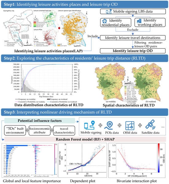
Figure 1. Research workflow.

2. Data and Methodology

2.1. Study Areas and Data

2.1.1. Study Areas

According to the Guangzhou Urban Master Plan (2017–2035), the main urban area of Guangzhou comprises the entirety of Liwan District, Yuexiu District, Tianhe District, and Haizhu District, as well as the area south of the North Second Ring Expressway in Baiyun District, the area south of Jiulong Town in Huangpu District, and the area north of the Guangming Expressway in Panyu District. To preserve the integrity of administrative divisions, seven districts, namely Liwan, Yuexiu, Tianhe, Haizhu, Baiyun, Huangpu, and Panyu, were designated as the research scope, with the specific boundaries illustrated in Figure 2. Moreover, to analyze the spatial differentiation characteristics of residents’ leisure travel distances at a micro scale, 500 m × 500 m grids were divided as the basic analytical units for this study [40,41,42], with the research area comprising a total of 8227 such grids.

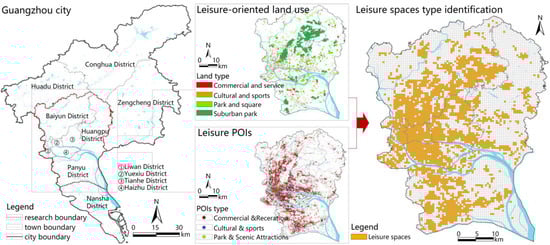
Figure 2. Study area and identifying leisure spaces.

2.1.2. Data Sources

The research integrates multiple data sources, primarily mobile phone signaling data and built environment data. Mobile phone signaling data was obtained from the Unicom Smart Footprint Platform, with data collection conducted in June 2021. It should be noted that mobile phone signaling data is not open-source. Acquiring such data requires payment of a fee to data service providers and is subject to a certain time lag. This dataset contains information such as dates, origin-destination (OD) points, travel types, and the number of China Unicom expanded users. To minimize the epidemic’s interference with analyzing the spatiotemporal pattern of residents’ leisure travel, this study selected 27 June (Sunday) and 30 June (Wednesday) as representative rest days and weekdays, respectively. By these dates, new COVID-19 infections had remained at zero for seven consecutive days. Python 3.9.0 software was used to process OD data related to residents’ living-leisure connections. Point of Interest (POI) data for 14 types of facilities within the study area in 2021 was acquired via the Gaode Map API interface (https://lbs.amap.com/api/webservice, accessed on 21 May 2021). Road network data was sourced from Open Street Map (http://download.geofabrik.de/asia.html, accessed on 21 May 2021). Moreover, the road network data within the study scope was extracted and processed for subsequent analysis. Building density data was derived from 2021 high-resolution satellite data with a spatial resolution of 10 m, from which building height and building base area data could be extracted. Data on large retail commercial outlets was obtained from the Development Plan of Key Commercial Functional Areas in Guangzhou (2020–2035) and supplemented by field surveys conducted in June 2021. Housing price data was collected by crawling 2021 second-hand housing prices from the Anjuke website (https://www.anjuke.com/, accessed on 21 May 2021) using Python web scraping tools.

2.2. Identifying Leisure-Based Trips

Drawing on the classification methods of leisure spaces in previous studies [43,44,45], this study categorizes leisure spaces into three types: commercial consumption, cultural and sports, and park sightseeing. Leisure spaces were identified by integrating land-use data and POI data, while leisure activities were identified by incorporating mobile phone signaling data, which reflects residents’ spatiotemporal activity patterns. Specifically, a grid was initially classified as a leisure space if leisure land comprised over 10% of its area or it had a high density of leisure facilities [45]. However, this classification was subsequently disqualified for grids encompassing major passenger flow hubs (e.g., airports, railway stations) or tertiary first-class hospitals. To be more specific, the screening method for grids with intensive leisure facility distribution involved three steps: first, excluding grids with zero leisure facilities; second, classifying the remaining spatial units into five grades based on facility quantity using the natural break point method; and finally, designating grade 2–5 units as grids with intensive leisure facility distribution (see Figure 2).

Subsequently, mobile phone signaling data was comprehensively utilized to further identify leisure activities. In this study, leisure activities are defined as a return journey between a residence and a leisure location. Therefore, it is crucial to identify the two types of spatial anchors: residential locations and leisure destinations. Specifically, a residential area was identified as the location where a user stayed for the longest duration during the observation period from 21:00 to 08:00, with such stays occurring on over 10 days within a month. Likewise, a workplace was determined as the location with the longest user stay during the 09:00–17:00 period, also with occurrences on more than 10 days monthly. For leisure venues, the identification followed a two-step logic. First, a non-commuting place was defined as a location where residents stayed for over 30 min in areas that are neither residential nor work-related [25,44]. Second, if such a non-commuting place fell within the leisure space units identified in the previous step, it was classified as a leisure venue. Through this approach, the raw signaling data was processed into OD data representing connections between residential areas and leisure venues. Moreover, the volume of leisure OD connections between grids was quantified, with a representative example of the data presented in Table 1.

Table 1. Residence-to-Leisure OD Data Sample.

Date	Origin_id	Destination_id	Origin_type	Destination_type	Trip_cnt
27 June 2021	10000	10782	Residential place	Leisure space	7
30 June 2021	10002	13912	Leisure space	Residence	14
30 June 2021	10010	10186	Residence	Leisure space	9

2.3. Variable and Nonlinear Model

2.3.1. Variable Description

In this study, the average RLTD within grids was used as the dependent variable. We measured RLTD as the Euclidean distance between an individual’s residence and their leisure destination [8,25]. A dataset of explanatory variables was constructed primarily based on built environment, supplemented with socioeconomic attribute variables and leisure travel characteristic variables. Drawing on relevant studies [28], built environment variables influencing leisure travel distance were operationalized using the five dimensions of “density”, “diversity”, “design”, “distance”, and “destination”, covering 16 indicators in total. Socioeconomic attribute variables, on the other hand, included three indicators: housing prices, age, and immigration proportion. As for leisure travel characteristic variables, they were represented by the leisure travel frequency indicator. In summary, this variable set consisted of 20 indicators in total, as detailed in Table 2.

Table 2. Model variable settings (Taking weekdays as an example).

Category	Name (Units)	Abbr.	Computational Method and Interpretation	Mean	Standard Deviation
Dependent variable
	Average leisure travel distance on weekday (km)	RLTD	Sum of weighted leisure travel distances divided by sum of weighted leisure travel frequencies at place of residence on weekday	9.476	4.756
Independent variable
Density	Residential population density (10,000 persons/km2)	POP	Population density per unit area within spatial units	1.482	1.923
Diversity	Mixed-use index of facilities *	DIV	Mixed-use status of 14 POI categories within spatial units, Mixed-use index = $-{\sum }_{i=1}^k{p}_{i}ln\left(p_i\right)$, where k denotes the number of POI classes within each spatial unit and $p_i$ denotes the proportion of class i POI counts	0.543	0.478
	Retail facilities density (1000 pcs/km2)	RFD	Number of retail facilities per unit area	0.085	0.144
	Catering service facilities density (1000 pcs /km2)	CFD	Number of catering service facilities per unit area	0.077	0.107
	Sports and recreation facilities density (1000 pcs/km2)	SRD	Number of sports and recreation facilities per unit area	0.004	0.009
	Educational and cultural facilities density (1000 pcs/km2)	ECD	Number of educational and cultural facilities per unit area	0.067	0.074
	Corporate facilities density (1000 pcs/km2)	CPD	Number of corporate facilities per unit area	2.139	1.594
Design	Road density (km/km2)	ROD	Total road length divided by the area of the spatial unit	0.186	0.124
	Building density (%)	BGD	Total building base area divided by total area	0.126	0.173
	Parking lot density (1000 pcs/km2)	PAD	Number of Parking lot facilities per unit area	1.618	1.501
Distance	Distance to the metro station (km)	DMS	Euclidean distance to the nearest Metro Station	3.685	3.324
	Bus Route Density (pcs/km2)	BRT	Number of bus route per unit area	17.323	23.433
Destination	CBD accessibility (km)	CBD	Euclidean distance to CBD (Huacheng Square)	14.995	7.213
	Large commercial complexes accessibility (km)	LCD	Euclidean distance to the nearest large commercial complexes	1.733	1.373
	Cultural and sports facilities accessibility (km)	CSD	Euclidean distance to the nearest cultural and sports facilities	0.940	0.775
	Park accessibility (km)	PA	Euclidean distance to the nearest park and square	0.848	0.601
Socioeconomic attributes	Housing price (10,000 yuan/m2)	HP	Average housing price within spatial units, derived using Kriging spatial interpolation	2.860	1.216
	Proportion of migrants (%)	MIG	Proportion of migrants within spatial units	0.353	0.139
	Age (%)	Age	Set values of 1, 2, 3, 4 and 5 for different age groups from youth to old age and calculate the weighted sum for the dummy variable of Age [25]	0.489	0.056
Travel characteristic	Leisure travel frequency (10,000 persons/km2)	LTF	Leisure travel frequency within spatial units	0.289	0.426

* The 14 types of POI facilities include shopping service, catering service, accommodation service, business residential, sports and leisure service, science-education-cultural service, daily life service, medical and healthcare service, government agencies and social organization, financial and insurance service, corporate enterprise, scenic spot, public facilities, and transportation service facilities.

2.3.2. Random Forest Model

The Random Forest (RF) model was employed to investigate the nonlinear effects of the built environment on leisure travel distance. As a machine learning model that integrates multiple decision tree classifiers, it uses the Bootstrap resampling method to randomly and repeatedly extract N training samples from the training set, which then serve as input for training M decision tree models. The final feature contribution result is determined by averaging the “voting” outcomes across different decision trees. Notably, compared with other machine learning models, RF exhibits advantages such as high robustness, strong generalization ability, and resistance to overfitting, thereby showing good adaptability to high-dimensional datasets [46]. Beyond this, when contrasted with traditional linear regression models, the RF model is particularly adept at handling complex nonlinear relationships between different types of data. This capability has led to its wide application in research on various topics, such as factors influencing residents’ destination choice, travel mode selection, and urban vitality [47]. Therefore, applying the RF model in this study can enhance the accuracy and reliability of analyzing the factors influencing the average leisure travel distance.

The random forest regression prediction model could be expressed as:

$$P\left(x\right)=\arg \underset{Y}{\max }{\sum }_{a=1}^{b}I[p_a\left(x\right)=Y]$$

(1)

In the formula, $P\left(x\right)$ denotes the combined classification model, $p_a$ represents a single decision tree classification model, x stands for the input sample, Y indicates the target variable, I [$p_a\left(x\right)=Y$] denotes the indicator function, a represents the sequence, and b denotes the number of iterations.

2.3.3. SHAP Model

This study leverages SHAP-based visualization to elucidate the results derived from the Random Forest model. To be specific, the SHAP model can provide insights such as the importance of characteristic variables, partial dependency diagrams of key variables, and characteristic interaction. Moreover, it has been widely applied in travel behavior research [48]. The SHAP interpreter is based on game theory, with its core being the evaluation of the marginal contribution of variables to the model prediction results by calculating the Shapley values of each sample. In this way, it reflects the global or local impact of variables on the prediction objectives. The average absolute Shapley value of a feature reflects the relative importance of the variable, which corresponds to the global impact on the model prediction results. In addition, the polarity of the Shapley value for a feature denotes whether its impact on the prediction constitutes a positive or negative contribution.

For a prediction sample X_i, its j-th feature is denoted as X_ij, with the Shapley value of X_ij being $f\left(X_{ij}\right)$, n represents the number of variables, the model prediction result of sample i is y_i, and the baseline prediction result (typically the average value of the target variables across all samples) is y_base. The formula is presented as follows:

$$y_i=y_{base}+f\left(X_{i1}\right)+f\left(X_{i2}\right)+f\left(X_{i3}\right)+...+f\left(X_{in}\right)$$

(2)

The Shapley value of a specific feature was determined by summing its contributions across all combinations of sample feature values, with the formula as follows:

$$f(X_{ij}) = {\sum }_{S\subseteq \left\{x_1,\dots ,x_n\right\}\backslash \left\{x_i\right\}}{\displaystyle \frac{\left|s\right|!(n-\left|s\right|-1)}{n!}}(val(s\cup \left\{x_i\right\})-val(S))$$

(3)

where S denotes a subset containing feature values, X represents the characteristic variable explaining the sample, n indicates the number of elements, and val(S) stands for the prediction of the feature values within set S.

3. Results

3.1. The Spatiotemporal Characteristics of Residents’ Leisure Travel Distance in Guangzhou

3.1.1. The Data Distribution Characteristics of Residents’ Leisure Travel Distance

First, an analysis of the curves plotting leisure travel distance against travel frequency revealed that as leisure travel distance increases, the number of residents engaging in such travel decreases significantly. This confirms that the frequency of leisure trips made by Guangzhou residents follows the distance decay law, as illustrated in Figure 3. In addition, residents’ leisure travel activities are more active on weekdays, with longer travel distances and stronger regularity compared to weekends. Specifically, the frequency of leisure travel doubles on weekdays compared to weekends. While both the mean and median leisure travel distances are higher on weekdays than on weekends, the standard deviation is lower, as shown in Table 3. Finally, with 5 km and 10 km as breakpoints, travel distance was divided into three intervals: short-distance travel (less than 5 km), medium-distance travel (5–10 km), and long-distance travel (more than 10 km). Statistics indicate that residents’ leisure travel activities in the study area are predominantly short- and medium-distance. Short-distance travel accounts for approximately half of the total leisure travel of residents, with a higher proportion of short-distance travel observed on weekends.

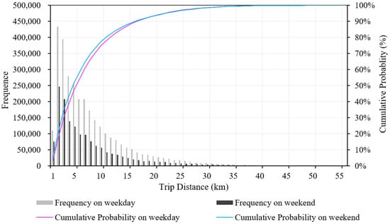
Figure 3. Frequency distribution of the leisure trip distances on weekday and weekend.

Table 3. Statistical Table of Leisure trip distances on weekday and weekend.

Period	Mean	Median	Standard Deviation	Proportion of Short Distance Trip (0–5 km)	Proportion of Longer Distance Trip (5–10 km)	Proportion of Long Distance Trip (10–15 km)
weekday	7.505	5.384	6.812	47%	28%	25%
weekend	7.085	4.716	6.909	52%	25%	23%

3.1.2. The Spatial Distribution Characteristics of Residents’ Leisure Travel Distance

This study first investigates whether residential leisure travel activities exhibit spatiotemporal heterogeneity. To this end, we aggregated residents’ leisure travel distances and frequencies into 500 m grids and calculated the average leisure travel distance from each grid, as illustrated in Figure 4. The analysis indicates that the distribution of the average leisure travel distance on weekdays and weekends exhibits certain spatial differences. To be more specific, on weekdays, the average leisure travel distance shows a concentric zonal pattern, with values increasing from the city center toward the periphery. Grids with an average leisure travel distance under 7 km constituted 31% of the total, concentrated in most areas of Tianhe District, Yuexiu District, Haizhu District, and Liwan District, as well as parts of southern Baiyun District and a few areas in central Panyu District. Conversely, several areas were identified as distinct high-value clusters for average leisure travel distance, with values exceeding 12 km: Zhongluotan Town in northern Baiyun District; Jiulong Town and Yonghe Street in northeastern Huangpu District; and Shilou Town in eastern Panyu District. In contrast, low-value areas of the average leisure travel distance on weekends exhibit salient polycentric agglomeration pattern. Grids with an average leisure travel distance under 7 km account for 45%, confirming that residents are more likely to engage in leisure activities within the vicinity of their homes [20].

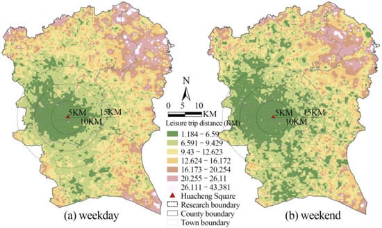
Figure 4. The spatial distribution characteristics of the average leisure travel distance.

3.2. Influencing Factors of the Average Leisure Travel Distance

3.2.1. Model Performance Comparison

Before formally constructing the model, to prevent multicollinearity among variables from interfering with model prediction results, the Pearson correlation coefficients of all variables were first examined. Specifically, variables with a correlation coefficient exceeding 0.8 were screened out. The results showed that high correlations existed between “education and cultural facilities density” and “parking lot density”, as well as between “sports and recreation facilities density” and “catering service facilities density”. Thus, only two indicators, namely “parking lot density” and “catering service facilities density”, were retained. Subsequently, to ensure no redundant independent variables were included, we evaluated multicollinearity using the variance inflation factor (VIF). We found that all variables had VIF values below 7.5, confirming the absence of severe collinearity. Furthermore, we used the fitting results of multiple models as a reference to select the optimal model for subsequent analysis. The alternative evaluated models included Random Forest Regression (RF), Extreme Gradient Boosting (XGBoost), Gradient Boosted Regression Trees (GBRT), Support Vector Machine (SVM), and Multiple Linear Regression (MLR). RMSE, MAE and R² were chosen as model evaluation indicators, where a lower RMSE, MAE and a higher R² indicate a better model fitting effect. As presented in Table 4, the RF model outperformed other models and more accurately predicted the average leisure travel distance. Specifically, compared to the MLR model, the RF model achieved lower error metrics, with RMSE reduced by 6% (weekday) and 3% (weekend), and MAE reduced by 6% and 3%, respectively. Corresponding improvements in R² were 10% and 8%. Furthermore, the RF model achieved lower RMSE and MAE than the XGBoost, GBRT, and SVM models, alongside consistently higher R² values.

Table 4. Results of multiple learning model fitting.

	RF	XGBoost	GBRT	SVM	MLR
RMSE (weekday)	2.977	3.072	3.076	3.775	3.17
MAE (weekday)	2.052	2.117	2.120	2.602	2.185
R2 (weekday)	0.601	0.575	0.574	0.358	0.547
RMSE (weekend)	3.869	3.983	4.024	4.739	3.982
MAE (weekend)	2.683	2.762	2.790	3.286	2.761
R2 (weekend)	0.477	0.447	0.435	0.217	0.447

In this study, the random forest model was implemented in Python 3.9.0, and the grid search cross-validation method was used to determine the optimal parameters. we evaluated the following parameters across a range of values: the number of decision trees (100, 200, 300, 400, 500), the maximum tree depth (None, 10, 20, 30), the minimum samples for node splitting (2, 5, 10), and the minimum samples for leaf nodes (1, 2, 4). Subsequently, the dataset, comprising 8227 samples, was split into training and test sets at an 8:2 ratio. A 5-fold cross-validation method was applied to the training process to prevent overfitting. Finally, after grid search, the model achieved the lowest RMSE, MAE and the highest R² with the following parameter combinations, as presented in Table 5.

Table 5. The optimal parameter set of the random forest prediction model.

	n_estimators	max_depth	min_sample_split	criterion
weekday	400	30	5	2
weekend	300	30	2	2

3.2.2. Feature Importance Analysis Based on SHAP

A random forest model and SHAP algorithm were employed to investigate the relationship between the average leisure travel distance and the built environment. Specifically, the relative importance of variables quantifies their capacity to minimize the loss function, while the average SHAP value of explanatory variables reflects their contribution to predicting the average leisure travel distance.

The relative importance of variables was calculated based on their SHAP mean absolute values, with the sum of relative importances across all explanatory variables set to 100%. The higher the SHAP value of an explanatory variable, the greater its contribution to the dependent variable (RLTD). To illustrate the distributional effects and direction of influence of variables’ average SHAP values, sampling points were jittered along the Y-axis. Each data point in the figure represents a sample, and its color denotes the magnitude of the corresponding feature value. Red samples indicate higher feature values, while blue samples indicate lower feature values. Moreover, the long-tailed distribution of these data points indicates that a small number of samples are significantly influenced by this feature (Figure 5).

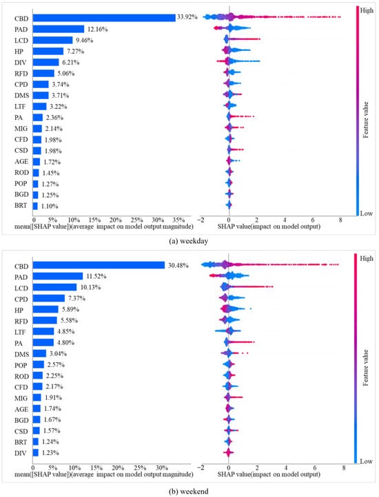
Figure 5. Relative importance of independent variables in different models.

For the weekday model, RLTD was most strongly associated with the distance to the Central Business District (CBD) (RI = 33.92%), parking facilities density (PAD) (RI = 12.16%), and the distance to large commercial districts (LCD) (RI = 9.46%). In addition, housing prices (HP), the mixed-use index of facilities (DIV), and retail facilities density (RFD) represent other strong predictors in this study. As the distance to CBD and the distance to large commercial districts increase, SHAP values also rise, indicating a significant positive correlation. Conversely, PAD, RFD, DIV, and HP exhibit negative correlations with leisure travel distance. For the weekend model, the rankings of relative importance of influencing factors differ slightly. While CBD, PAD, and LCD remain the top three strong predictors, the relative importance rankings of corporate and enterprise density (CPD), leisure travel frequency (LTF), distance to parks and squares (PA), residential population density (POP), and road density (ROD) have increased significantly. In contrast, the relative importance of DIV has decreased sharply.

3.2.3. Nonlinear Effects Based on SHAP

The SHAP explainable machine learning approach was employed to generate partial dependency plots for the random forest (RF) model, thereby analyzing nonlinear relationships between key explanatory variables and RLTD. The SHAP partial dependence plot depicts the relationship between a feature’s value (x-axis) and its impact on RLTD (y-axis). A positive SHAP value indicates a feature’s positive contribution to the model’s output, while a negative value signifies a negative contribution. Changes in the slope of the fitted curve indicate shifts in the strength of the feature’s influence. Consequently, all variables exhibit nonlinear relationships with the average leisure travel distance, with some variables displaying significant threshold effects (Figure 6).

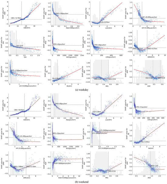
Figure 6. The partial dependence plots of key variables. The red line in the figure is the fitted curve between the feature value and its SHAP value, illustrating how each feature influences RLTD. Each blue dot denotes an individual sample.

For the weekday model, among built environment variables, CBD shows a positive correlation with RLTD. First, residential location significantly influences RLTD. Specifically, 20 km from the CBD represents a critical threshold—distances increase gradually from 0 to 20 km, however beyond this point, the growth rate accelerates substantially. Additionally, PA exhibits a positive correlation with RLTD: when the distance to parks is within 800 m, RLTD remains consistently short.

LCD and DMS both exhibit a “U”-shaped trend in their association on RLTD. For LCD, its relationship with RLTD shows a weak negative association when the distance is less than 2 km, which shifts to a significant positive association when the distance exceeds 2 km. Similarly, the association between DMS and RLTD follows a three-phase pattern: a suppressive association from 0 to 1 km, a plateau between 1 and 3 km, and a strengthening positive association beyond 3 km. These patterns suggest that proximity to subway stations is a strong predictor and may serve as a key mechanism through which enhanced transit accessibility broadens the spatial scope of RLTD.

PAD, DIV, RFD, and CPD all exhibit significant threshold effects. PAD exerts a triphasic inhibitory effect on leisure travel distance, transitioning from a rapid decline (PAD < 50 units/km²) to a negligible effect (50–200 units/km²) and finally to a slow decrease (>200 units/km²). Similarly, DIV, RFD, and CPD display similar threshold trends, with their respective thresholds being 0.47, 42 pcs/km², and 44 pcs/km².

In terms of socioeconomic attributes, HP exhibits a significant threshold effect: rising prices suppress leisure travel distance from residential areas below 26,000 yuan/m², after which the effect plateaus. Furthermore, the impacts of migration status (MIG) and age (AGE) on leisure travel distance display a weak U-shaped pattern. This nonlinear pattern suggests distinct leisure travel preferences between local residents and migrants, as well as across different age groups. Additionally, the predictive association between LTF and RLTD shows a significant threshold, identified at 1700 persons/km².

Compared with the weekday model, the weekend model exhibits a broadly consistent direction of association for most explanatory variables on RLTD, although with notable differences in their threshold values. For built environment variables, the threshold for CBD increases to 25 km, whereas the thresholds for LCD and PA rise to 2.6 km and 1.07 km, respectively. Moreover, the thresholds for PAD, CPD, and RFD decrease to 80 pcs/km², 31 pcs/km², and 22 pcs/km², respectively. Notably, population density (POP) exhibits a distinct threshold pattern: RLTD shows a sharp positive association with density below 5600 persons/km², beyond which the relationship levels off. In terms of socioeconomic attributes, the associations of HP and MIG on weekends show little change compared with those on weekdays.

AGE demonstrates a negative correlation with leisure travel distance, exhibiting a distinct threshold effect at 1.42. Conversely, LTF and leisure travel distance share an inverted U-shaped relationship, manifesting as an initial upswing to a low peak at 300 persons/km², succeeded by a gentle downturn.

3.2.4. Interaction Effects Based on SHAP

Further exploration of the combined effects of key explanatory variables and their strongly interactive variables on the average leisure travel distance is shown in Figure 7. A SHAP interaction plot displays the SHAP interaction value (y-axis) against the primary feature’s value (x-axis), with point color indicating the interacting feature’s value. Distinct color stratification, such as red points above and blue points below the fitted curve, reveals a strong interaction between the features.

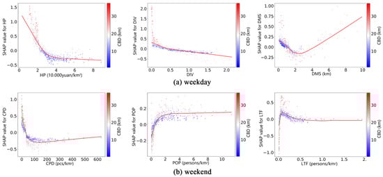
Figure 7. Interaction effect plots of partial key variables. The red line is the fitted curve between the values of the two interacting variables and their SHAP values, characterizing the combined effect of the two interacting variables on RLTD. Each dot denotes an individual sample.

In the weekday model, HP, DIV, and DMS, respectively, show notable interactive associations with CBD. First, the interaction between HP and CBD indicates that when HP is within 20,000 yuan/m², greater distance to the CBD is associated with significantly increased RLTD. Conversely, the interaction between DIV and CBD shows that when DIV is below 0.47 and CBD exceeds 20 km, lower DIV values are associated with higher RLTD. Third, the interaction between DMS and CBD indicates that when the distance to metro station is within 2 km, a lower CBD are associated with reduced RLTD. It suggests that residents in peripheral areas rely more on metro accessibility within 2 km for leisure activities.

In the weekend model, interaction effects among HP, DIV, DMS, and CBD persist, while additional interactions are observed between CPD, POP, LTF, and CBD. In particular, the interaction between CPD and CBD indicates that when CPD is within 31 units/km², it is associated with lower RLTD in both peripheral and central urban areas, with a more pronounced association in peripheral areas. It can be inferred that higher enterprise density in peripheral areas may have a stronger marginal association with reduced RLTD. The interactions of POP and LTF with CBD reveal a distinct pattern in peripheral areas. Specifically, when POP falls below 5600 persons/km² or LTF under 300 persons/km², these lower densities are associated with a more noticeable decrease in RLTD.

4. Discussion

This study clarifies the spatiotemporal characteristics of RLTD in megacities and systematically investigates the nonlinear impacts of the built environment on RLTD. As such, these findings have significant implications for reducing residents’ leisure travel costs and improving their leisure travel experiences [49]. Two key findings are summarized as follows:

First, this study proposes a refined identification method for urban leisure travel behavior that integrates multi-source data, which more accurately reveals residents’ leisure travel characteristics. For one thing, compared with the identification method for generalized leisure travel (i.e., travel behavior with third places as destinations), this study explicitly defines leisure activities as three main types. For another, the travel distance measurement method integrating multi-source data can effectively address the sample bias caused by the use of a single data source in existing studies.

Using this method, this study finds that leisure activities of Guangzhou residents are dominated by short-to-medium-distance travel, exhibiting strong spatiotemporal heterogeneity. This aligns with the insight that the pandemic reshaped residents’ spatiotemporal behaviors [50]. Specifically, residents’ activities were affected by the pandemic prevention and control policy of “no unnecessary travel.” On weekends, greater freedom and heightened risk aversion increased the preference for nearby leisure, shortening travel distances. By contrast, on weekdays, however, leisure activities often appended to necessary trips like commuting, expanding their spatial range and increasing travel distance. These findings highlight the need to account for spatiotemporal differences in leisure activities, placing equal emphasis on both weekday and weekend patterns. It also underscores the value of studying leisure activities occurring outside residential areas, such as near workplaces or other activity hubs.

Additionally, RLTD show distinct spatiotemporal patterns: on weekdays, they form a circular distribution, increasing from the central urban area to peripheral regions; on weekends, they exhibit a clear multi-center agglomeration. This mirrors conclusions from relevant studies [20]. As the greater spatiotemporal freedom on weekends, combined with the decentralized distribution of leisure facilities in megacities, promotes nearby and multi-destination leisure travel.

Second, built environment variables exert significant nonlinear impacts and threshold effects on RLTD, with these impacts varying between weekdays and weekends. This finding breaks from existing studies that focus solely on linear relationships, emphasizing the importance of exploring nonlinear dynamics.

To elaborate, three key observations emerge. For one, residential location, transportation facility accessibility, and proximity to large commercial centers show the highest predictive importance for RLTD. Beyond that, on weekdays, variables such as HP, DIV, and RFD also demonstrate notable associations with RLTD. Although prior work emphasizes CBD and DIV [39,51], we show that PAD is equally significant. Specifically, improving destination accessibility, particularly through better “last-mile” connections, facilitates short-to-medium leisure trips. Such improvements offer new evidence linking accessibility to travel behavior. High SHAP values for LCD and RFD underscore shopping-related activities as a priority in residents’ leisure activity choices during the pandemic. Meanwhile, the right-tailed SHAP distribution for DIV indicates that limited urban functional diversity near residences is associated with longer leisure travel distance. Subway accessibility (DMS) also outperforms bus route density (BRT) in predicting travel distance, reflecting a stronger association between metro access and residents’ leisure travel. Therefore, metro accessibility around residences may serve as a key factor in supporting residents’ leisure mobility. On weekends, by contrast, DIV shows reduced predictive importance, while variables such as CPD, LTF, PA, POP, and ROD gain significance. The predictive power of CPD on weekends aligns with Tao et al.’s findings [52], likely because corporate agglomeration enhances functional mixing and transportation options, making nearby leisure more accessible. PA’s prominence, meanwhile, suggests residents are willing to travel farther for park recreation on weekends. This may stem from their desire to seek “restorative experiences” amid natural landscapes, which helps alleviate urban stress.

Another key point is that three variables, namely CBD, PAD, and LCD, exert nonlinear impacts on leisure travel distance expansion. On weekdays, CBD shows a positive correlation with travel distance, with a critical threshold at 20 km: beyond this, distance increases rapidly. This aligns with existing studies [39,53]. As urban leisure facilities are predominantly concentrated in the city center, residents far from the CBD must travel farther for leisure. These findings reveal significant spatial inequity in leisure travel between residents in Guangzhou’s urban core and peripheral areas, providing critical evidence on the limited efficacy of its polycentric structure. The current polycentric system has failed to effectively alleviate long-distance leisure travel pressure generated by the urban core. Thus, urban planning practice should prioritize developing a more balanced polycentric spatial structure and promoting equitable distribution of urban facilities to enhance spatial coordination and social equity. PAD shows a threshold effect: adequate parking near residences is associated with reduced travel distance, but beyond a certain point, additional parking shows diminishing returns. LCD follows a “U-shaped” trend: distances decrease when commercial facilities are within 2 km but increase beyond this range, emphasizing the importance of balanced commercial-residential layouts. On weekends, thresholds for CBD, LCD, and PA rise, while those for PAD, CPD, and RFD fall. This suggests that residents exhibit diverse destination choices on weekends, potentially reflecting greater flexibility in their time budgets.

Finally, interaction analyses reveal that residential location, when combined with variables like local housing prices, land-use mix, or subway accessibility, is associated with significantly increased leisure travel distance. This addresses the limitation of single-factor analysis in existing studies. In conclusion, these findings challenge the simplistic positive/negative assumptions regarding environmental variables in previous studies [23] by demonstrating their dual role. While these variables are associated with facilitated leisure travel within specific thresholds, their predictive strength often weakens beyond these ranges. This nuanced understanding provides a fresh perspective on person-environment interactions and supports the design of more effective planning interventions.

Based on the above findings, this study proposes corresponding policy implications as follows: To start with, regional accessibility should be prioritized. It is recommended to promote a more balanced polycentric urban structure, and focus on optimizing the layout of leisure facilities and transportation accessibility in urban peripheral regions (over 20 km away from the center) [37]. Meanwhile, efforts should be made to achieve a coordinated layout and functional integration between residential clusters and key commercial districts. By implementing elastic land-use policies that allow residential land to accommodate a certain proportion of commercial land, functional mixing can be enhanced, thereby increasing the share of residents who engage in leisure activities nearby.

Next, policymakers are advised to refer to the most effective ranges of specific variables and formulate targeted intervention measures to reduce extremely long-distance leisure travel among residents. For example, a differentiated parking facility supply strategy should be adopted: priority should be given to increasing supply in built-up areas with insufficient parking density (less than 50 pcs/km²), while over-construction in high-density areas should be avoided. Furthermore, optimizing the layout of commercial facilities within a 2 km radius of residential areas is an effective way to reduce long-distance leisure travel. This finding also serves as a key consideration for Guangzhou in building an “International Consumption Center City.”

In addition, efforts should be made to avoid negative externalities caused by the monofunctional residential clusters that are isolated from other amenities in urban fringe areas. One approach is to promote the organic integration of residential units at different price levels, creating diverse and inclusive residential environments. This ensures that residential areas with varying price ranges can share high-quality leisure facility services. For instance, in urban fringe residential areas with extremely low functional mix, targeted efforts are needed to make up for deficiencies in facilities such as shopping centers, park squares, and corporate establishments. Furthermore, subway station accessibility should be enhanced by improving the network and shared bicycle layout, alongside promoting TOD-guided development around stations. These combined measures can effectively reduce unnecessary long-distance leisure travel by residents.

Despite providing valuable findings and recommendations, this study has certain limitations that warrant further exploration. First, it only examines the impact of the built environment around residential areas. Existing research has shown that the built environment around residential and workplace locations have distinct influences on travel characteristics [33]. Therefore, future studies should comprehensively investigate how the built environments around these two types of locations differ in their effects on leisure travel distance. Second, this study does not consider the influence of different transportation modes (e.g., bus, subway, private car, or combined modes). Notably, the impact of the built environment on residents’ travel distance varies across transportation modes [14]. To gain more detailed insights, future research will integrate transportation survey data to analyze differences in variable impacts across various modes. Finally, despite its strengths in capturing complex patterns, the machine learning approach has inherent limitations in addressing urban social-science questions. Therefore, our findings warrant further grounded verification through complementary methods such as survey questionnaires.

5. Conclusions

This study leverages multi-source data to identify residents’ leisure travel behavior and reveals the spatiotemporal patterns of RLTD in Guangzhou. It further employs random forest models to investigate the nonlinear relationships between built environment attributes and RLTD. The key findings are summarized as follows: (1) Leisure travel activities of Guangzhou residents are dominated by short-to-medium-distance trips, with significant spatiotemporal variability in travel distance distributions. Specifically, on weekdays, travel distances exhibit a regional circular distribution pattern, where distances increase progressively from the central urban area to peripheral regions. On weekends, by contrast, a distinct multi-center agglomeration pattern emerges. (2) Whether on weekdays or weekends, proximity to central business districts (CBD) and large commercial centers, alongside the rational allocation of parking facilities, emerges as the most influential predictor of RLTD. However, the predictive importance of commercial diversity and corporate spatial layout varies significantly across temporal contexts. (3) Built environment variables exert nonlinear effects on RLTD. Notably, certain variables, including housing prices, mixed-use index of facilities, and shopping facility density, show meaningful associations with RLTD only within specific threshold ranges. In addition, the “distance to CBD” variable demonstrates distinct interactive associations with other built environment attributes in predicting travel distance.

References

- Iso-Ahola, S.E. Basic dimensions of definitions of leisure. J. Leis. Res. 1979, 11, 28–39. [Google Scholar] [CrossRef]
- Newman, D.B.; Tay, L.; Diener, E. Leisure and Subjective Well-Being: A Model of Psychological Mechanisms as Mediating Factors. J. Happiness Stud. 2013, 15, 555–578. [Google Scholar] [CrossRef]
- Sallis, J.F.; Cerin, E.; Conway, T.L.; Adams, M.A.; Frank, L.D.; Pratt, M.; Salvo, D.; Schipperijn, J.; Smith, G.; Cain, K.L.; et al. Physical activity in relation to urban environments in 14 cities worldwide: A cross-sectional study. Lancet 2016, 387, 2207–2217. [Google Scholar] [CrossRef] [PubMed]
- Lloyd, K.; Auld, C. Leisure, public space and quality of life in the urban environment. Urban Policy Res. 2003, 21, 339–356. [Google Scholar] [CrossRef]
- Peter, H.; Michael, A. Positive moods derived from leisure and their relationship to happiness and personality. Personal. Individ. Differ. 1998, 25, 523–535. [Google Scholar]
- Chen, Y.; Wang, B.; Huang, J.; Gao, H.; Shu, X. Urban Physical Environments Promoting Active Leisure Travel: An Empirical Study Using Crowdsourced GPS Tracks and Geographic Big Data from Multiple Sources. Land 2024, 13, 589. [Google Scholar] [CrossRef]
- Chica-Olmo, J.; Lizárraga, C. Effect of Interaction between Distance and Travel Times on Travel Mode Choice when Escorting Children to and from School. J. Urban Plan. Dev. 2022, 148, 05021055. [Google Scholar] [CrossRef]
- Li, X.; Xu, J.; Du, M.; Liu, D.; Kwan, M.-P. Understanding the spatiotemporal variation of ride-hailing orders under different travel distances. Travel Behav. Soc. 2023, 32, 100581. [Google Scholar] [CrossRef]
- Hartieni, P.; Joewono, T.B.; Dharmowijoyo, D. The effects of planned behaviour, spatiotemporal variables and lifestyle on public transport use: An exploratory study. Transp. Res. Part A Policy Pract. 2024, 190, 104255. [Google Scholar] [CrossRef]
- Jiang, Y.; Qin, J.; Wu, T. Understanding the spatiotemporal response of dockless bike-sharing travel behavior to the small outbreaks of COVID-19. Appl. Geogr. 2025, 175, 103488. [Google Scholar] [CrossRef]
- Lin, J.J.; Yu, T.P. Built environment effects on leisure travel for children: Trip generation and travel mode. Transp. Policy 2011, 18, 246–258. [Google Scholar] [CrossRef]
- Lin, L. Leisure-time physical activity, objective urban neighborhood built environment, and overweight and obesity of Chinese school-age children. J. Transp. Health 2018, 10, 322–333. [Google Scholar] [CrossRef]
- Gul, Y.; Sultan, Z.; Moeinaddini, M.; Jokhio, G.A. The effects of physical activity facilities on vigorous physical activity in gated and non-gated neighborhoods. Land Use Policy 2018, 77, 155–162. [Google Scholar] [CrossRef]
- Long, Y.; Ao, Y.B.; Li, H.M.; Bahmani, H.; Li, M.Y. Non-linear effects of children’s daily travel distance on their travel mode choice considering different destinations. J. Transp. Geogr. 2024, 118, 103921. [Google Scholar] [CrossRef]
- Zhao, X.K.; Huang, H.; Lin, G.S.; Lu, Y.X. Exploring temporal and spatial patterns and nonlinear driving mechanism of park perceptions: A multi-source big data study. Sustain. Cities Soc. 2025, 119, 106083. [Google Scholar] [CrossRef]
- Xi, Y.F.; Hou, Q.H.; Duan, Y.Q.; Lei, K.X.; Wu, Y.; Cheng, Q.Y. Exploring the Spatiotemporal Effects of the Built Environment on the Nonlinear Impacts of Metro Ridership: Evidence from Xi’an, China. ISPRS Int. J. Geo-Inf. 2024, 13, 105. [Google Scholar] [CrossRef]
- Toger, M.; Türk, U.; Östh, J.; Kourtit, K.; Nijkamp, P. Inequality in leisure mobility: An analysis of activity space segregation spectra in the Stockholm conurbation. J. Transp. Geogr. 2023, 111, 103638. [Google Scholar] [CrossRef]
- He, S.; Yu, S.; Wei, P.; Fang, C. A spatial design network analysis of street networks and the locations of leisure entertainment activities: A case study of Wuhan, China. Sustain. Cities Soc. 2019, 44, 880–887. [Google Scholar] [CrossRef]
- Liu, J.; Meng, B.; Shi, C.S. A multi-activity view of intra-urban travel networks: A case study of Beijing. Cities 2023, 143, 104634. [Google Scholar] [CrossRef]
- Xue, D.; Xinmeng, C.; Xin, Y.; Yongyong, S. Residents’ Leisure and entertainment Travel Preference and Urban Residential-Leisure Function Pattern: A Case Study of Xi’an. Geogr. Geo-Inf. Sci. 2024, 40, 71–79+121. [Google Scholar] [CrossRef]
- Liu, Y.; Zhang, Y.; Jin, S.T.; Liu, Y. Spatial pattern of leisure activities among residents in Beijing, China: Exploring the impacts of urban environment. Sustain. Cities Soc. 2020, 52, 101806. [Google Scholar] [CrossRef]
- Shan, Z.R.; Jin, L.L.; Yuan, M.; Zhang, X.Y.; Huang, Y.P. Research on Influencing Factors and Optimization Strategies of Travel Distance for Workplace-originated Shopping Trips: Taking Wuhan City as an Example. Areal Res. Dev. 2024, 43, 71–77. [Google Scholar] [CrossRef]
- Qi, L.L.; Zhou, S.H. The Influence of Neighborhood Built Environments on the Spatial-temporal Characteristics of Residents’ Daily Leisure Activities: A Case Study of Guangzhou. Sci. Geogr. Sin. 2018, 38, 31–40. [Google Scholar] [CrossRef]
- Cao, Y.; Wang, L.X.; Wu, H.; Yan, S.Q.; Shen, S.W. Identification and Mechanism of Residents’ Regional Non-Commuting Flow Patterns Based on the Gradient Boosting Decision Tree Model: A Case Study of the Shanghai Metropolitan Area. Land 2023, 12, 1652. [Google Scholar] [CrossRef]
- Chen, L.K.; Chen, M.X.; Fan, C. Age disparities and socioeconomic factors for commuting distance in Beijing by explainable machine learning. Cities 2024, 155, 105493. [Google Scholar] [CrossRef]
- Zheng, Y.; Deng, A.X.; Yin, Z.J.; Li, W.Q. Assessing travelers’ preferences for online bus-hailing service across various travel distances: Insights from Chinese metropolitan areas. Transp. Res. Part A Policy Pract. 2024, 187, 104159. [Google Scholar] [CrossRef]
- Aghaabbasi, M.; Chalermpong, S. Machine learning techniques for evaluating the nonlinear link between built-environment characteristics and travel behaviors: A systematic review. Travel Behav. Soc. 2023, 33, 100640. [Google Scholar] [CrossRef]
- Duan, Z.Y.; Zhao, H.R.; Li, Z.M. Non-linear effects of built environment and socio-demographics on activity space. J. Transp. Geogr. 2023, 111, 103671. [Google Scholar] [CrossRef]
- Liu, J.X.; Wang, B.; Xiao, L.Z. Non-linear associations between built environment and active travel for working and shopping: An extreme gradient boosting approach. J. Transp. Geogr. 2021, 92, 103034. [Google Scholar] [CrossRef]
- Tao, T.; Wang, J.Y.; Cao, X.Y. Exploring the non-linear associations between spatial attributes and walking distance to transit. J. Transp. Geogr. 2020, 82, 102560. [Google Scholar] [CrossRef]
- Liu, Y.; Li, Y.P.; Yang, W.; Hu, J. Exploring nonlinear effects of built environment on jogging behavior using random forest. Appl. Geogr. 2023, 156, 102990. [Google Scholar] [CrossRef]
- Peng, Y.A.; Yang, L.C. Effect of the Community-level Built Environment on Cycling Behavior from the Perspective of Differences in Trip Purposes. South Archit. 2025, 4, 100–107. [Google Scholar] [CrossRef]
- Xiong, Q.Q.; Xing, L.J.; Wang, L.Y.; Liu, Y.F.; Liu, Y.L. Comparing the impacts of built environment across different objective life neighborhoods on the out-of-home leisure activities of employed people using massive mobile phone data. Appl. Geogr. 2024, 171, 103382. [Google Scholar] [CrossRef]
- Bai, X.H.; Zhou, M.; Li, W.M. Analysis of the influencing factors of vitality and built environment of shopping centers based on mobile-phone signaling data. PLoS ONE 2024, 19, e0296261. [Google Scholar] [CrossRef]
- Ding, C.; Cao, X.Y.; Næss, P. Applying gradient boosting decision trees to examine non-linear effects of the built environment on driving distance in Oslo. Transp. Res. Part A Policy Pract. 2018, 110, 107–117. [Google Scholar] [CrossRef]
- Cheng, L.; Chen, X.W.; De Vos, J.; Lai, X.J.; Witlox, F. Applying a random forest method approach to model travel mode choice behavior. Travel Behav. Soc. 2019, 14, 1–10. [Google Scholar] [CrossRef]
- Guo, C.; Jiang, Y.Q.; Qiao, R.L.; Zhao, J.B.; Weng, J.C.; Chen, Y. The nonlinear relationship between the active travel behavior of older adults and built environments: A comparison between an inner-city area and a suburban area. Sustain. Cities Soc. 2023, 99, 104961. [Google Scholar] [CrossRef]
- Yin, C.; Liu, J.H.; Sun, B.D. Effects of built and natural environments on leisure physical activity in residential and workplace neighborhoods. Health Place 2023, 81, 103018. [Google Scholar] [CrossRef]
- Liu, Y.; He, D.L.; Lei, J.Y.; He, M.W.; Shi, Z.B. Investigating the non-linear influence of the built environment on passengers’ travel distance within metro and bus networks using smart card data. Multimodal Transp. 2025, 4, 100188. [Google Scholar] [CrossRef]
- Li, J.; Zhao, P.J.; Zhang, M.Z.; Deng, Y.L.; Liu, Q.Y.; Cui, Y.Z.; Gong, Z.Y.; Liu, J.; Tan, W.C. Exploring collective activity space and its spatial heterogeneity using mobile phone signaling Data: A case of Shenzhen, China. Travel Behav. Soc. 2025, 38, 100920. [Google Scholar] [CrossRef]
- Guan, C.H.; Zhou, Y.C. Exploring environmental equity and visitation disparities in peri-urban parks: A mobile phone data-driven analysis in Tokyo. Landsc. Urban Plan. 2024, 248, 105104. [Google Scholar] [CrossRef]
- Gao, X.; Wang, H.; Liu, L. Profiling Residents’ Mobility with Grid-Aggregated Mobile Phone Trace Data Using Chengdu as the Case. Sustainability 2021, 13, 13713. [Google Scholar] [CrossRef]
- Liu, S.; Long, Y.; Zhang, L.; Liu, H. Quantifying and Characterizing Urban Leisure Activities by Merging Multiple Sensing Big Data: A Case Study of Nanjing, China. Land 2021, 10, 1214. [Google Scholar] [CrossRef]
- Zhang, X.; Rui, J.; Xia, G.; Yang, J.; Cai, C.; Zhao, W. Revealing disparities and driving factors in leisure activity segregation of residents and tourists: A data-driven analysis of smart phone data. Appl. Geogr. 2025, 176, 103513. [Google Scholar] [CrossRef]
- Wang, Y. Research on Spatio-Temporal Characteristic and Influencing Factors of Residents’ Leisure Activities Based on Multisource Big Data—Take Nanjing as an Example. Master’s Thesis, Southeast University, Nanjing, China, 2021. [Google Scholar]
- Rodriguez Galiano, V.; Sanchez Castillo, M.; Chica Olmo, M.; Chica Rivas, M. Machine learning predictive models for mineral prospectivity: An evaluation of neural networks, random forest, regression trees and support vector machines. Ore Geol. Rev. 2015, 71, 804–818. [Google Scholar] [CrossRef]
- Zhou, W.; Liang, Z.; Fan, Z.; Li, Z. Spatio–temporal effects of built environment on running activity based on a random forest approach in Nanjing, China. Health Place 2024, 85, 103176. [Google Scholar] [CrossRef]
- Yang, X.P.; Li, J.Y.; Fang, Z.X.; Chen, H.F.; Li, J.Y.; Zhao, Z.Y. Influence of residential built environment on human mobility in Xining: A mobile phone data perspective. Travel Behav. Soc. 2024, 34, 100665. [Google Scholar] [CrossRef]
- Lin, Y.X.; Liu, Y. Let the city heal you: Environment and activity’s distinct roles in leisure restoration and satisfaction. Cities 2024, 154, 105336. [Google Scholar] [CrossRef]
- Lee, S.; Ko, E.; Jang, K.; Kim, S. Understanding individual-level travel behavior changes due to COVID-19: Trip frequency, trip regularity, and trip distance. Cities 2023, 135, 104223. [Google Scholar] [CrossRef]
- Shao, Q.; Zhang, W.; Cao, X.; Yang, J.; Yin, J. Threshold and moderating effects of land use on metro ridership in Shenzhen: Implications for TOD planning. J. Transp. Geogr. 2020, 89, 102878. [Google Scholar] [CrossRef]
- Tao, T.; Cao, J. Exploring nonlinear and collective influences of regional and local built environment characteristics on travel distances by mode. J. Transp. Geogr. 2023, 109, 103599. [Google Scholar] [CrossRef]
- Ding, C.; Mishra, S.; Lu, G.Q.; Yang, J.W.; Liu, C. Influences of built environment characteristics and individual factors on commuting distance: A multilevel mixture hazard modeling approach. Transp. Res. Part D Transp. Environ. 2017, 51, 314–325. [Google Scholar] [CrossRef]
Disclaimer/Publisher’s Note: The statements, opinions and data contained in all publications are solely those of the individual author(s) and contributor(s) and not of MDPI and/or the editor(s). MDPI and/or the editor(s) disclaim responsibility for any injury to people or property resulting from any ideas, methods, instructions or products referred to in the content. |
© 2025 by the authors. Licensee MDPI, Basel, Switzerland. This article is an open access article distributed under the terms and conditions of the Creative Commons Attribution (CC BY) license (https://creativecommons.org/licenses/by/4.0/).