Article

Multi-Scenario Simulating the Impacts of Land Use Changes on Ecosystem Health in Urban Agglomerations on the Northern Slope of the Tianshan Mountain, China

1
School of Public Administration, Hohai University, Nanjing 211000, China
2
Engineering Research Center of Ministry of Education for Mine Ecological Restoration, China University of Mining and Technology, Xuzhou 221000, China
*
Author to whom correspondence should be addressed.
Land 2024, 13(5), 571; https://doi.org/10.3390/land13050571
Submission received: 25 March 2024 / Revised: 16 April 2024 / Accepted: 23 April 2024 / Published: 25 April 2024

Abstract

:
It is of great significance for scientific land use planning and ecological security protection to clarify the impacts of land use changes on an ecosystem’s health. Based on the dynamic evolution of land use and ecosystem health on the Northern Slope of Tianshan Mountain (NSTM) from 2000 to 2020, this study utilized the patch-generating land use simulation (PLUS) model, the Vitality–Organization–Resilience–Services (VORS) model, and the elasticity approach to assess the impacts of land use changes on ecosystem health under four different scenarios: Natural Development Scenario (ND), Farmland Conservation Priority Scenario (FP), Ecological Conservation Priority Scenario (EP), and Urban Development Priority Scenario (UD). The results indicate that (1) land use on the NSTM from 2000 to 2020 was predominantly characterized by barren land and grassland. (2) The overall level of ecosystem health on the NSTM was poor from 2000 to 2020 but showed a gradual improvement trend. (3) Ecosystem health levels vary greatly across scenarios. In general, ecosystem health improves under FP and EP scenarios but deteriorates significantly under ND and UD scenarios. The resilience of ecosystem health varies significantly across different land categories. In the future, optimizing the current land use pattern and refining the ecological protection policy are essential to enhance ecosystem health and services in the NSTM.

1. Introduction

The natural ecosystem offers essential resources and services crucial for human survival and advancement [1,2]. Preserving ecosystem health (EH) is vital for addressing global climate change and attaining sustainable socioeconomic progress [3]. Nevertheless, the escalating global population and rapid urbanization and industrialization have placed unprecedented pressure on the ecosystems that sustain human life. Ecological concerns, including land degradation and a marked decline in biodiversity, are gaining increasing prominence. Over the past century, human activities have profoundly transformed global land use and coverage, representing a fundamental facet of global ecological change [4] and a significant means through which human actions influence ecosystems [5]. This transformation influences regional climate [6], hydrology [7], and biodiversity [8], consequently impacting the quality and service levels of ecosystems [9]. Global ecosystems are in the face of unprecedented population growth and the impact of human activities [10,11]. Hence, elucidating the effects of land use changes on EH and forecasting future trends holds immense importance in optimizing regional ecological management and territorial spatial planning, as well as fostering harmonious coexistence between humans and nature.
A robust ecosystem possesses the capacity to sustain the stability and continuity of its organization, structure, and function [12], as well as demonstrating adaptive self-regulation and resilience in recovering from external disruptions [13]. Recently, scholars both domestically and internationally have conducted comprehensive research on the effects of land use changes on ecosystem services [14], ecological vulnerability [15], biodiversity [16,17], and particularly EH [5]. This focus on EH underscores its pivotal role in the assessment and governance of ecosystems [2]. Approaches for ecosystem health assessment (EHA) encompass the indicator species method and the indicator system method. The indicator species method entails community assessments or toxicological studies on specific species indicative of EH. Nevertheless, this method presents certain challenges, including ambiguous selection criteria for indicator species, biased evaluation outcomes [18], and limited applicability [19]. The indicator system method is commonly employed in ecological health assessment due to its capacity to mitigate the aforementioned constraints. This method encompasses the integrated indicator model and the ambiguous–comprehensive evaluation model [19]. The widely utilized Vitality–Organization–Resilience (VOR) framework [20] serves as a cornerstone for developing indicator systems. Furthermore, the ongoing exploration of the Vitality–Organization–Resilience–Services (VORS) model, incorporating ecosystem service valuation, aims to account for the influences of regional scales [19] and spatial mosaics [2] on EHA. Past studies have examined how EH responds to changes in land use across diverse scales, regions, and viewpoints [5,21,22,23], culminating in a consensus that land use changes predominantly impact EH. Efforts have been undertaken to forecast future ecological health amidst land use changes by employing multi-model coupling and scenario analyses [24], aiming to capture the complex interplay between ecosystems and human activities [25,26]. Currently, simulation models for predicting land use are widely used, including the Conversion of Land Use and its Effects at Small regional extent (CLUE-S) model [27], the Future Land Use Simulation (FLUS) model [28], the Patch-generating Land Use Simulation (PLUS) model [29] and others. Scenario analysis involves applying distinct natural, economic, and social development scenarios to a specific land use prediction model, unveiling the land use alterations and their implications for EH across various developmental contexts. For instance, Pan et al. [21] predicted the joint impacts of future climate and land use changes on EH under different Representative Concentration Pathway (RCP) scenarios based on the FLUS model. Liang et al. [30] developed the PLUS model for predicting future sustainable land use scenarios by combining cellular automata (CA) with land expansion analysis strategies, effectively improving the simulation accuracy and credibility of traditional CA models. Li et al. [26] used the IBIS and VORS models to measure EH level and its spatiotemporal features under different land use scenarios in the future. Considering that 40% of the world’s land is situated in arid and semi-arid zones, the ecosystem in these areas is notably delicate and responsive. Human-induced land use changes can easily impact the ecological and environmental conditions within the region. Establishing a sustainable equilibrium between EH and land use poses a considerable challenge for arid and semi-arid regions striving for high-quality development. However, there remains an insufficiency in modelling scenarios and predicting the impact of land use change on EH within these zones. This limitation significantly constrains the implementation of construction and development planning, as well as the enforcement of ecological and environmental conservation measures within the region.
Located in the heart of Asia, the urban agglomeration on the northern slope of the Tianshan Mountain (NSTM) boasts a distinctive continental arid climate and a delicate ecological system [31]. Situated as the sole frontier urban agglomeration in northwestern China, the NSTM lies proximate to the oil- and gas-endowed Central Asian region, brimming with mineral wealth, thus serving as a vital strategic hub for China’s energy development. The implementation of strategies such as the “One Belt, One Road” and the “Western development” have converged to foster the enduring social-economic advancement of the NSTM. Over the last two decades, as counterpart construction efforts in Xinjiang gained momentum, urbanization of the agglomeration nestled along the NSTM has surged, initiating a swift transformation of the area’s natural panorama towards industrial, mining, and urban utilization, thereby endangering the ecological well-being of the arid expanse. Following the 18th National Congress of the Communist Party of China (CPC), which championed the strategic imperative of ‘energetically advancing the construction of ecological civilization,’ environmental preservation has been listed in the national and local agendas, resulting in stricter safeguards for the ecological integrity of the NSTM and more complicated changes in ecosystem patterns. This study is centered on the urban agglomeration nestled on the NSTM, aiming to assess the regional EH and forecast the repercussions of future land use alterations through the utilization of the VORS and PLUS models. Given the typical planning horizon of China’s national economic and social development initiatives spanning five to ten years, the study adopts a decade as the analytical and predictive timeframe. The specific objectives are delineated as follows: (1) to scrutinize the spatiotemporal land use patterns and EH within the urban agglomeration on the NSTM spanning from 2000 to 2020. (2) Additionally, to investigate the varying impacts of different land use scenarios on EH. (3) Lastly, to unveil the magnitude of the effects of land use transformations on EH.

2. Materials and Methods

2.1. Study Area

The urban agglomeration on the NSTM (79°50′–91°33′ E, 42°46′–46°13′ N), is situated north of the central spine of the Tianshan Mountain and on the southern edge of the Junggar Basin (Figure 1). Embracing a temperate continental arid climate, the region experiences meager yearly rainfalls of less than 200 mm, substantial elevation fluctuations spanning from 188 m to 5248 m, intricate topography, elevated terrain to the south, lower terrain to the north, and a fragile ecological balance. In terms of vegetation types, cropland is primarily characterized by dry land, while forest is dominated by natural and planted forests with a degree of closure greater than 30%. Grasslands typically exhibit a coverage of over 20%. Permanent glacial snow predominates as the primary feature of waterbodies. Construction areas are primarily allocated for rural residential development, mineral extraction, and transportation infrastructure. Barren land is characterized mainly by barren rocky terrain with a rocky or gravelly surface. Boasting the pinnacle of urbanization, the densest population, and the most concentrated industrial activity in Xinjiang [32], the region covers an area of 224,562.0 km2, which accounts for only 13.54% of the total area of Xinjiang. However, it has a concentration of 33.96% of the population, 62.20% of the GDP, more than 80% of the heavy industry, and over 60% of the light industry of the entirety of Xinjiang [33]. Owing to China’s westward pivot for energy and mineral extraction, the intensified development of resources and swift urban expansion in the region have encroached upon substantial swathes of cropland and ecological land, imperiling the overall stability and longevity of the ecosystem.

2.2. Data Source

This study’s data comprise basic geospatial and socio-economic information: (1) basic geospatial data sources include the National Geomatics Center of China (https://ngcc.cn/ngcc/, accessed on 23 March 2024) for administrative boundary data and the National Catalogue Service for Geographic Information (https://www.webmap.cn/, accessed on 22 March 2024) for the road network and water system. These were extracted with ArcGIS 10.2 Euclidean Distance Tool to characterize accessibility to public facilities such as highways, railways, and township governments. The evapotranspiration and rainfall figures were obtained from the National Earth System Science Data Centre (https://auth.geodata.cn/, accessed on 23 March 2024), guiding the calculation of rainfall erosion factors [34]. Soil data, NDVI, and elevation data were obtained from the Resource and Environment Science and Data Centre of the Chinese Academy of Sciences (https://www.resdc.cn/, accessed on 20 February 2024). Slope and aspect were extracted using ArcGIS 10.2 based on elevation data, while plant available water content and soil erosion factor were calculated based on soil data [35]. Plant root depth was derived from the 100 m resolution dataset published by Yan et al. [36]. The land use dataset was derived from the 30 m resolution dataset proposed by Yang and Huang [37]. (2) Socio-economic data, including night light, population, and GDP data, were sourced from the Resource and Environment Science and Data Centre of the Chinese Academy of Sciences (https://www.resdc.cn/, accessed on 5 February 2024). The above data were uniformly projected to the WGS_1984_UTM_Zone coordinate system and were uniformly transformed into a 1 km × 1 km raster as the spatial research unit using ArcGIS 10.2 Resample Tool.

2.3. Land Use Dynamics

The concept of land use dynamics is employed to describe the alteration in the quantity of specific land types within a given area during a certain period [38], which is crucial in revealing the quantitative characteristics of the spatiotemporal evolution of land use. The dynamics are calculated by Equation (1):
C i = L i b - L i a L i a × 1 t × 100 %
where C i is the attitude of land use dynamics of the i th type of land; L i a and L i b , respectively, represent the area of the i th type of land at the beginning and the end of the period; and t is the study period.

2.4. Ecosystem Health Assessment (EHA)

EH encompasses both the natural health of ecological processes and their ability to provide valuable services to humanity [39,40]. This study models the assessment of EH on the NSTM by integrating the VOR model with ecosystem services, presenting a calculation formula that reflects the interplay between ecological functions and human benefits:
EHI = ENH × ESH
where EHI is the ecosystem health index with the range of [0, 1], which is divided into five grades according to the natural breakpoint method, with 0~0.1 as the weak level, 0.1~0.2 as the relatively weak level, 0.2~0.3 as the ordinary level, 0.3~0.4 as the relatively well level, and 0.4~0.7 as the well level; ENH is the natural health of the ecosystems; and ESH is the health of the ecosystem services. It is worth noting that the indicators need to be standardized due to the differences in the scale and unit of the indicators in the evaluation process.

2.4.1. Natural Health of Ecological Processes

The natural health of ecological processes is used to measure its structure, functional integrity, and resilience to disturbance [41]. Vitality, organizational strength, and resilience stand out as primary evaluation criteria. Ecosystem vitality refers to the metabolic capacity or primary productivity of ecosystems, which is used to measure the ecosystem functional integrity. Leveraging the Normalized Difference Vegetation Index (NDVI) to delineate ecosystem vitality is justified by its strong positive correlation with vegetation productivity [42]. Ecosystem organization is measured to determine the stability of its structure, which is mainly quantified by landscape heterogeneity (LH) and landscape connectivity (LC) [43]. Landscape heterogeneity assessment involves the Shannon index (SHDI) and the area-weighted mean patch fractal index (AWMPFD), while landscape connectivity evaluation employs the split index (SPLIT1) and the spreading index (CONTAG). The connectivity of critical ecological zones (CC) was measured using the forest patch split index (SPLIT2) and the forest patch cohesion index (COHENSION). The weights of each index were determined based on the studies of Peng et al. [5], Pan et al. [21], and Xiao et al. [44]. The concept of ecosystem resilience refers to the capacity of ecosystems to endure disturbances, weighting the area of each category according to resilience values, as guided by Peng et al. [5]. The formulas used to calculate each indicator are as follows:
ENH = EV × EO × ER 3
EV = NDVI
EO = 0.35 × LH + 0.35 × LC + 0.3 × CC
LH = 5 7 × SHDI + 2 7 × AWMPFD
LC = 5 7 × SPLIT 1 + 2 7 × CONTAG
CC = 2 3 × SPLIT 2 + 1 3 × COHENSION
ER = i = 1 n A i × R i
where EV is ecosystem vitality expressed by NDVI ; EO is ecosystem organizational strength; LH is the degree of landscape heterogeneity; LC is landscape connectivity; CC is the connectivity of important ecological zones (forests); ER is ecosystem resilience; A i is the area of the land use type i ; R i   is the ecological resilience coefficient of the land use type i ; and n is the number of land use types.

2.4.2. Quantification of the Ecosystem Services

Ecosystem services (ES) are the benefits that people receive directly or indirectly from ecosystems. Based on the actual ecological environmental situation and the availability of data for the urban agglomeration on the NSTM, four indicators, namely soil conservation, water production service, carbon sequestration, and biohabitat conservation status, were selected and quantified by the Sediment Delivery Ratio module, the Annual Water Yield module, the Carbon Storage and Sequestration module, and the Habitat Quality module in the InVEST model. After standardizing the indicators, the ecosystem service index was obtained by equal weighting. The specific indicators and calculation formula were as follows:
ESH = j = 1 m S j × W j
SC = R × SE × LS × ( 1 - VC × PC )
Y = ( 1 AET P ) × P
C tot = C above + C below + C soil + C dead
Q ij = H j × 1 - D ij z D ij z + K z
where S j is the jth ecosystem service indicator after standardization; W j is the weight of the j th indicator. Soil conservation: SC stands for soil conservation; R stands for rainfall erosion factor in t/hm2; SE stands for soil erosion factor; LS stands for slope length and slope factor;   VC stands for soil and water conservation factor; and PC stands for vegetation cover factor. Water production service: Y is water production in mm; P is annual precipitation; and AET is annual actual evapotranspiration. Carbon sequestration: C tot represents total carbon stock in t/hm2; and C above , C below , C soil , and C dead represent aboveground biogenic carbon, belowground biogenic carbon, soil organic carbon, and dead organic carbon, respectively. Biohabitat conservation status: Q ij represents the biohabitat conservation status of grid i in the land use type j ; H j represents the habitat suitability of the land use type j ; D ij represents the degree of habitat degradation of grid x in land use type j ; K represents the half saturation coefficient; and Z is a constant.

2.5. PLUS Model

Rooted in the conventional CA model, the PLUS model amalgamates the strengths of established transformation rule mining strategies like Transformation Analysis Strategy (TAS) and Pattern Analysis Strategy (PAS). Additionally, it introduces a novel analysis approach—Land Expansion Analysis Strategy (LEAS)—to delve into the driving forces and likelihood of diverse land expansion types across two stages of land use. Furthermore, it conducts land use simulations based on this framework, offering a more comprehensive explanation [30].

2.5.1. Selection of Land-Use Change Drivers

Land use change is the result of the integrated effect of nature and human activities, which is influenced by a variety of factors such as natural, social, and economic factors. Based on the geographical characteristics of the NSTM and the availability of each influencing factor, 15 indicators were selected mainly from the natural, social, and economic dimensions with reference to the relevant literature [45,46,47,48]. Among them, natural factors mainly include altitude, slope, slope direction, average annual rainfall, average annual temperature, and soil type; socio-economic factors mainly include GDP, population, and night light luminance; and accessibility factors mainly include distance to rivers, primary roads, secondary roads, tertiary roads, and railways.

2.5.2. Design of Policy Scenarios

Land is the spatial carrier of human production and life. The changes in land use types and spatial distribution characteristics depend on the national policies implemented in NSTM, which include the importance attached to urban development, cropland protection, ecological protection, and so on. Based on the background of the national ecological civilization construction and the “One Belt, One Road” policy, we set up four scenarios: natural development scenario (ND), farmland protection scenario (FP), ecological protection scenario (EP), and urban development scenario (UD) (Table 1).

2.5.3. Parameter Setting and Accuracy Check

When constructing the PLUS model, the LEAS module is deployed to extract the results of land use changes in two periods, facilitating an in-depth analysis of driving forces to obtain the development potential of different land categories. According to different land use scenarios, the CARS module delineates the scale of different land categories in the projected timeframe, establishing the requisite land use transfer matrix and neighborhood weights. The land use transfer matrix serves to denote the difficulty of conversion between different land classes, employing binary values—0 denoting inconvertibility and 1 signifying convertibility. Meanwhile, the neighborhood weights capture the extent of expansion among different land classes and their impact on the local environment, guided by the expansion proportion of each land category [52]. The Markov chains method leverages data from the 2000 and 2010 land use periods to forecast the demand for each land category in 2020. Subsequently, the PLUS model is harnessed to simulate the land use map for 2020, validated against the actual land use map, yielding a high accuracy reflected in a kappa coefficient of 0.81, affirming the model’s efficiency in forecasting the land use scenario for 2030.

2.6. Elasticity Analysis

In economics, elasticity is often used to measure the relative relationship between two variables, i.e., how sensitive one variable is to another [53]. This study introduces the elasticity formula in economics to explore the contribution of land use change to EH, calculated as follows:
EE = Δ EH Δ LC × LC EH
where Δ EH is the amount of change in the ecological health index; EH is the initial amount of the ecological change index; Δ LC is the area of land-use change; and LC is the initial area of land use.

3. Results

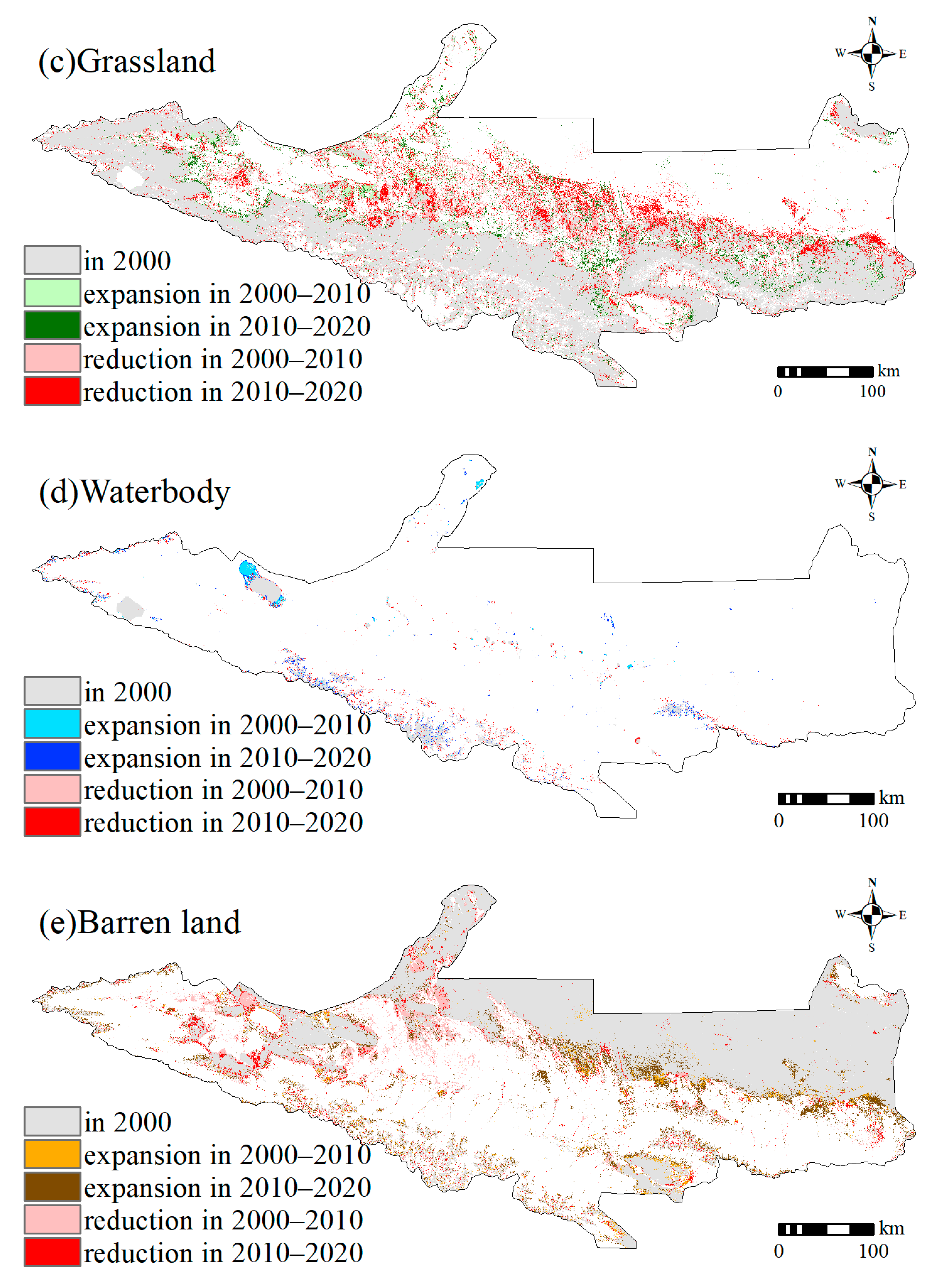
3.1. Land Use Change during 2000–2020

Figure 2 shows the area and dynamic degree of different land use types from 2000 to 2020. Grassland and barren land are the major land use types on the NSTM, with an area of 6.13 × 10⁶ ha and 5.99 × 10⁶ ha, respectively, accounting for 40.8% and 39.9% of the total area, followed by cropland, with an area of 1.99 × 10⁶ ha, accounting for 13.2%. Waterbody, forest, and construction land is smaller, with an area of 4.47 × 10⁵ ha, 3.66 × 10⁵ ha and 1.07 × 10⁵ ha, respectively, accounting for about 3.0%, 2.4%, and 0.7% (Figure 2a). In terms of land use dynamics, all land use types on the NSTM underwent transformations from 2000 to 2020. Noteworthy is the considerable reduction in grassland, registering a dynamic decrease of −10.4%, predominantly reallocated to cropland and barren land. Conversely, construction land witnessed the most substantial growth, surging by 1.88 times, primarily sourced from grassland, barren land, and cropland. Moreover, cropland and forest also showed an increasing trend, escalating by 42.6% and 21.3% correspondingly, mainly transferred from grassland and barren land. The areas of water and barren land remained relatively stable.
Divided into two stages with 2010 as the boundary, the land use changes on the NSTM showed significant differences in different stages (Figure 3). Remarkably, the surge in cropland predominantly unfolded in the first stage, notably propelled by a remarkable increment in the Tacheng region, registering a dynamic shift of 35.56%. The dynamics of the forest preserved a semblance of constancy throughout the two phases, maintaining a dynamic equilibrium of approximately 10.58%. Grassland witnessed a consistent decline in both phases, with a faster decrease in the first phase, especially in Changji Prefecture. The waterbody exhibited an augmentation during the primary phase followed by a subsequent downturn in the succeeding phase, albeit with a growth momentum surpassing the rate of decline. Noteworthy is the expansion of construction land in both segments, with the growth pace in the initial phase exceeding that of the latter phase by a factor of 2.03. In terms of area change, the most pronounced expansion materialized in cropland between the years 2000 and 2020, boasting a surge of 6.70 × 10⁵ ha, whereby the increment in the initial phase outpaced that of the latter phase by a factor of 5.08. Meanwhile, construction land and forest witnessed increments of 1.04 × 10⁵ ha and 7.03 × 10⁴ ha, respectively, sustaining relatively consistent growth trajectories in both periods. Conversely, the augmentation in waterbodies was the most modest, escalating merely by 3.88 × 10⁴ ha. Subsequently, both grassland and barren land incurred reductions of 6.66 × 10⁵ ha and 2.17 × 10⁵ ha, respectively, with grassland displaying a prolonged decline and experiencing a reduction approximately 2.85 times more in the latter phase than in the initial. Notably, barren land underwent a decline in the preliminary phase followed by a resurgence in the subsequent phase, albeit with the increment being only half the magnitude of the initial decrease (Figure 4).

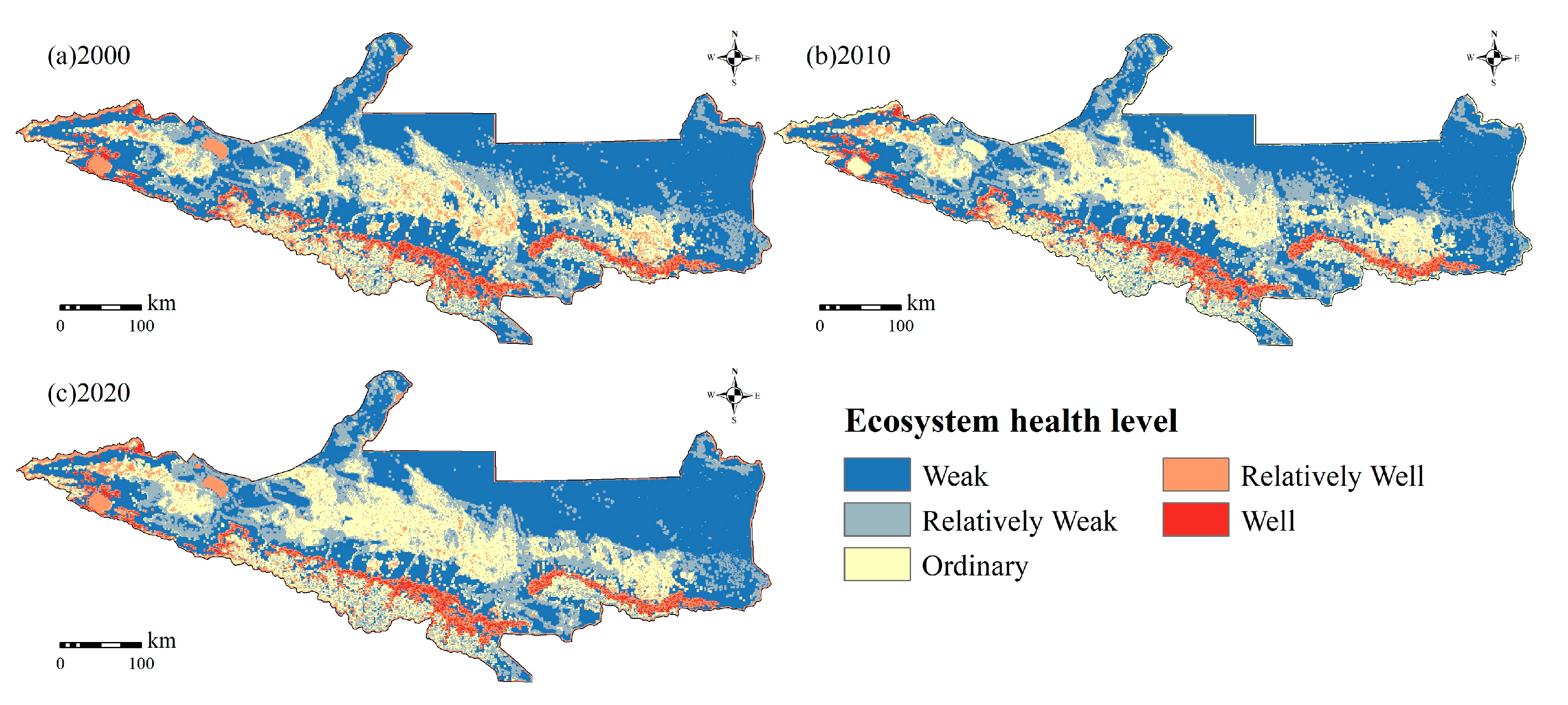
3.2. Analysis of Spatiotemporal Variations in Ecosystem Health

The average EH level rose from 0.1317 in 2000 to 0.1414 in 2020, indicating a gradual improvement in the overall health of the NSTM ecosystem despite its initial low state. In terms of spatial distribution (Figure 5), the zone with a weak level was the most extensive, with an area of about 6.63 × 10⁶ ha and a proportion of 44.1%. This concentration was predominantly observed in the northeast, characterized by barren land and grassland. Areas classified as ordinary and relatively weak encompassed 3.70 × 10⁶ ha and 2.86 × 10⁶ ha, accounting for 24.6% and 19.0%, respectively. These areas are predominantly situated in the central and western regions, characterized by a mix of cropland and grassland. The distribution of relatively well and well areas covered smaller extents, with only 1.44 × 10⁶ ha and 4.03 × 10⁵ ha, representing 9.6% and 2.7%, respectively, mainly concentrated in the south and characterized by forest. In terms of a temporal perspective (Figure 6), from 2000 to 2020, the extent of deteriorating EH areas was 2.49 times greater than that of areas showing improvement. Deterioration primarily occurred in Changji Autonomous Prefecture, characterized by barren land dominance, while improvements were concentrated in the central and southern regions, aligning closely with the spatial prevalence of grassland and forest. While the area of zones categorized as weak and relatively well has declined, those classified as relatively weak, ordinary, and well have expanded, indicating an overall improving yet somewhat unstable trend in NSTM’s EH. Based on the average value of the EH (Figure 7), the ranking of various land categories from highest to lowest health levels is as follows: forest > waterbody > cropland > construction land > grassland > barren land, with corresponding values of 0.3903, 0.2520, 0.2512, 0.1711, 0.1530, and 0.0588. From 2000 to 2020, the EH of all land categories declined except for grassland and waterbody. Cropland, forest, construction land, and barren land witnessed decreases of 4.3%, 1.7%, 3.3%, and 0.4%, highlighting the pressing need for enhanced protection of the overall ecological environment in the NSTM.

3.3. Formatting of Mathematical Components

Figure 8 illustrates the anticipated land use changes in 2030 within the NSTM across various scenario simulations. Compared with 2020, the area of grassland and waterbody under the four scenarios show a decreasing trend, with an average amount of 4.42 × 10⁵ ha and 7.50 × 10³ ha. The areas of cropland, forest, barren land, and construction land show an increasing trend. The barren land is mostly increasing, with an average increase of 2.32 × 10⁵ ha. Except for the FP scenario, the area of cropland under the other three scenarios shows a weak increasing trend, with an average increase of only 5.64 × 10⁴ ha. This phenomenon is related to China’s prevailing cropland protection policy. Under the FP Scenario, cropland is projected to surge by 3.15 × 10⁵ ha. The growth pattern of forest coverage remains relatively consistent across all scenarios, with an average increase of 3.43 × 10⁴ ha, peaking notably under the EP scenario. The increase in barren land under the four scenarios surpasses that of any other land category, averaging a noteworthy increase of 2.32 × 10⁵ ha, which is intimately tied to the degradation of grassland.
Grassland serves as the main source for the expansion of cropland and barren land. The transfer of grassland to cropland varies across scenarios, with figures of 8.16 × 10⁴ ha, 3038 km2, 1418 km2, and 6.65 × 10⁴ ha for ND, FP, EP, and UD, respectively, while the transition to barren land amounts to 2.56 × 10⁵ ha, 5.65 × 10⁵ ha, 2.03 × 10⁵ ha, and 2.53 × 10⁵ ha. Construction land exhibits a consistent growth pattern in all four scenarios, ranking in ascending order: UD (8.63 × 10⁴ ha) > ND (6.29 × 10⁴ ha) > FP (5.13 × 10⁴ ha) > EP (4.60 × 10⁴ ha). Among the various land categories (Figure 9), construction land demonstrates the highest expansion rate, averaging 38.8%, notably surpassing the rates of other categories, particularly under the UD and ND scenarios. Cropland, forest, and barren land expand at rates of 5.4%, 8.6%, and 3.9%, respectively, while grassland undergoes a comparable reduction at 7.7%. The substantial decrease in grassland area, attributed to its vast expanse, is the most significant among all land categories. Geospatially, the diminishing grassland is predominantly concentrated in the southern region of the NSTM (Urumqi City and Changji Prefecture), coinciding with the expanding barren land zone. Cropland expansion areas are concentrated in the central NSTM, whereas forest land expansion is prominent in the mid to high-altitude regions of the NSTM, and construction land expansion is concentrated in the southern part (Urumqi City) and the central part of the NSTM (Kelamayi City and Shihezi City).

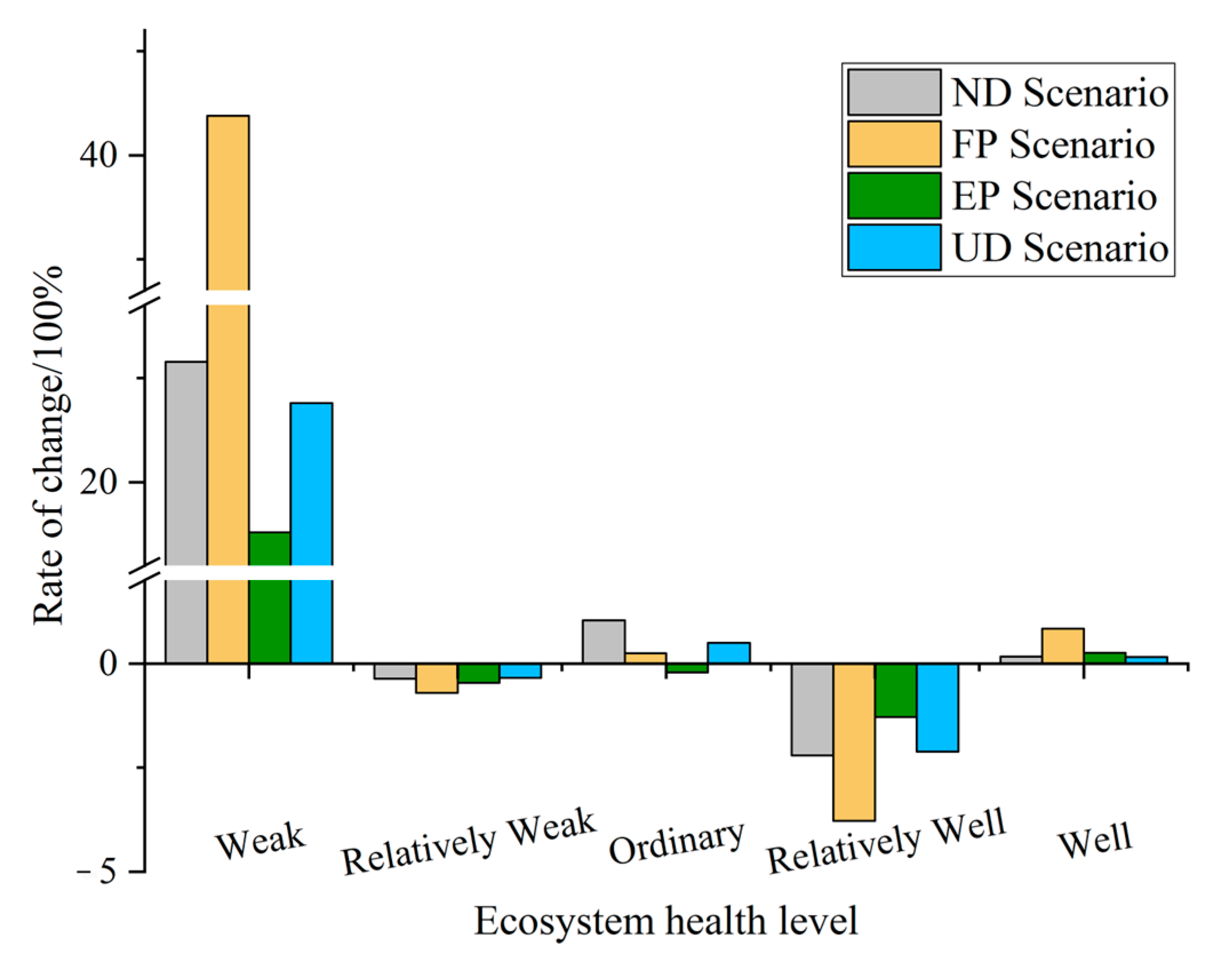
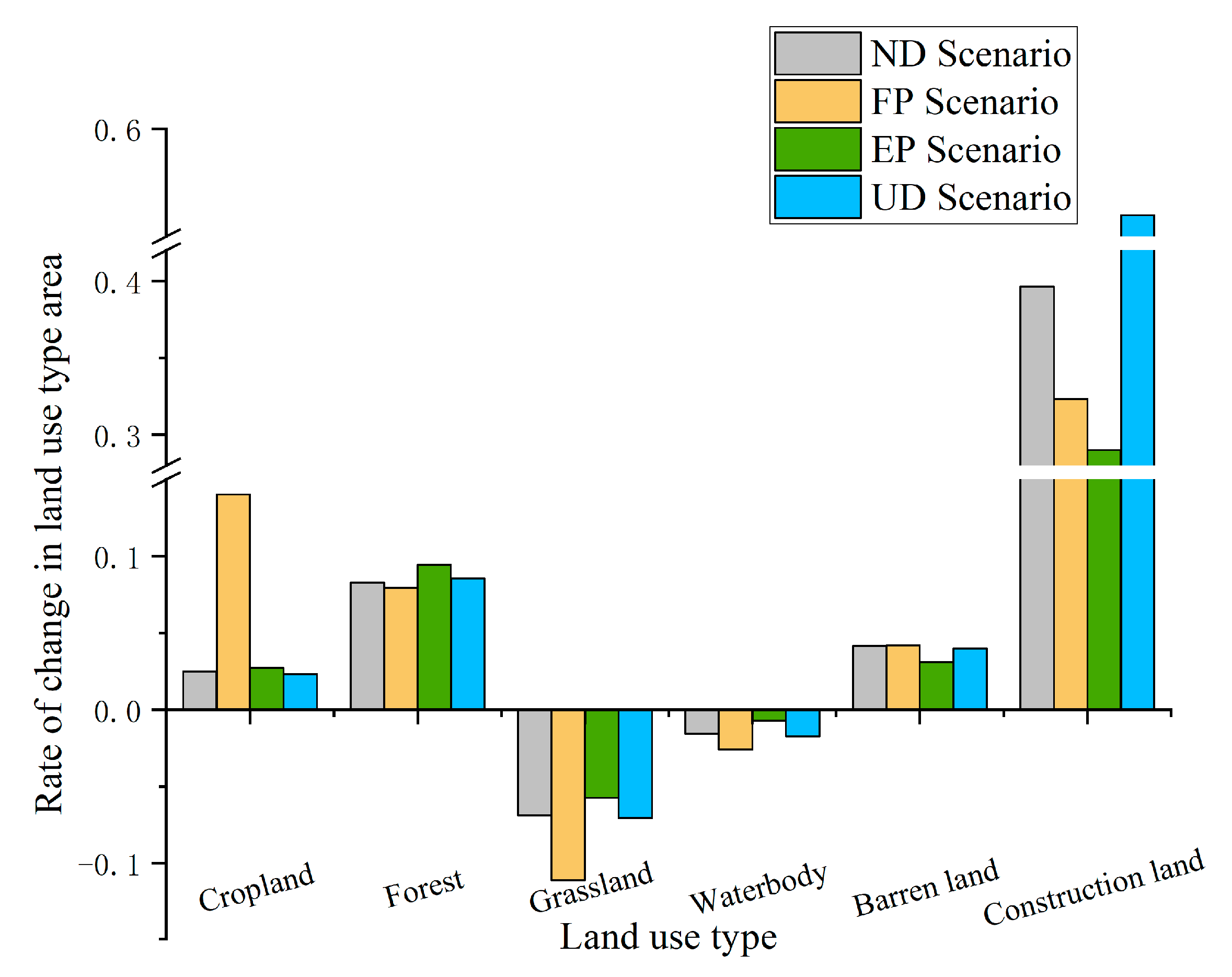
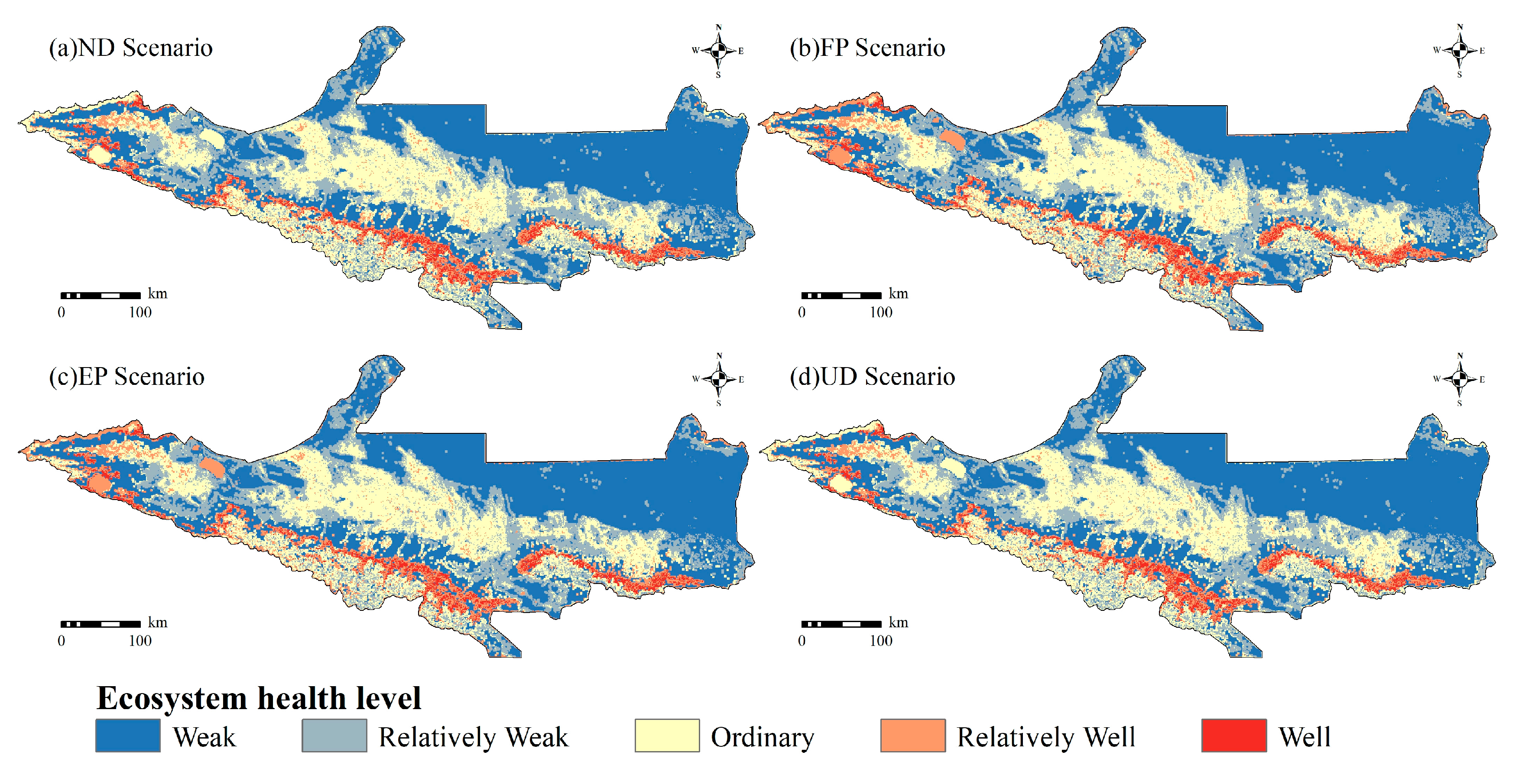
3.4. Prediction of Changes in Ecosystem Health

Figure 10 presents the spatial distribution of EH levels under different scenarios in the NSTM in 2030. The mean values of the EH indices under four scenarios are 0.1386, 0.1455, 0.1402, and 0.1382, respectively (Figure 11). In comparison to 2020, a significant enhancement in EH levels is evident in the FP scenario, while more subtly so in the EP scenario. This is mainly due to the ecological protection priority aiming to minimize the deterioration of the weak level zone. Conversely, a notable decline in EH is observed in both the ND and UD scenarios. The spatial distribution of EH levels remain consistent across scenarios. Well and relatively well level areas are concentrated in the south and west of the NSTM, characterized by forest and grassland. Ordinary level areas are concentrated in the center and south, marked by cropland and grassland. Relatively weak level areas are identified in the barren land of the south and grassland of the southeast, while the weak level area is mainly concentrated in barren land of the north. Significant differences exist in the EH indices among different land use types: forest (0.3845) > waterbody (0.2588) > cropland (0.2418) > grassland (0.1651) > construction land (0.1614) > barren land (0.0572) (Table 2).

3.5. Response of Ecosystem Health to Land Use Change

The elasticity analysis method in economics was introduced in this study to quantify the impact of land use changes on EH. The method measures the sensitivity of EH to land use changes, with higher absolute values indicating greater sensitivity. This means that even small changes in land use can trigger significant changes in EH. In 2020–2030, the ecological elasticity values for the ND, FP, EP, and UD scenarios were −0.3806, −0.0884, −0.3378, and −0.4130, respectively, indicating that the ecological environment of the NSTM is highly fragile. A mere 1% change in land use corresponds to a deterioration in EH of 0.3806%, 0.0884%, 0.3378%, and 0.4130% (Table 3). Under the UD scenario, the absolute value of ecological elasticity of cropland reaches the peak, indicating that urban development has the greatest impact on the EH of cropland. The ecological elasticity of forest was negative in all four scenarios, with the largest absolute values (0.2014; 0.1969) in the ND and UD scenarios, contrasting with the lesser absolutes under the FP and EP scenarios (0.0019 and 0.0356, respectively). This suggests that implementing cropland protection or ecological protection policies can preserve and enhance the EH of forest. Furthermore, the ecological elasticity of grassland has an absolute value greater than 0.3000 in all four scenarios, indicating its vulnerability to land use variations. Although barren land experiences significant negative impacts from land use changes, the cropland protection policy can positively change the trend. Moreover, the ecological elasticity value of construction land is negative under the four scenarios, but the absolute value is relatively low. This suggests that land use changes have a minor impact on the EH in cities and towns.

3.6. Correlation of Ecosystem Indicators

Over recent years, there has been a notable expansion in both the assessment methodologies and conceptual understanding of EH. Nevertheless, despite this evolution, the VOR model introduced by Costanza and Robert [12] remains firmly entrenched and widely embraced within academic circles. Thus, there arises a critical need to assess the relevance of novel indicators when integrating them into the established framework of EHA. The Pearson correlation coefficient serves to quantify both the strength and direction of the linear correlation between two continuous variables, X and Y. To examine the linear correlation between these indicators and EH, we conducted a Pearson correlation analysis utilizing ArcGIS 10.7 Band Collection Statistics Tool within the framework of the VORS model.
Through an evaluation of the Pearson correlation coefficients, we elucidated the extent of contribution that each indicator makes to the outcomes of EH, as depicted in Table 4. EV, EO, ER, and ES exhibited moderately positive correlations with EH (R > 0.4). Notably, EV and ES emerged as the primary contributors to the EH outcomes, aligning with the conclusions drawn by Yan et al. [54] and Ran et al. [55]. In all three years, the correlation coefficients between ES and EH exceeded 0.5, i.e., 0.5793, 0.5815, and 0.5887, respectively. These findings indicate the significance of incorporating ES into the EHA framework to enhance the comprehensive explanatory power of ecosystem assessment.

4. Discussion

4.1. Spatiotemporal Analysis of Ecosystem Health under Different Land Use Scenarios

Upon reviewing the shifts in EH from 2020 to 2030 across the four scenarios, the FP scenario showcases a substantial enhancement compared to the EP scenario. This improvement is chiefly attributed to the expansion of cropland and the enhancement of grassland quality, with cropland proving more resilient to challenging climatic conditions than grassland [56]. In contrast, the EP scenario failed to improve EH significantly even with strict control of land use conversion, suggesting that mere quantity or usage regulation cannot counteract the adverse effects of ecosystem deterioration. The significant decline of EH in both the ND and UD scenarios was due to the unbridled expansion of construction land. Declining ecosystem service capacity [26] and increasing landscape fragmentation [22] brought by rapid urban expansion are the main causes of ecosystem degradation. The comparison of the four scenarios indicates that controlling usage is merely a fundamental measure for preserving EH in the urban agglomerations on the NSTM. To achieve a substantial enhancement in EH, a more holistic approach encompassing rigorous ecological restoration and soil conservation is imperative. The original EH of the NSTM is poor, characterized by the widespread distribution of the Gobi Desert as well as degradation of oases and grasslands. The sparse vegetation makes the ecosystem more sensitive [56] and susceptible to arid climatic influences [57]. That’s why the weak level areas on the NSTM were generally dominated by barren land.

4.2. Management Recommendations Based on Evaluation Results

The transformation of land use driven by human activities has emerged as a widely acknowledged global environmental concern [21]. Being the core of new urbanization, the population growth and spatial spread of urban agglomeration undeniably exert substantial influence on the ecological landscape [58]. This influence is particularly pronounced in the urban agglomeration situated on the NSTM, nestled within an ecologically delicate region in the inland northwest of China. Thus, a comprehensive examination of the ecological well-being of the arid-zone oasis urban agglomerations becomes imperative. Across the quartet of scenarios, the amelioration of ecological robustness appears universally lackluster, with all elasticity metrics sporting a negative trajectory. This underlines the grim reality that the extreme pursuit of either socioeconomic advancement or ecological safeguarding yields detrimental blows to the ecosystems, far from an ideal panacea for upholding ecological well-being. Unraveling the intricate dance between economic ascension and environmental preservation stands as the linchpin for fostering sustainable development along the NSTM. The integrated scenario model is more effective in navigating the delicate equilibrium between ecological stability and economic progress [59]. Broadly speaking, the ecosystem protection of the urban agglomeration along the NSTM demands a multifaceted approach. Primarily, expediting the refinement of ecological conservation mechanisms and spatial planning for national domains is imperative. Rigorous delineation of national territorial spatial blueprints fortify ecological law enforcement, and steadfast guardianship of ecological sanctuaries, environmental thresholds, and sustainable natural resource utilization constitute quintessential endeavors. Secondly, a concerted effort across all societal strata is warranted. Steering towards the adoption of green and low-carbon paradigms, enforcing stringent environmental entry prerequisites, expediting the phasing out of antiquated production capacities, and fostering a culture of green technological breakthroughs stand as pivotal strategies aimed at stemming environmental degradation at its root. Paramount to this endeavor is the bolstering of meticulous ecological stewardship. Elevating water resources and EH level to non-negotiable benchmarks for industrial expansion, urban sprawl, and ecological preservation assumes paramount importance. For example, within low EH zones, stringent controls must be imposed on land use conversions, while curtailing the encroachment and reclamation of forested expanses and grassy knolls. However, the complete prohibition of logging and grazing is untenable, vital for sustaining vegetative biomass proliferation. Concurrently, a diversified portfolio of ecological restoration ventures ought to be embraced. Within middle EH zones, proactive advocacy for rational land use schema stands as an imperative, enhancing the judicious apportionment of terrestrial assets whilst concurrently safeguarding or augmenting ecological well-being. Meanwhile, within high EH zones, judicious infrastructural undertakings remain permissible, albeit with stringent safeguards to preempt ecological harm. Prioritizing the demarcation of ecological demarcation lines, rigorously vetting incoming enterprises, and fostering the proliferation of clean energy sources emerge as indispensable measures in this regard.
Furthermore, intricate interdependencies and trade-offs exist among diverse ESs. When there are changes in climate, policy, and land use, carbon sequestration exhibits substantial synergies with soil and water conservation, but significant trade-offs with water yield [60]. On the other hand, water yield is the only ES indicator displaying significant synergy with agricultural production [59]. The water security predicament on the NSTM has escalated over the past two decades due to the impacts of climate change and human activities, intensifying competition for water allocation across sectors. Expansion of construction land not only encroaches upon agricultural landscapes, but also causes irreversible structural damage to the soil system, impeding multiple ecological service functions like water production, water interception, and carbon sequestration. To promote sustainable socio-economic development in the NSTM, stringent controls on future population growth, industrial expansion, and construction sprawl are recommended. The urban agglomeration should pivot towards green agriculture and eco-industry as the new developmental trajectory, steering towards green advancements through ecological industrialization and industry ecologization.

4.3. Limitations

Based on the framework of multi-model coupling and scenario simulation available in the literature, this study introduced ecosystem services as a pivotal indicator exhibiting the most robust correlation with EH [61] for complementary evaluation, thereby improving the evaluation validity and credibility of the VOR model. Centered around this premise, we selected the urban agglomeration on the NSTM as the study area, exploring the impact of land use and land cover change (LUCC) on EH in arid and semi-arid areas across extensive temporal horizons. The findings presented in this research bear significant weight in enriching our comprehension of the spatial and temporal dynamics governing EH in delicate and vulnerable ecosystems. Furthermore, we utilized the elasticity theory in economics to quantitatively analyze the precise impact of land use change on EH, furnishing policymakers with a more empirical and theoretical foundation to enhance ecological preservation strategies. However, this study encounters certain limitations. Due to the limited accessibility of specific data [62] and the selection of evaluation perspectives [63], comprehensive consideration of the full spectrum of impact indicators proves challenging. Additionally, the use of multi-model prediction increases the uncertainty of the simulation results to a certain extent [21]. Furthermore, the direct impacts of climate change, population, and urban expansion on EH warrant further exploration. Subsequent research should prioritize expanding the array of evaluation metrics and dimensions, culminating in the development of a comprehensive simulation framework.

5. Conclusions

This study delves into the intricate interplay between land use dynamics and ecosystem vitality within the NSTM from 2000 to 2020, amalgamating the PLUS and VORS models to forecast EH trajectories across diverse land use scenarios. Through the application of elasticity analysis, this study quantifies the potential repercussions of land use alterations on EH. The key findings are summarized as follows:
(1)
Land use on the NSTM from 2000 to 2020 was dominated by barren land and grassland. Due to irrational grazing, cropland protection policies, and other reasons, there was a discernible trend of grassland degradation and conversion to cropland and barren land, resulting in a reduction of approximately 10.4%. Concurrently, there was a substantial expansion of construction land by 188%, signaling a deepening urbanization process within the NSTM. While the overall EH status of the NSTM remains predominantly subpar, there is a gradual trend of improvement observed, in which the EH of forest is relatively well, the EH of cropland is ordinary, and the EH of grassland and barren land is relatively weak.
(2)
Under the four simulation scenarios, there is a notable decline in the area of grassland and water bodies, coupled with an increase in cropland, barren land, and construction land areas. The expansion rate of construction land surpasses all other land categories significantly. Due to its initial extensive coverage, the rate of grassland decline is gradual, but the magnitude remains the most substantial.
(3)
In 2020–2030, the trajectory of EH deterioration exhibits signs of improvement or mitigation under the FD and ED scenarios, yet a pronounced degradation is evident under the ND and UD scenarios. Negative ecosystem elasticity is observed across all scenarios, indicating the fragility of the NSTM’s ecological environment. Urgent measures are imperative to uphold the structural and functional stability of its ecosystem. The values of ecological elasticity varied among different land categories, with cropland, barren land, and grassland bearing a heightened susceptibility to the impacts of land use changes, while construction lands, forests, and water bodies demonstrate a lesser vulnerability to such alterations.
The outcomes of this study hold considerable scientific and practical significance: they enhance the application scenarios and internal methodologies of EHA, further validate the soundness of the VORS model, and deepen comprehension regarding the impacts of human activities on EH across arid and non-arid regions. Furthermore, the analysis of changes in EH under diverse land types and policies offers novel insights and scientific references for governments on the NSTM, aiding in their grasp of economic development and ecological stability while shaping environmental governance policies. Given the diverse service functions encompassed by ES, some of which may intersect with natural EH, thorough consideration will be given in future research to the relationship between each ES sub-service and EH, along with other sub-indicators, to prevent redundant evaluations.

Author Contributions

Conceptualization, F.C.; methodology, Z.H.; software, Z.H.; validation, Z.H., F.C. and Y.S.; formal analysis, Z.H.; investigation, Z.H. and Y.Y.; resources, F.C. and X.Z.; data curation, J.M.; writing—original draft preparation, Z.H.; writing—review and editing, F.C. and Y.Y.; visualization, J.M.; supervision, F.C.; project administration, X.Z.; funding acquisition, F.C. All authors have read and agreed to the published version of the manuscript.

Funding

This research was funded by the Major Special Projects of the Third Comprehensive Scientific Exploration in Xinjiang (2022xjkk1005) and the Open Fund of Observation Research Station of Land Ecology and Land Use in the Yangtze River Delta, MNR (No. 2023YRDLELU01).

Data Availability Statement

The data presented in this study are available on request from the corresponding author. The data are not publicly available to protect the privacy of the study’s participants.

Conflicts of Interest

The authors declare no conflicts of interest.

References

  1. Costanza, R.; d‘Arge, R.; De Groot, R.; Farber, S.; Grasso, M.; Hannon, B.; Limburg, K.; Naeem, S.; O’neill, R.V.; Paruelo, J. The value of the world’s ecosystem services and natural capital. Nature 1997, 387, 253–260. [Google Scholar] [CrossRef]
  2. Peng, J.; Liu, Y.; Wu, J.; Lv, H.; Hu, X. Linking ecosystem services and landscape patterns to assess urban ecosystem health: A case study in Shenzhen City, China. Landsc. Urban Plan. 2015, 143, 56–68. [Google Scholar] [CrossRef]
  3. Comberti, C.; Thornton, T.F.; De Echeverria, V.W.; Patterson, T. Ecosystem services or services to ecosystems? Valuing cultivation and reciprocal relationships between humans and ecosystems. Glob. Environ. Change 2015, 34, 247–262. [Google Scholar] [CrossRef]
  4. Rao, Y.; Zhang, J.; Wang, K.; Jepsen, M.R. Understanding land use volatility and agglomeration in northern Southeast Asia. J. Environ. Manag. 2021, 278, 111536. [Google Scholar] [CrossRef] [PubMed]
  5. Peng, J.; Liu, Y.; Li, T.; Wu, J. Regional ecosystem health response to rural land use change: A case study in Lijiang City, China. Ecol. Indic. 2017, 72, 399–410. [Google Scholar] [CrossRef]
  6. Wang, P.; Yu, P.; Lu, J.; Zhang, Y. The mediation effect of land surface temperature in the relationship between land use-cover change and energy consumption under seasonal variations. J. Clean. Prod. 2022, 340, 130804. [Google Scholar] [CrossRef]
  7. Dong, L.; Xiong, L.; Lall, U.; Wang, J. The effects of land use change and precipitation change on direct runoff in Wei River watershed, China. Water Sci. Technol. 2015, 71, 289–295. [Google Scholar] [CrossRef] [PubMed]
  8. De Chazal, J.; Rounsevell, M.D. Land-use and climate change within assessments of biodiversity change: A review. Glob. Environ. Chang. 2009, 19, 306–315. [Google Scholar] [CrossRef]
  9. Jin, G.; Deng, X.; Chu, X.; Li, Z.; Wang, Y. Optimization of land-use management for ecosystem service improvement: A review. Phys. Chem. Earth Parts A/B/C 2017, 101, 70–77. [Google Scholar] [CrossRef]
  10. Ellis, E.; Pontius, R. Land-use and land-cover change. Encycl. Earth 2007, 1, 4631. [Google Scholar]
  11. Arowolo, A.O.; Deng, X.; Olatunji, O.A.; Obayelu, A.E. Assessing changes in the value of ecosystem services in response to land-use/land-cover dynamics in Nigeria. Sci. Total Environ. 2018, 636, 597–609. [Google Scholar] [CrossRef]
  12. Costanza, R. Ecosystem health and ecological engineering. Ecol. Eng. 2012, 45, 24–29. [Google Scholar] [CrossRef]
  13. van Bruggen, A.H.; Goss, E.M.; Havelaar, A.; van Diepeningen, A.D.; Finckh, M.R.; Morris, J.G., Jr. One Health-Cycling of diverse microbial communities as a connecting force for soil, plant, animal, human and ecosystem health. Sci. Total Environ. 2019, 664, 927–937. [Google Scholar] [CrossRef] [PubMed]
  14. Song, W.; Deng, X. Land-use/land-cover change and ecosystem service provision in China. Sci. Total Environ. 2017, 576, 705–719. [Google Scholar] [CrossRef] [PubMed]
  15. Laliberte, E.; Wells, J.A.; DeClerck, F.; Metcalfe, D.J.; Catterall, C.P.; Queiroz, C.; Aubin, I.; Bonser, S.P.; Ding, Y.; Fraterrigo, J.M. Land-use intensification reduces functional redundancy and response diversity in plant communities. Ecol. Lett. 2010, 13, 76–86. [Google Scholar] [CrossRef] [PubMed]
  16. Change, M.B. Global Biodiversity Scenarios for the Year 2100. Science 2000, 287, 1770–1774. [Google Scholar] [CrossRef]
  17. Torres, R.; Gasparri, N.I.; Blendinger, P.G.; Grau, H.R. Land-use and land-cover effects on regional biodiversity distribution in a subtropical dry forest: A hierarchical integrative multi-taxa study. Reg. Environ. Chang. 2014, 14, 1549–1561. [Google Scholar] [CrossRef]
  18. Ma, K.; Kong, H.; Guan, W.; Fu, B. Ecosystem health assessment: Methods and directions. Acta Ecol. Sin. 2001, 21, 2106–2116. [Google Scholar]
  19. Peng, J.; Wang, Y.; Wu, J.; Zhang, Y. Evaluation for regional ecosystem health: Methodology and research progress. Acta Ecol. Sin. 2007, 27, 4877–4885. [Google Scholar] [CrossRef]
  20. Costanza, R. Toward and operational definition of ecosystem health. In Frontiers in Ecological Economics; Edward Elgar Publishing: Cheltenham, UK, 1997; pp. 75–92. [Google Scholar]
  21. Pan, Z.; He, J.; Liu, D.; Wang, J. Predicting the joint effects of future climate and land use change on ecosystem health in the Middle Reaches of the Yangtze River Economic Belt, China. Appl. Geogr. 2020, 124, 102293. [Google Scholar] [CrossRef]
  22. Xie, X.; Fang, B.; Xu, H.; He, S.; Li, X. Study on the coordinated relationship between Urban Land use efficiency and ecosystem health in China. Land Use Policy 2021, 102, 105235. [Google Scholar] [CrossRef]
  23. Yushanjiang, A.; Zhang, F.; Tan, M.L. Spatial-temporal characteristics of ecosystem health in Central Asia. Int. J. Appl. Earth Obs. Geoinf. 2021, 105, 102635. [Google Scholar] [CrossRef]
  24. Samie, A.; Deng, X.; Jia, S.; Chen, D. Scenario-based simulation on dynamics of land-use-land-cover change in Punjab Province, Pakistan. Sustainability 2017, 9, 1285. [Google Scholar] [CrossRef]
  25. Krause, A.; Haverd, V.; Poulter, B.; Anthoni, P.; Quesada, B.; Rammig, A.; Arneth, A. Multimodel analysis of future land use and climate change impacts on ecosystem functioning. Earth’s Future 2019, 7, 833–851. [Google Scholar] [CrossRef]
  26. Li, W.; Wang, Y.; Xie, S.; Cheng, X. Spatiotemporal evolution scenarios and the coupling analysis of ecosystem health with land use change in Southwest China. Ecol. Eng. 2022, 179, 106607. [Google Scholar] [CrossRef]
  27. Kucsicsa, G.; Popovici, E.-A.; Bălteanu, D.; Grigorescu, I.; Dumitraşcu, M.; Mitrică, B. Future land use/cover changes in Romania: Regional simulations based on CLUE-S model and CORINE land cover database. Landsc. Ecol. Eng. 2019, 15, 75–90. [Google Scholar] [CrossRef]
  28. Jiang, L.; Wang, Z.; Zuo, Q.; Du, H. Simulating the impact of land use change on ecosystem services in agricultural production areas with multiple scenarios considering ecosystem service richness. J. Clean. Prod. 2023, 397, 136485. [Google Scholar] [CrossRef]
  29. Zhao, Y.; He, L.; Bai, W.; He, Z.; Luo, F.; Wang, Z. Prediction of ecological security patterns based on urban expansion: A case study of Chengdu. Ecol. Indic. 2024, 158, 111467. [Google Scholar] [CrossRef]
  30. Liang, X.; Guan, Q.; Clarke, K.C.; Liu, S.; Wang, B.; Yao, Y. Understanding the drivers of sustainable land expansion using a patch-generating land use simulation (PLUS) model: A case study in Wuhan, China. Comput. Environ. Urban Syst. 2021, 85, 101569. [Google Scholar] [CrossRef]
  31. Ariken, M.; Zhang, F.; Liu, K.; Fang, C.; Kung, H.-T. Coupling coordination analysis of urbanization and eco-environment in Yanqi Basin based on multi-source remote sensing data. Ecol. Indic. 2020, 114, 106331. [Google Scholar] [CrossRef]
  32. Yibo, Y.; Ziyuan, C.; Simayi, Z.; Shengtian, Y. The temporal and spatial changes of the ecological environment quality of the urban agglomeration on the northern slope of Tianshan Mountain and the influencing factors. Ecol. Indic. 2021, 133, 108380. [Google Scholar] [CrossRef]
  33. Fang, C.; Gao, Q.; Zhang, X.; Cheng, W. Spatiotemporal characteristics of the expansion of an urban agglomeration and its effect on the eco-environment: Case study on the northern slope of the Tianshan Mountains. Sci. China Earth Sci. 2019, 62, 1461–1472. [Google Scholar] [CrossRef]
  34. Tu, A.; Xie, S.; Li, Y.; Liu, Z.; Shen, F. Effect of fixed time interval of rainfall data on calculation of rainfall erosivity in the humid area of south China. Catena 2023, 220, 106714. [Google Scholar] [CrossRef]
  35. Efthimiou, N. The importance of soil data availability on erosion modeling. Catena 2018, 165, 551–566. [Google Scholar] [CrossRef]
  36. Yan, F.; Shangguan, W.; Zhang, J.; Hu, B. Depth-to-bedrock map of China at a spatial resolution of 100 m. Sci. Data 2020, 7, 2. [Google Scholar] [CrossRef] [PubMed]
  37. Yang, J.; Huang, X. The 30 m annual land cover dataset and its dynamics in China from 1990 to 2019. Earth Syst. Sci. Data 2021, 13, 3907–3925. [Google Scholar] [CrossRef]
  38. Chen, X.; He, L.; Luo, F.; He, Z.; Bai, W.; Xiao, Y.; Wang, Z. Dynamic characteristics and impacts of ecosystem service values under land use change: A case study on the Zoigê plateau, China. Ecol. Inform. 2023, 78, 102350. [Google Scholar] [CrossRef]
  39. Costanza, R.; Norton, B.G.; Haskell, B.D. Ecosystem Health: New Goals for Environmental Management; Island Press: Washington, DC, USA, 1992. [Google Scholar]
  40. Li, W.; Wang, Y.; Xie, S.; Cheng, X. Coupling coordination analysis and spatiotemporal heterogeneity between urbanization and ecosystem health in Chongqing municipality, China. Sci. Total Environ. 2021, 791, 148311. [Google Scholar] [CrossRef] [PubMed]
  41. Hernández-Blanco, M.; Costanza, R.; Chen, H.; DeGroot, D.; Jarvis, D.; Kubiszewski, I.; Montoya, J.; Sangha, K.; Stoeckl, N.; Turner, K. Ecosystem health, ecosystem services, and the well-being of humans and the rest of nature. Glob. Chang. Biol. 2022, 28, 5027–5040. [Google Scholar] [CrossRef] [PubMed]
  42. Phillips, L.B.; Hansen, A.J.; Flather, C.H. Evaluating the species energy relationship with the newest measures of ecosystem energy: NDVI versus MODIS primary production. Remote Sens. Environ. 2008, 112, 4381–4392. [Google Scholar] [CrossRef]
  43. He, J.; Pan, Z.; Liu, D.; Guo, X. Exploring the regional differences of ecosystem health and its driving factors in China. Sci. Total Environ. 2019, 673, 553–564. [Google Scholar] [CrossRef] [PubMed]
  44. Xiao, R.; Liu, Y.; Fei, X.; Yu, W.; Zhang, Z.; Meng, Q. Ecosystem health assessment: A comprehensive and detailed analysis of the case study in coastal metropolitan region, eastern China. Ecol. Indic. 2019, 98, 363–376. [Google Scholar] [CrossRef]
  45. Arowolo, A.O.; Deng, X. Land use/land cover change and statistical modelling of cultivated land change drivers in Nigeria. Reg. Environ. Chang. 2018, 18, 247–259. [Google Scholar] [CrossRef]
  46. Allan, A.; Soltani, A.; Abdi, M.H.; Zarei, M. Driving forces behind land use and land cover change: A systematic and bibliometric review. Land 2022, 11, 1222. [Google Scholar] [CrossRef]
  47. Meyfroidt, P.; Lambin, E.F.; Erb, K.-H.; Hertel, T.W. Globalization of land use: Distant drivers of land change and geographic displacement of land use. Curr. Opin. Environ. Sustain. 2013, 5, 438–444. [Google Scholar] [CrossRef]
  48. Zhou, Y.; Li, X.; Liu, Y. Land use change and driving factors in rural China during the period 1995-2015. Land Use Policy 2020, 99, 105048. [Google Scholar] [CrossRef]
  49. Chang, X.; Zhang, F.; Cong, K.; Liu, X. Scenario simulation of land use and land cover change in mining area. Sci. Rep. 2021, 11, 12910. [Google Scholar] [CrossRef] [PubMed]
  50. Huang, D.; Huang, J.; Liu, T. Delimiting urban growth boundaries using the CLUE-S model with village administrative boundaries. Land Use Policy 2019, 82, 422–435. [Google Scholar] [CrossRef]
  51. Wang, Z.; Guo, M.; Zhang, D.; Chen, R.; Xi, C.; Yang, H. Coupling the Calibrated GlobalLand30 Data and Modified PLUS Model for Multi-Scenario Land Use Simulation and Landscape Ecological Risk Assessment. Remote Sens. 2023, 15, 5186. [Google Scholar] [CrossRef]
  52. Wu, J.; Luo, J.; Zhang, H.; Qin, S.; Yu, M. Projections of land use change and habitat quality assessment by coupling climate change and development patterns. Sci. Total Environ. 2022, 847, 157491. [Google Scholar] [CrossRef] [PubMed]
  53. Kennedy, S.; Linnenluecke, M.K. Circular economy and resilience: A research agenda. Bus. Strategy Environ. 2022, 31, 2754–2765. [Google Scholar] [CrossRef]
  54. Yan, Y.; Zhao, C.; Wang, C.; Shan, P.; Zhang, Y.; Wu, G. Ecosystem health assessment of the Liao River Basin upstream region based on ecosystem services. Acta Ecol. Sin. 2016, 36, 294–300. [Google Scholar] [CrossRef]
  55. Ran, C.; Wang, S.; Bai, X.; Tan, Q.; Wu, L.; Luo, X.; Chen, H.; Xi, H.; Lu, Q. Evaluation of temporal and spatial changes of global ecosystem health. Land Degrad. Dev. 2021, 32, 1500–1512. [Google Scholar] [CrossRef]
  56. Tang, L.; Kasimu, A.; Ma, H.; Eziz, M. Monitoring multi-scale ecological change and its potential drivers in the economic zone of the tianshan mountains’ northern slopes, xinjiang, China. Int. J. Environ. Res. Public Health 2023, 20, 2844. [Google Scholar] [CrossRef] [PubMed]
  57. Pei, H.; Fang, S.; Lin, L.; Qin, Z.; Wang, X. Methods and applications for ecological vulnerability evaluation in a hyper-arid oasis: A case study of the Turpan Oasis, China. Environ. Earth Sci. 2015, 74, 1449–1461. [Google Scholar] [CrossRef]
  58. Chen, W.; Chi, G.; Li, J. The spatial association of ecosystem services with land use and land cover change at the county level in China, 1995–2015. Sci. Total Environ. 2019, 669, 459–470. [Google Scholar] [CrossRef] [PubMed]
  59. Qin, K.; Li, J.; Yang, X. Trade-off and synergy among ecosystem services in the Guanzhong-Tianshui Economic Region of China. Int. J. Environ. Res. Public Health 2015, 12, 14094–14113. [Google Scholar] [CrossRef] [PubMed]
  60. Liu, J.; Li, J.; Qin, K.; Zhou, Z.; Yang, X.; Li, T. Changes in land-uses and ecosystem services under multi-scenarios simulation. Sci. Total Environ. 2017, 586, 522–526. [Google Scholar] [CrossRef] [PubMed]
  61. Ma, J.; Ding, X.; Shu, Y.; Abbas, Z. Spatio-temporal variations of ecosystem health in the Liuxi River Basin, Guangzhou, China. Ecol. Inform. 2022, 72, 101842. [Google Scholar] [CrossRef]
  62. Mo, W.; Wang, Y.; Zhang, Y.; Zhuang, D. Impacts of road network expansion on landscape ecological risk in a megacity, China: A case study of Beijing. Sci. Total Environ. 2017, 574, 1000–1011. [Google Scholar] [CrossRef] [PubMed]
  63. Yang, Y.; Song, G.; Lu, S. Assessment of land ecosystem health with Monte Carlo simulation: A case study in Qiqihaer, China. J. Clean. Prod. 2020, 250, 119522. [Google Scholar] [CrossRef]
Figure 1. General situation of the northern slope of Tianshan mountain (NSTM).
Land 13 00571 g001
Figure 2. Changes in land use area and single land use dynamics on the NSTM from 2000 to 2020. (a) Area of each land use type; (b) dynamic degree of single land use type.
Land 13 00571 g002
Figure 3. Land use map on the NSTM from 2000 to 2020.
Land 13 00571 g003
Figure 4. Land use net changes on the NSTM from 2000 to 2020.
Land 13 00571 g004aLand 13 00571 g004bLand 13 00571 g004c
Figure 5. Level of ecosystem health on the NSTM from 2000 to 2020.
Land 13 00571 g005
Figure 6. Changes in ecosystem health level on the NSTM from 2000 to 2020.
Land 13 00571 g006
Figure 7. Dynamic analysis of the impact of land use change on ecosystem health on the NSTM from 2000 to 2020.
Land 13 00571 g007
Figure 8. Spatial distribution of land use types under four scenarios on the Northern Slope of Tianshan Mountain in 2030.
Land 13 00571 g008
Figure 9. Rates of land use change under four scenarios from 2020 to 2030 on the NSTM in 2030.
Land 13 00571 g009
Figure 10. Level of ecosystem health under four scenarios on the Northern Slope of Tianshan Mountain in 2030.
Land 13 00571 g010
Figure 11. The mean level of ecosystem health under four scenarios from 2020 to 2030.
Land 13 00571 g011
Table 1. Scenarios and descriptions of land use change on the NSTM.
ScenarioScenario Description
Natural Development
(ND)
The ND scenario will exclude policy factors such as urban planning and protection, and only consider the land development status under original natural conditions. Based on the expansion rate of land use types from 2010 to 2020, this study set scales for each category in 2030 by Markov chains method [30].
Farmland Protection
(FP)
Cropland protection is of great significance for ensuring the sustainable development of agriculture. Under the FP scenario, the conversion of cropland to other land types is strictly restricted [49], thereby controlling the loss of cropland.
Ecological Protection
(EP)
EP scenario means strictly controlling the conversion of land types in ecological protection areas [50]. Based on the Markov transfer matrix [51], the probability of transferring cropland to construction land is reduced by 30%, with the portion not converted to construction land being converted to forest; the probability of transferring forest and grassland to construction land is reduced by 50%; the probability of transferring forest to cropland is reduced by 50%; and the probability of transferring barren land to grassland is increased by 30%.
Urban Development
(UD)
As an important link on the Silk Road, the NSTM is experiencing rapid economic development and accelerated urbanization. In this scenario, the probability of the transfer of forest and grassland to construction land increases by 50%.
Table 2. Average ecosystem health index values of land use types on the NSTM in 2030.
Land Use TypesNDFPEPUD
MeanVarMeanVarMeanVarMeanVar
Cropland0.24030.04590.24620.04350.24150.04640.23940.0459
Forest0.38170.12310.38810.12040.38680.12200.38160.1229
Grassland0.16360.14250.17100.14320.16250.14430.16340.1425
Waterbody0.22660.08340.24200.09400.25240.10460.22350.0804
Barren land0.05620.08650.05950.09070.05710.09150.05580.0858
Construction land0.16330.05910.15860.06030.16100.06030.16280.0598
Table 3. Eco-elastic coefficient of different land use types on the NSTM in 2030.
Land Use TypesNDFPEPUD
Cropland−0.79270.0304−0.5409−1.0010
Forest−0.2014−0.0019−0.0356−0.1969
Grassland−0.3649−0.6409−0.3175−0.3402
Waterbody0.30410.04860.06930.5043
Barren land−1.15520.2083−1.0567−1.3854
Construction land−0.0734−0.1751−0.1456−0.0589
Mean−0.3806−0.0884−0.3378−0.4130
Table 4. Pearson correlation of EV, EO, ER, and ES with EH in 2000, 2010, and 2020.
REVEOERES
20000.6080 *0.5135 *0.4076 *0.5793 *
20100.6129 *0.5095 *0.4213 *0.5815 *
20200.6184 *0.5104 *0.4301 *0.5887 *
Note: Two-tailed significance test was used; * significant correlation at the 0.05 level.
Disclaimer/Publisher’s Note: The statements, opinions and data contained in all publications are solely those of the individual author(s) and contributor(s) and not of MDPI and/or the editor(s). MDPI and/or the editor(s) disclaim responsibility for any injury to people or property resulting from any ideas, methods, instructions or products referred to in the content.

