Abstract
Shrinking cities suffer from a decreased level of resident activities. As a result, areas with low levels of resident activities may become breeding grounds for social issues. To ease and prevent social issues, it is important to deploy physical space optimisation strategies to effectively guide the distribution of resident activities in shrinking cities. To support the development of such spatial strategies, this paper introduces machine learning-based methods for analysing the nuanced non-linear relationship between resident activities and physical space in shrinking cities. Utilising dual-scale grids, this study calculates multi-source spatial elements, which are subsequently integrated with resident activity data to construct a gradient boosting decision tree model. It then analyses the weight of different spatial elements’ impacts on resident activities and their nonlinear relationships. The model proposed in this study demonstrates good precision in construing the relationship between resident activities and physical space. Based on the research findings, strategies for different types of spatial development in shrinking cities are drawn out. This paper advocates for the application of this analytical approach before conducting spatial planning in shrinking cities to maximise the effectiveness of spatial development in guiding resident activities.
1. Introduction
Shrinking cities, characterised by decreases in their population [1,2], often experience a decrease in resident activities in urban areas. Such diluted resident activity has led to the emergence of areas marked by scant resident engagement, which often evolve into hotbeds of social problems. These areas disrupt the formerly tightly knitted urban fabric [3], leading to the spatial concentration of certain social groups. This development pattern may further result in social isolation [4] and contributes to an increase in crime rates [2]. In response, a series of spatial development strategies, including demolition, large-scale regeneration, and small-scale design-led intervention, have been implemented to steer resident activities and revitalise these areas. However, only limited numbers of such spatial interventions have effectively achieved this goal [5,6,7]. Therefore, there is an urgent need to understand the relationship between physical space and resident activities in shrinking cities. By gaining a more nuanced understanding of these dynamics, it becomes possible to more effectively steer resident activities through conducting strategic spatial development.
China’s urbanisation process faces severe challenges from urban shrinkage [8,9,10,11]. According to the seventh national census data, there are 48 shrinking cities nationwide [12]. The number of shrinking cities and the degree of shrinkage are expected to continue to grow. The loss of population in these cities has led to a decline in the level of resident activity, especially in cities still undergoing new district construction [13], where resident activity is further diluted in urban space [14]. While shrinking cities in China do not exhibit widespread social issues, proactive spatial interventions are necessary to guide resident activities in order to pre-empt potential problems.
To serve as a basis for such spatial interventions, there is a need to understand the relationship between resident activities and the physical space therein. By delving into this relationship, three critical questions are answered: (1) How are resident activities distributed in shrinking cities in China? (2) Are there identifiable patterns in how resident activities correlate with the physical space? (3) Can urban spatial development be enhanced based on an in-depth understanding of the relationship between resident activities and urban space in shrinking cities? At the current stage, there is a relatively limited in-depth exploration of the complex nature of the relationships between residents’ daily activities and physical space in shrinking cities, which limits our capacity to understand and effectively respond to issues caused by urban shrinkage.
Based on the preceding rationale, this paper sets out to investigate the relationship between resident activities and physical space in an exemplary shrinking city in China. Following this introduction, a literature review is provided to set the theoretical foundation for this paper in Section 2. Then, Section 3 details the methodology, including research data, data preprocessing, and the building and training of the gradient boosting decision tree (GBDT) model. Section 4 presents the results, demonstrating the resident activity distribution pattern, the influences of different spatial elements, and the non-linear relationship between spatial elements and resident activities. Section 5 integrates the research findings with theoretical underpinnings and discusses implications for shrinking cities’ development. Finally, as a conclusion, Section 6 discusses the research’s limitations and the future development of this topic.
2. Literature Review
2.1. Obstacles in Spatial Development in Shrinking Cities
Various types of interventions have been developed and implemented in shrinking cities in different countries [1,15,16]. Chief among these are direct physical interventions, which are used to have an impact on socioeconomic dynamics [17]. Under the uncertain planning paradigm (shifting from facilitating growth to accepting the status of a shrinking city) [18,19,20], and the lack of a systematic understanding of how physical space affects socio-economic activities, various spatial development strategies have been employed yet have struggled to achieve their expected outcomes.
The demolition of vacant buildings has emerged as a key intervention in shrinking cities. Specifically, in the German context, demolition has been identified as the only feasible option for the significant volume of vacant housing requiring refurbishment [1]. Large areas of demolition are undertaken to stabilise other residential areas [21]. This strategy is employed with the anticipation of fostering new land uses [5] or injecting fresh dynamics through the creation of open spaces [22]. Nonetheless, the demolition of vacant structures often occurs rapidly in the absence of a cohesive strategy. Consequently, when new developments stall, demolition leaves many vacant lots underutilised for years or decades [5], exacerbating the erosion of social cohesion in shrinking cities.
Urban space redevelopment serves as another strategic approach within physical spaces to invigorate shrinking cities. There are two primary redevelopment tactics observed in these urban areas, yet both frequently struggle to effectively concentrate residents’ activities. The first type involves large-scale spatial developments aimed at regenerating degrading areas. Despite these efforts, such developments often fail to reenergise declining urban centres and are critiqued for contributing to social polarisation [6]. The second type is design-led intervention implemented on a smaller scale, targeting problematic residential neighbourhoods in the hope of revitalising them [7]. Nonetheless, the capacity of design alone to draw residents back to these areas remains a matter of debate [7].
Considering that current spatial development strategies often fail to generate the desired socio-economic returns, it is essential to employ a more nuanced and in-depth understanding of the relationship between resident activities and urban space in shrinking cities. Such knowledge is crucial for generating systematic guidance in conducting spatial development in shrinking cities.
2.2. Studying Resident Activities and Their Relationship with Physical Space in Shrinking Cities
Residents’ daily activities are of crucial importance in the quality of the development of shrinking cities. Several researchers have focused on the state of residents’ livelihood in shrinking cities [23]. Yet, there has been limited research effort dedicated to understanding the factors that shape the distribution of residents’ activities, especially in relation to the physical urban environment. Several studies have highlighted the close connection between physical space and resident activities in shrinking cities. For instance, abandoned buildings in urban areas are usually related to various types of criminal activities [24], which in turn affect socio-economic vitality on a broader scale. Additionally, improved transportation access and the proliferation of suburban residential areas tend to disperse populations away from central urban zones [25,26]. Despite these insights, the scale on which different spatial development strategies affect resident activities in urban areas remains less understood under the context of urban shrinkage.
Extensive research has analysed the impact of urban physical space on resident activities in general urban settings [27,28,29]. A series of theoretical frameworks aimed at explaining human activities in urban space has been utilised to inform this analysis [30,31,32]. Capitalising on the big data resources generated in the digital era, existing studies have conducted in-depth analyses of resident activities’ characteristics based on various data sources, including mobile phone signalling data [33,34,35], nighttime light data [36,37], location service data [38], social media check-in data [39,40], and transportation card data [41]. Furthermore, scholars have explored various spatial elements that influence resident activities and their respective weights, including building density, urban spatial function, traffic accessibility, and land use type characteristics [42]. In terms of research methods, linear regression based on the least squares method is commonly used [43,44] alongside geographically weighted regression methods to account for spatial heterogeneity in relationships [42,45,46]. However, these methods predominantly assess the linear relationship between physical space and resident activities, overlooking the complexity of the relationship between resident activities and physical space in real-life urban settings. For example, while increased building intensity might initially attract more resident activities to a certain area, surpassing a specific density threshold could inversely affect activity levels [45]. Therefore, relying solely on linear analytical models may not fully capture the intricate connections between resident activities and the physical space in shrinking cities.
Recent studies have leveraged the capacity of machine learning methods that have demonstrated significant advantages in analysing the complex nonlinear relationships between physical space characteristics and resident activities in urban areas [47,48,49,50]. In particular, several machine learning methods excel in analysing datasets that feature a considerable number of outliers and high collinearity [51]. Among them, the GBDT model stands out for its efficacy in studying the relationship between resident activities and urban space. Additionally, machine learning techniques, coupled with data generated from location-based service platforms, facilitate the analysis of the characteristics of small-scale built environments [52,53]. However, these methods have not been widely applied in studies of resident activities in shrinking cities. Ma et al. used machine learning methods to examine the relationship between nighttime resident activities and spatial elements [54]. However, the impact of small-scale built environments’ characteristics on resident activities has not been investigated. Practically, the smaller sizes and lower levels of resident activities in shrinking cities have caused contingency in resident activities and facilities’ locations. Therefore, utilising machine learning methods at a smaller scale to unveil the relationship between resident activities and physical space proves challenging. A method that overcomes contingency in resident activities and facilities’ locations is crucial in order to gain a comprehensive understanding of the relationship between resident activities and physical space in shrinking cities.
3. Methodology
3.1. Research Design: Exploring Resident Activities in Shrinking Cities
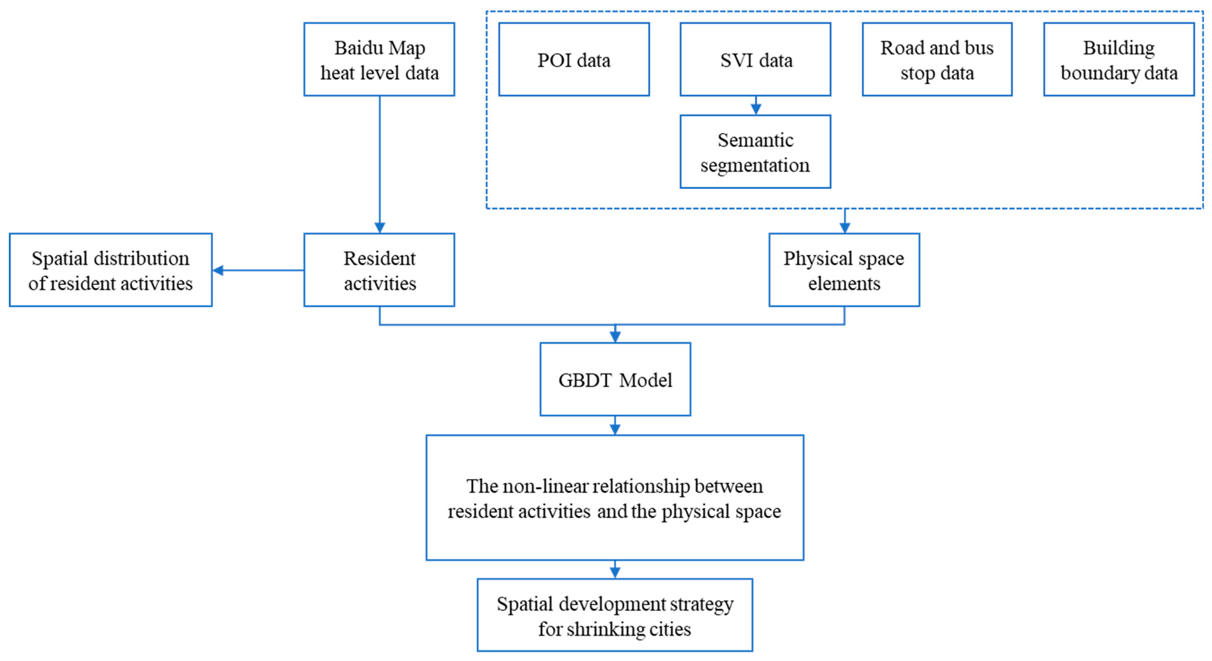
Considering the advantages of machine learning methods and their lack of utilisation in the context of shrinking cities, this study introduces and applies them to the study of resident activities in shrinking cities. The research objective is fulfilled by focusing on the central urban area of Chaoyang City. Firstly, leveraging Baidu heat map data, this paper analyses the spatial distribution of residents’ activities during the day and night on weekdays. Secondly, physical space elements are extracted based on location-based service platforms. The data acquired include street view image (SVI) data, point of interest (POI) data, building boundary data, and road network data, which are used for calculating built environment characteristics, functions and function mix levels, building density, and accessibility. These data are then preprocessed for the building of the GBDT model. Thirdly, based on the physical space and resident activity data, a GBDT model is established to assess the impact weights of different spatial elements on resident activities and the nonlinear relationships among them. Finally, drawing on this analysis, a path is outlined for optimising the physical space of shrinking cities in China and beyond. A flow chart illustrating the research design is shown in Figure 1.
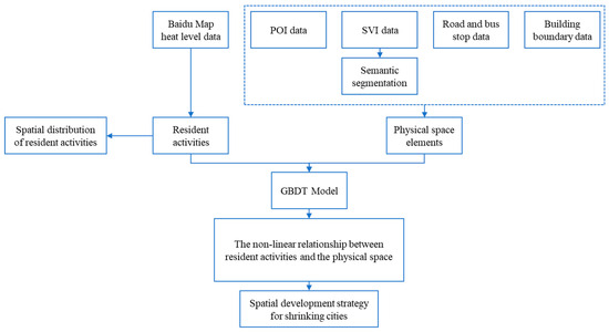
Figure 1.
Flow chart for research design.
3.2. Research Data: Case Selection and Data Acquisition
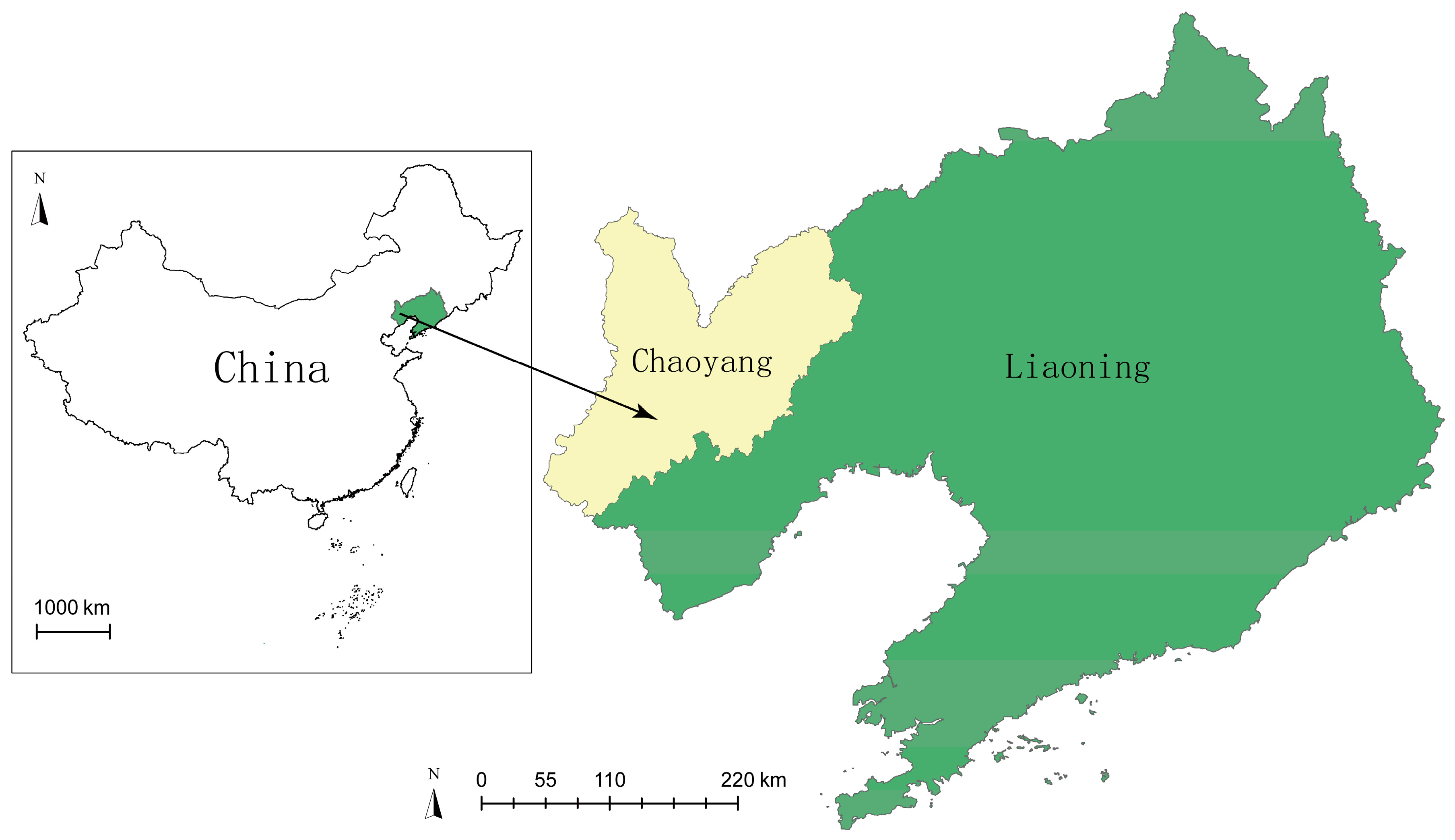
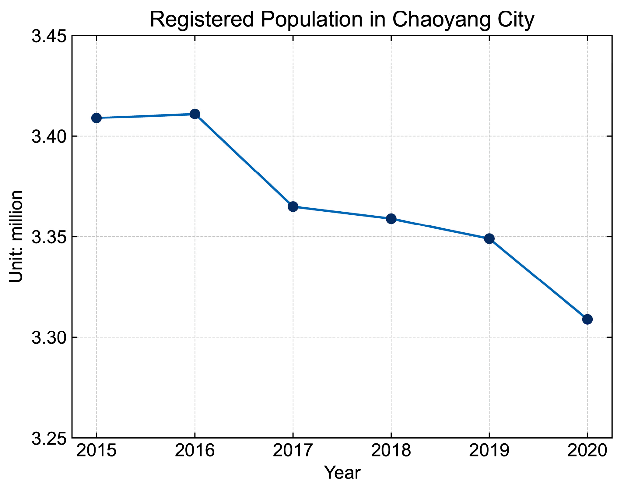
The empirical study presented in this paper focuses on the Chaoyang City, which situates in Liaoning Province of Northeast China (see Figure 2). This city is typical in its development pathway among other shrinking cities in China. Specifically, its historical engagement in heavy industry development has led to challenges in transitioning towards newer economic models. Furthermore, the overall decline of Northeast China sets the broader context for Chaoyang’s development pathway. As a result, the total registered population of the city witnessed a continuous decline, as shown in Figure 3. With a decrease of 10.1% in its permanent population from 2000 to 2020, Chaoyang City can be considered a shrinking city. The central urban area of Chaoyang City with available street view data was selected as the research object. While there is an influx of population into the central urban area, this area exhibits a spatial pattern of being penetrated by a degraded land use status and lower resident activity level under the city’s overall population loss. Furthermore, the built environment in this area is of high construction intensity and has diverse urban spatial functions. Therefore, it is appropriate that we select this case study area for exploring the relationship between resident activities and the physical space in the context of urban shrinkage.
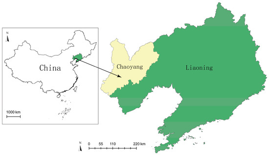
Figure 2.
The location of Chaoyang City.
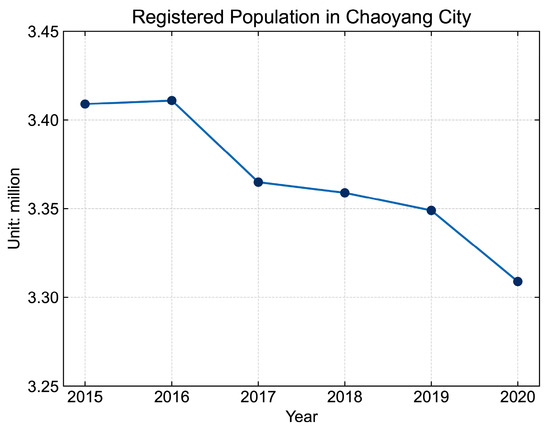
Figure 3.
Registered population in Chaoyang City. Calculated from Liaoning Statistical Yearbook [55].
Regarding the data on resident activities, this study utilised the Baidu Map Open Platform to capture 24 h activity data for each weekday within a week from 16 to 20 October 2023. As for the data on spatial elements, the up-to-date data were acquired in 2023. Based on the Baidu Map platform, the panoramic street view images were captured at 40 m intervals along the roads, providing a foundation for the analysis of small-scale built environment features. Point of interest (POI) data from Chaoyang City were obtained from the Baidu Map Platform, focusing on seven core categories: companies and enterprises, catering services, residences, tourism and sightseeing, shopping, cultural and sports, and scientific research and education. Furthermore, data on urban road networks, bus stop, and building boundaries were obtained from OpenStreetMap to facilitate the analysis of urban spatial accessibility and building density characteristics.
3.3. Data Preprocessing: Overcoming Contingency Caused by Small Sample Sizes
Spatial analysis for data preprocessing was conducted using the ArcGIS 10.8 platform in this study. To develop a model that examines the relationship between resident activities and various elements of the physical space, these elements were processed into standard grids. Two sets of grids were selected: 400 m × 400 m and 200 m × 200 m, with grid counts of 515 and 1297, respectively. Given Chaoyang City is classified as a small-to-medium-sized city with relatively low levels of resident activities and socioeconomic vitality compared to large cities, a set of grids with the resolution of 400 m × 400 m, which is relatively large, were chosen to calculate resident activity levels and POI density. The value of the large grid serves as the feature value for each of its overlapping 200 m × 200 m grids. This approach is utilised to capture the spatial pattern of the distribution of resident activities and POIs, limiting the influences from outliers by diluting their influences to larger areas. When analysing other spatial elements with continuous representation, including the distance to the nearest bus stop, as well as built environment characteristics and road network density, the 200 m × 200 m grid was chosen. This approach allows for a detailed understanding of other spatial elements to be achieved at a finer scale. Thus far, all elements, including resident activity data and various spatial element data, are processed into 200 m × 200 m grids.
Subsequently, data preprocessing was conducted on different spatial elements based on the established grids. Firstly, using the PyCharm integrated development environment, we employed the semantic segmentation algorithm Pyramid Scene Parsing Network (PSPNet) trained with ADE20K dataset to process the SVIs [56,57], focusing on calculating the proportion of different spatial elements in each image. The primary focus was given to analysing the proportions of buildings, sky, trees and grass, earth, motorways, and sidewalks, serving as indicators for building enclosure level, sky openness, green coverage, bare earth proportion, motorway proportion, and sidewalk proportion, respectively. Following this, the average proportion was calculated for each grid, serving as the built environment feature value for the particular grid.
Secondly, road density, the distance from the grid centre to the nearest bus stop, and the proportion of building boundary area were calculated for each grid, serving as the values for different spatial elements. Thirdly, POI densities were calculated for living, working, and leisure space in each grid. Subsequently, the function mix of each grid was calculated based on the number of POIs in the categories of living, working, and leisure. The calculating approach for function mix level, which has been widely used and proven effective in extracting information from urban space [43,46,48], is adopted in this paper. The function mix level is calculated based on the following formula:
wherein represents the proportion of the number of POIs in the ith category and n denotes the number of POI types. Lastly, the overall intensity of resident activities in each grid was calculated, serving as the indicator for resident activities in that grid. For daytime activity levels, the average activity intensity at 10:00, 12:00, 14:00 and 16:00 on weekdays was selected as the representative value. For assessing nighttime activities, the average hourly data from 19:00 to 22:00 on weekdays was selected as the representative value. These time slots were selected with the intention of bringing out a good representation of daytime and nighttime resident activities based on the data we have acquired with limited resources. Descriptions and statistics of resident activities and spatial elements are presented in Table 1.

Table 1.
Descriptions and statistics of resident activities and spatial elements.
3.4. The Construction and Training of the GBDT Model: Unveiling the Non-Linear Relationship
In this study, the GBDT model is selected to analyse the relationship between resident activities and spatial elements. Originally proposed by Friedman [58], the GBDT model consists of multiple decision trees. It continuously fits the negative gradients to improve the accuracy of the results [48] and accumulates the predicted values of the decision trees to achieve model prediction. It is often used in classification and regression models [49].
When constructing the GBDT model, an initial learner is constructed:
where L represents the loss function, denotes the coefficient of the minimum loss function, and N is the total number of samples. Then, the negative gradient value of the loss function of each decision tree is iteratively calculated, serving as its residual estimation [52,59]. The negative gradient is obtained by calculating the negative gradient of the current model at the mth iteration. Based on the negative gradient, a decision tree is fitted, and subsequently, the optimal value resulting in the gradient descent is calculated:
In the model, a learning rate δ (0 < δ ≤ 1) is introduced as a factor of in the step of learner update at the mth iteration to prevent overfitting.
The GBDT model has the advantage of not assuming a linear relationship between the target variable and the explanatory variables, allowing it to determine the weights of different explanatory variables on the target variable based on the fitting results [58,60,61]. At the same time, because it accounts for the relationship between explanatory variables [49], it has a high tolerance for outliers and collinearity. This makes it suitable for analysing the relationship between urban resident activities and spatial elements.
The SHAP (SHapley Addictive exPlanation) model interpreter is used to explain the nonlinear relationship between resident activities and spatial elements in shrinking cities. This concept was introduced in the 1950s based on game theory [62,63]. SHAP has become a commonly used Python package for model interpretation, including in the research fields of urban studies [64,65,66]. It can be used to clarify the positive and negative effects of spatial elements on resident activities at various levels, as well as the nonlinear relationship between physical space elements and resident activities. The impact of feature i on the target variable is represented by the SHAP value of that feature, which is calculated using the following formula:
where N is the set of all features, and S is a subset of N. The term denotes the marginal effect when i is added to S, and M denotes the total number of features.
In this study, the GBDT model was constructed and trained using the Scikit-learn library based on Python. The SHAP interpretation package was employed to analyse the fitting results. The resident activity level serves as the target variable, and the spatial element data serve as the explanatory variable. To prevent overfitting and ensure the model’s generalisation capabilities, a 10-fold cross-validation method was adopted. This involved randomly partitioning the training dataset into 90% for training and 10% for validation to evaluate the model’s fit. A high mean R2 value in a 10-fold cross-validation test indicates a model’s good generalisation capacity, which can be achieved by setting the range of the learning rate [67,68]. The number of trees needs to be adjusted in order to achieve a good prediction result for the model. The grid search approach, which is a commonly applied method to tune parameters [69], was implemented to search through different combinations of parameters for the learning rate and tree counts to find the best combination. The number of decision trees and the learning rate led to high average R2 values in both the 10-fold test and the original data set, which means good capacities were achieved in generalisation and extracting information from the original dataset; these numbers were therefore selected as the optimised model parameters. The optimal number of decision trees was 395, and the learning rate was set to 0.12. The model achieved prediction accuracies of 0.860 and 0.895 for daytime and nighttime resident activity predictions.
4. Results
4.1. Spatial Distribution Patterns of Resident Activities
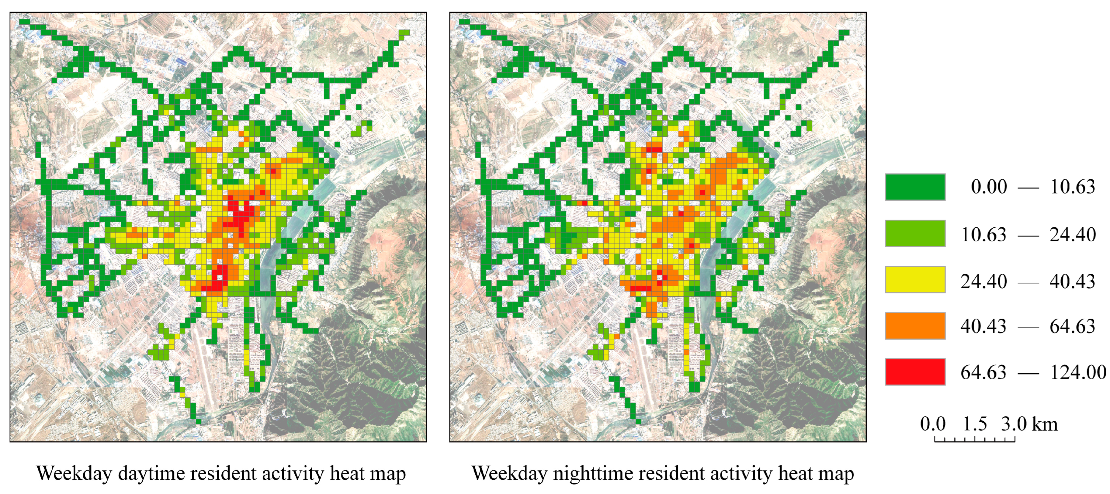
The spatial distribution of resident activities in Chaoyang City is shown in Figure 4. During the daytime, resident activities mainly exhibited a single-centre distribution pattern, characterised by a concentration of high resident activity levels in the central area. As one moves away from this central point, there is a noticeable decline in the level of resident activities. Beyond the central area, there are several scattered areas with higher levels of resident activities. The outer areas present lower levels of resident activities. During the nighttime, the overall level of resident activities is lower than during the day. However, the trend of declining resident activity levels with increased distance from the urban centre persists. Contrary to daytime patterns, hotspots of activity are more scattered throughout the inner city rather than being centrally located, with an augmented count of areas displaying elevated activity levels. The outer area still exhibits lower levels of resident activities.
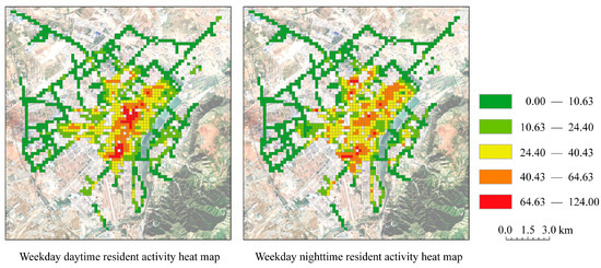
Figure 4.
Spatial distribution of resident activities in Chaoyang City.
4.2. The Weight of Spatial Elements’ Influences on Resident Activities
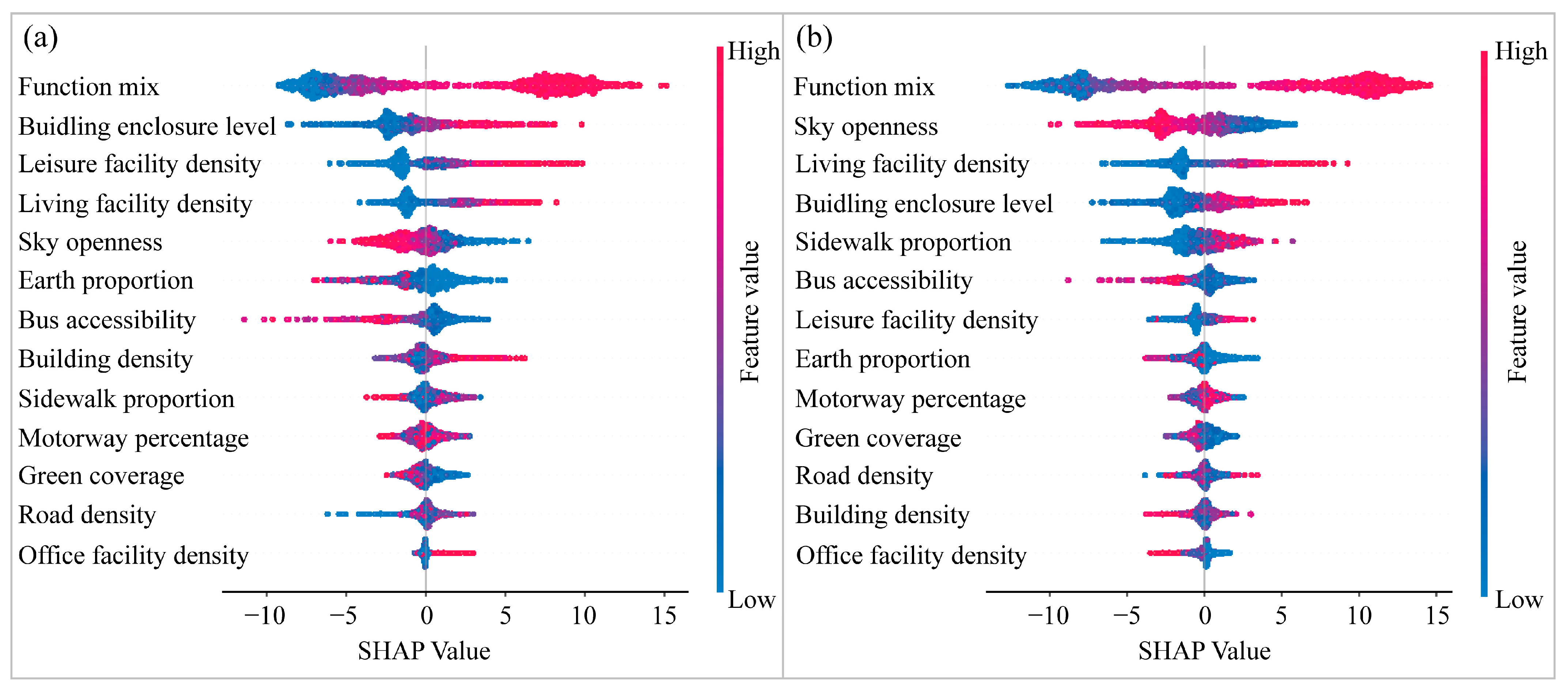
The average SHAP values of different spatial elements that influence resident activities during weekdays (including daytime and nighttime) in Chaoyang City and their rankings can be found in Table 2. Figure 5a illustrates the influences of various spatial elements on resident activities in all the grids discretely during the daytime of weekdays. Among them, the degree of function mix has the most significant impact on resident activities. A higher level of function mix markedly boosts its positive influences on resident activities. In terms of spatial functions, recreational areas and living facilities have a substantial impact on the level of resident activities. Elevated values of these elements correlate with a pronounced positive effect on resident activities, whereas diminished values tend to have a discernible negative impact.
Table 2.
SHAP value and ranking of spatial elements.
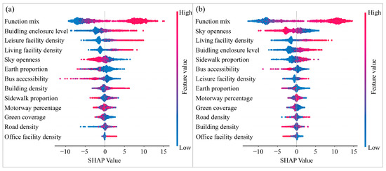
Figure 5.
SHAP value of spatial elements: (a) SHAP value during daytime. (b) SHAP value during nighttime.
Among the built environment characteristics, the building enclosure level stands out as having the greatest influence on resident activities. When the building enclosure level is low, it has a significant negative impact on the concentration of resident activities. Conversely, when building enclosure level is high, the impact turns positive. The sky openness and the bare earth area exhibit a relatively high impact on resident activities. Elevated values for these elements are associated with a negative effect on resident activities. It is particularly noteworthy that, according to the SVIs captured in this study, places with a higher proportion of bare earth are mainly construction sites, dilapidated factories, and large areas of bare land in communities. Typical street view examples with large areas of the three types of bare land are shown in Figure 6. These types of land use are typical brownfield land which has been commonly observed in shrinking cities. Therefore, the observed correlation between bare earth and the negative impact on resident activity concentration highlights the brownfield dilemma in shrinking cities [70], which disrupts the urban social fabric and leads to a decreasing resident activity level. Sidewalks, motorways, and green coverage have relatively low impacts on resident activities.
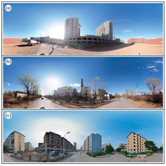
Figure 6.
Examples of SVI with large percentages of exposed earth are (a) construction sites, (b) factory sites, and (c) exposed earth in neighbourhoods.
In terms of accessibility, the distance to the nearest bus stop significantly influences the level of resident activities. As the distance from the bus stop increases, the negative impact on resident activities becomes significantly more potent. Conversely, road density exerts a minimal effect on the intensity of resident activity. Considering the small urban area of Chaoyang City, there is likely a lesser need for extensive road networks, resulting in a minimal association between road density and resident activities. Therefore, emphasising road density might not be crucial in the city’s spatial development initiatives.
The SHAP values of different spatial elements during weekdays at night in Chaoyang City are shown in Figure 5b. Echoing daytime patterns, the degree of spatial function mix stands out as having the greatest influence on resident activities. A high degree of function mix significantly boosts resident activity levels. Regarding spatial functions, living facilities have a significant positive impact on the concentration of resident activities. On the contrary, leisure and office facilities seem to exert minimal influence on the distribution of resident activities.
Among the built environment elements, sky openness, building enclosure level, and the proportion of sidewalks significantly impact nighttime resident activities. A high level of building enclosure markedly enhances resident activities. Conversely, the sky openness tends to detract from resident activities. This correlation is consistent with the commonly observed tendency that residents tend to prefer higher enclosure levels and indoor spaces. Notably, the impact weight of the proportion of sidewalks on resident activities at night is higher compared to the daytime, and there are differences in the impact patterns. At night, a lower proportion of sidewalks has a significant negative impact on the concentration of resident activities, whereas a high proportion leads to a positive impact. This may stem from residents’ tendency to prefer areas with suitable walking spaces at night. Therefore, creating suitable waking spaces can be considered beneficial for attracting resident activities at night and used for preventing potential social issues such as high crime rates in shrinking cities. Although the impact weight of bare earth is not as significant as during daytime, a higher proportion of bare earth still has a significant negative impact on the concentration of resident activities, underscoring the need for addressing land use issues irrespective of the time. In terms of accessibility, both bus stop accessibility and road density play a minor role on residents’ nighttime activities.
4.3. Analysis of Non-Linear Relationships between Physical Spatial Elements and Resident Activities
This section presents the SHAP value patterns for various spatial elements in relative to the spatial elements’ values. In particular, this paper focuses on the spatial elements whose SHAP values potently correlate with the increase of the spatial elements’ values.
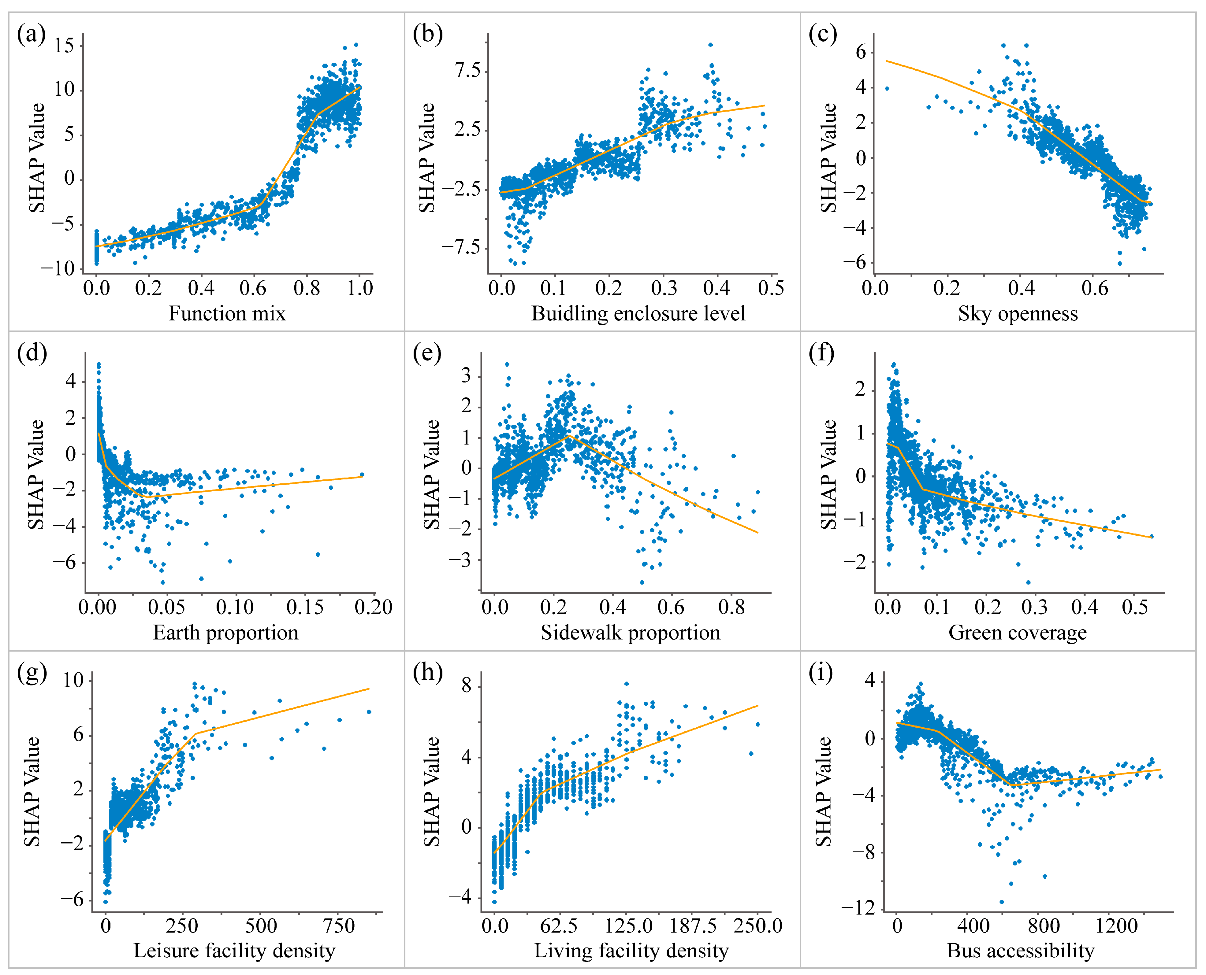
The distribution of SHAP values for various spatial elements during the day on weekdays is shown in Figure 7. The capacity to generate resident activity agglomeration in urban spaces increases with the increase in function mix. When the function mix level reaches 0.84, the growth rate of the agglomeration capacity begins to slow down. This observation suggests that the optimum function mix level is 0.84 during the daytime.
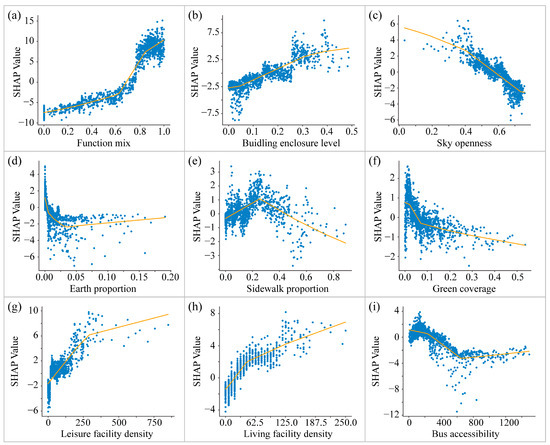
Figure 7.
The SHAP values for different spatial elements in the daytime are shown in (a–i). Only the spatial elements whose SHAP values strongly correlate with the increases of the spatial elements’ values are presented.
Among the various built environment characteristics, the degree of building enclosure signifies a pivotal threshold at 0.39, beyond which the capacity for resident activity agglomeration peaks and then plateaus. For sky openness, a less than 0.57 value enhances the agglomeration of resident activities, but beyond that, such a trend is reversed. This trend highlights the detrimental effect of excessive sky openness on activity concentration. In terms of bare earth, when the proportion is below 0.003, the influence remains ambiguous, but once the proportion reaches 0.003, a negative impact emerges. Such correlation underscores the need for attention to the unused bare land. Sidewalk proportion also exhibits a threshold effect. When the proportion of sidewalks is less than 0.03, the capacity to agglomerate resident activities increases with the increase in the sidewalk proportion. However, after reaching 0.03, the agglomeration capacity begins to decrease gradually. This correlation pattern demonstrates an optimum sidewalk proportion of 0.03 during the day. Lastly, green coverage begins to hinder rather than facilitate concentrating resident activities when exceeding 0.06. It suggests that overly abundant green space may not be conducive to agglomerating resident activities.
In terms of urban spatial functions, leisure functions demonstrate a positive correlation with the intensity of resident activities. However, when the density of leisure facilities reaches 294 per km2, the growth rate of its impact on resident activities begins to decrease, indicating that the optimal capacity for stimulating resident activity agglomeration is achieved at this density in Chaoyang City. Similarly, living facilities positively correlate with resident activities, achieving an effective concentration for resident activities at 43 living facilities per km2. Regarding accessibility characteristics, the negative impact on resident activities is most pronounced at a distance of 655 metres to the bust stop.
The distribution of SHAP values for physical space elements during weekdays at night is shown in Figure 8. The relationship between function mix and residential activities mirrors the daytime one, which is predominantly positive. Notably, when the function mix level reaches 0.80, the growth rate of its impact on the capacity to agglomerate resident activities begins to decline.
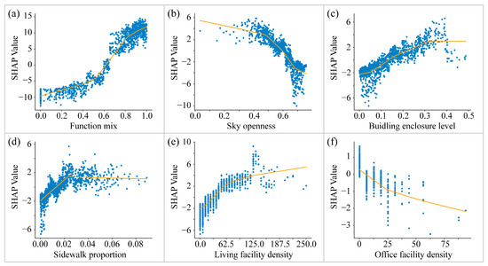
Figure 8.
The SHAP values for different spatial elements in the nighttime are shown in (a–f). Only the spatial elements whose SHAP values strongly correlate with the increases of the spatial elements’ values are presented.
In terms of built environment characteristics, the sky openness continues to have a negative correlation with the agglomeration of resident activities. A specific threshold where sky openness starts to negatively impact resident activity agglomeration is identified at 0.59. Regarding the building enclosure degree, its capacity to agglomerate resident activities increases until its value reaches 0.34. Beyond that, the space’s ability to agglomerate resident activities tends to flatten out. This pattern holds true for both daytime and nighttime, while exhibiting an approximately consistent optimal building enclosure level for maximising resident activity concentration. For sidewalk proportion, when it is less than 0.02, resident activities increase with the increase in the proportion of the sidewalk. After the proportion reaches 0.02, the space maintains a stable agglomeration ability for resident activities. Therefore, when the proportion of the sidewalk is 0.02, it achieves the best effect of concentrating resident activities at night.
In terms of spatial functions, the intensity of residential activities increases with the densification of living facilities, culminating in an optimal density at 69 living facilities per km2. Beyond this point, living facilities’ capacity to concentrate resident activities reaches a plateau. A negative correlation is observed between the concentration of resident activities at night and the density of work facilities. This trend underscores a disconnection between working and residential areas in Chaoyang City, suggesting that too dense a concentration of workspaces may detract from the vibrancy of resident activities during nighttime.
5. Discussion: Towards an Enhanced Spatial Development Strategy
The empirical findings reveal that despite experiencing an overall population decline, the city centre remains attractive for local people to conduct daily activities. The city centre’s capacity to agglomerate resident activities is more evident during the daytime. Outside the city centre, areas with lower- and higher-level resident activities nestle close to one another. Nevertheless, the outer area is relatively less attractive for residents to conduct activities. Overall, resident activities paint a picture of urban patchwork [71], where the city centre remains a relatively heated area; a discrete distribution pattern outside the city centre is observed; and low levels of resident activities are found in the outer urban area. It tangentially adheres to the shrinkage pattern identified by researchers through the layering of punctuation and suburban shrinkage types.
The GBDT model applied in this research illustrates how physical space elements contribute to a distinct urban patchwork of resident activities. Based on the correlation between spatial elements and resident activities, implications for different spatial development strategies in Chaoyang City can be drawn out. The research findings underscore the minimal influence of building density, reflected through the base area of buildings, on resident activities in shrinking cities. Therefore, a pro-growth spatial development strategy that aims to continue increasing building density in the city’s inner and peripheral areas would tend to be ineffective in generating higher levels of resident activities in shrinking cities. This echoes problematic attempts to revitalise cities through deploying pro-growth urban development in shrinking cities in China [13,72] and beyond [73].
Among the built environment’s characteristics, a positive correlation is found between the building enclosure level and resident activities. Meanwhile, sky openness bears a negative correlation with resident activities. Therefore, demolition in shrinking cities that would significantly alter the building enclosure level and sky openness needs to be conducted with much caution, echoing concerns raised by multiple researchers [22]. Irrational demolition risks diminishing building encloser levels and enlarging sky openness, potentially leading to a decrease in population activities in its surrounding area. Furthermore, as resident activities are negatively associated with bare land in shrinking cities, the temporarily unused land resulting from demolition may further dampen the space’s capacity to draw in resident activities. As a result, the primary goal of reducing social issues through large-scale demolition [1] is likely to be undermined if a more deliberate and strategic demolition approach is absent.
Small-scale design-led spatial development can be conducted in shrinking cities based on in-depth explorations of the intricate relationship between physical space and resident activities. For example, potential exists in small-scale spatial interventions that increase building enclosure levels, such as using decorative walls, to attract residents to conduct activities in the surrounding area. Meanwhile, given large areas of bare land lead to significant negative impacts on resident activities in shrinking cities, priority should be given to rectifying brownfield sites, such as unfinished construction sites, dilapidated factories, and unfinished roads in residential areas, to mitigate their divisive impact on socio-economic activities. Moreover, smaller green spaces can be used to increase the space’s capacity in agglomerating resident activities. Finally, acknowledging temporal differences in the correlation between resident activities and spatial elements is important. Despite the fact that the sidewalk does not have strong influence during the daytime, its influence is significant at night. Therefore, creating adequate walking space is beneficial for improving safety levels at night in problematic neighbourhoods through fostering bottom-up street-level monitoring [30].
The regeneration of physical space should also focus on elements apart from the built environment in order to foster vibrant spaces in shrinking cities. The spatial function mix is of the highest importance in generating agglomeration in resident activities during both day and night. This means that a balanced living, leisure, and working space is effective in directing resident engagement. References should be drawn from the city’s optimum function mix level of approximately 0.8 to agglomerate resident activities. Considering the high impact of living space in agglomerating resident activities during both day and night times, guaranteeing land use for living activities can be conducive to creating lively neighbourhoods. The effect of agglomerating resident activities flattens out when living facilities further increase after reaching their optimum value of 43 and 69 during day and night, respectively. These thresholds should be considered when planning to introduce living facilities in different localities of the city with the aim of attracting resident activities. While connectivity tends to drive the outmigration of residents in shrinking cities [25,26], this spatial pattern is not evident regarding resident activities. In this case study, road density is not strongly related to resident activities, while adjacency to bus routes has a greater effect on attracting resident activities. Therefore, increasing road density should not be a high priority in spatial development strategies for shrinking cities. Instead, a meticulously planned distribution of bus routes and stations could better serve as a catalyst for guiding resident activities.
6. Conclusions
To lay the foundation for spatial development in shrinking cities, this paper investigates the relationship between resident activities and physical space in the context of urban shrinkage. Recognising the intricate nonlinear relationship between resident activities and the physical space in shrinking cities, we consider that traditional linear relationship models may fall short in fully capturing their relationships. Furthermore, the use of machine learning methods may be influenced by the contingency in resident activities and facility locations brought by their small sample sizes in shrinking cities. To navigate these complexities, our investigation utilises machine learning methods tailored to the specific nuances of shrinking cities. By using two sets of grids with different sizes to calculate different indicators, our approach effectively addresses the variability in resident activities and the small number of facilities in shrinking cities. The GBDT model constructed in this study demonstrates high precision in analysing the relationship between resident activities and the physical space in the case city, revealing critical insights into how various physical space elements affect resident activities. These findings provide an essential reference for future research and inform urban planning practices related to resident activities in shrinking cities.
The findings generated by this model have the potential to shed light on the development of shrinking cities. It is suggested that an analysis should be conducted to facilitate a systematic understanding of the relationship between resident activities and urban space before initiating spatial development in shrinking cities. By elucidating the effect and identifying the optimal values of various spatial elements in clustering resident activities, a more nuanced approach to spatial development is facilitated. References can be drawn from this knowledge to inform spatial development to enhance its capacity in guiding resident activities. In this sense, employing this informed approach enables a more targeted intervention to achieve goals such as mitigating social issues in shrinking cities.
Finally, there remain limitations to this study that require further research. First, although the model achieves a good level of generalisation in the case study, the relationship between spatial elements and resident activities needs to be further examined across other shrinking cities. Expanding the research scope would foster a more systematic understanding of the interplay between spatial elements and resident activities, thereby enhancing urban development strategies tailored to shrinking cities. Second, the city-level analysis conducted in this study does not reach a nuanced understanding of why certain physical space elements relate to resident activities in a specific manner. For example, why green spaces are negatively correlated with resident activities after reaching a specific value is not fully elucidated and requires further investigation. To address this gap, it is suggested that more granular, small-scale studies be pursued, targeting different individuals’ and social groups’ perceptions of physical space in shrinking cities. By undertaking such detailed investigations, a deeper understanding of residents’ activities and their drives in unique urban contexts can be achieved, offering more contextualised insights so that urban planners and policy makers can guide urban development in shrinking cities.
Author Contributions
Conceptualization, W.Y. and Z.P.; Methodology, F.C.; Software, F.C. and Q.W.; Validation, F.C.; Formal analysis, W.Y. and F.C.; Resources, W.Y.; Data curation, F.C. and Q.W.; Writing—original draft, W.Y.; Writing—review & editing, W.Y., F.C. and Q.W.; Visualization, F.C.; Supervision, Z.P.; Project administration, Z.P.; Funding acquisition, W.Y. All authors have read and agreed to the published version of the manuscript.
Funding
This research was funded by Shanghai Pujiang Program, grant number [21PJC109].
Data Availability Statement
The data presented in this study are available on request.
Conflicts of Interest
The authors declare no conflict of interest.
References
- Schetke, S.; Haase, D. Multi-criteria assessment of socio-environmental aspects in shrinking cities. Experiences from eastern Germany. Environ. Impact Assess. Rev. 2008, 28, 483–503. [Google Scholar] [CrossRef]
- Hollander, J.B.; Pallagst, K.; Schwarz, T.; Popper, F.J. Planning shrinking cities. Prog. Plan. 2009, 72, 223–232. [Google Scholar]
- Ringel, F. Post-industrial times and the unexpected: Endurance and sustainability in Germany’s fastest-shrinking city. J. R. Anthropol. Inst. 2014, 20, 52–70. [Google Scholar] [CrossRef]
- Großmann, K.; Bontje, M.; Haase, A.; Mykhnenko, V. Shrinking cities: Notes for the further research agenda. Cities 2013, 35, 221–225. [Google Scholar] [CrossRef]
- Mallach, A. Demolition and preservation in shrinking US industrial cities. Build. Res. Inf. 2011, 39, 380–394. [Google Scholar] [CrossRef]
- Weaver, R. Palliative planning in an American shrinking city—Some thoughts and preliminary policy analysis. Community Dev. 2017, 48, 436–450. [Google Scholar] [CrossRef]
- Gripaios, P. The failure of regeneration policy in Britain. Reg. Stud. 2002, 36, 568–577. [Google Scholar] [CrossRef]
- Long, Y.; Wu, K.; Wang, J. Shrinking cities in China. Mod. Urban Res. 2015, 9, 14–19. [Google Scholar]
- Li, X.; Wu, K.; Long, Y.; Li, Z.; Luo, X.L.; Zhang, X.L.; Wang, D.; Yang, D.; Gui, Y.; Li, Y. Academic debates upon shrinking cities in China for sustainable development. Geogr. Res. 2017, 36, 1997–2016. [Google Scholar]
- Wu, K.; Long, Y.; Yang, Y. Urban shrinkage in the Beijing-Tianjin-Hebei region and Yangtze River Delta: Pattern, trajectory and factors. Mod. Urban Res. 2015, 9, 26–35. [Google Scholar]
- Yang, W. Pro-growth urban policy implementation vs. urban shrinkage: How do actors shift policy implementation in shrinking cities in China? Cities 2023, 134, 104157. [Google Scholar] [CrossRef]
- Qi, W.; Liu, Z.; Liu, S.; Wu, K.; Wang, X.; Jin, H.; Li, Y.; Wei, H. Identifying shrinking cities in China from 2010 to 2020 based on resident population in physical urban area. Geogr. Res. 2023, 42, 2539–2555. [Google Scholar]
- Yang, D.; Long, Y.; Yang, W.; Sun, H. Losing population with expanding space: Paradox of urban shrinkage in China. Mod. Urban Res. 2015, 9, 20–25. [Google Scholar]
- Long, Y.; Wu, K. Several emerging issues of China’s urbanization: Spatial expansion, population shrinkage, low-density human activities and city boundary delimitation. Urban Plan. Forum 2016, 2, 72–77. [Google Scholar]
- Bernt, M. Partnerships for demolition: The governance of urban renewal in East Germany’s shrinking cities. Int. J. Urban Reg. Res. 2009, 33, 754–769. [Google Scholar] [CrossRef]
- Ortiz-Moya, F. Coping with shrinkage: Rebranding post-industrial Manchester. Sustain. Cities Soc. 2015, 15, 33–41. [Google Scholar] [CrossRef]
- Mallach, A.; Haase, A.; Hattori, K. The shrinking city in comparative perspective: Contrasting dynamics and responses to urban shrinkage. Cities 2017, 69, 102–108. [Google Scholar] [CrossRef]
- Haase, A.; Nelle, A.; Mallach, A. Representing urban shrinkage—The importance of discourse as a frame for understanding conditions and policy. Cities 2017, 69, 95–101. [Google Scholar] [CrossRef]
- Lang, T. Conceptualizing urban shrinkage in East Germany: Understanding regional peripheralization in the light of discursive forms of region building. In Peripheralization: The Making of Spatial Dependencies and Social Justice; Fischer-Tahir, A., Naumann, M., Eds.; Springer: Wiesbaden, Germany, 2013; pp. 224–238. [Google Scholar]
- Popper, D.E.; Popper, F.J. Small can be beautiful: Coming to terms with decline. Planning 2002, 68, 20–23. [Google Scholar]
- Wiechmann, T.; Pallagst, K.M. Urban shrinkage in Germany and the USA: A comparison of transformation patterns and local strategies. Int. J. Urban Reg. Res. 2012, 36, 261–280. [Google Scholar] [CrossRef]
- Frazier, A.E.; Bagchi-Sen, S. Developing open space networks in shrinking cities. Appl. Geogr. 2015, 59, 1–9. [Google Scholar] [CrossRef]
- Hollander, J.B.; Nemeth, J. The bounds of smart decline: A foundational theory for planning shrinking cities. Hous. Policy Debate 2011, 21, 349–367. [Google Scholar] [CrossRef]
- Kraut, D. Hanging out the no vacancy sign: Eliminating the blight of vacant buildings from urban areas. New York Univ. Law Rev. 1999, 74, 1139–1177. [Google Scholar]
- Beauregard, R.A. When America Became Suburban; University of Minnesota Press: Minneapolis, MN, USA, 2006. [Google Scholar]
- Couch, C.; Nuissl, H.; Karecha, J.; Rink, D. Decline and sprawl: An evolving type of urban development. Eur. Plan. Stud. 2005, 13, 117–136. [Google Scholar] [CrossRef]
- Liu, Y.; Zhao, P.; Liang, J. Study on urban vitality based on LBS data: A case of Beijing within 6th Ring road. Areal Res. Dev. 2018, 37, 64—69+87. [Google Scholar]
- Yue, W.; Chen, Y.; Zhang, Q.; Liu, Y. Spatial Explicit Assessment of Urban Vitality Using Multi-Source Data: A Case of Shanghai, China. Sustainability 2019, 11, 638. [Google Scholar] [CrossRef]
- Zhang, A.; Li, W.; Wu, J.; Lin, J.; Chu, J.; Xia, C. How can the urban landscape affect urban vitality at the street block level? A case study of 15 metropolises in China. Environ. Plan. B Urban Anal. City Sci. 2021, 48, 1245–1262. [Google Scholar] [CrossRef]
- Jacobs, J. The Death and Life of Great American Cities; Vintage Books: New York, NY, USA, 1961. [Google Scholar]
- Gehl, J. Life Between Buildings: Using Public Space; Van Nostrand Reinhold: New York, NY, USA, 1987. [Google Scholar]
- Lynch, K. The Image of the City; MIT Press: Cambridge, MA, USA, 1960. [Google Scholar]
- Luo, S.; Zhen, F. How to evaluate public space vitality based on mobile phone data: An empirical analysis of Nanjing’s parks. Geogr. Res. 2019, 38, 1594–1608. [Google Scholar]
- Yang, X.; Yang, H.; Li, B.; Li, J. Characteristics of urban human mobility of western China based on mobile phone data: A case study of Xining. Hum. Geogr. 2021, 36, 115–124. [Google Scholar]
- Cao, Z.; Zhen, F.; Li, Z.; Lobsang, T. Urban temporal vibrancy mode and its influencing factors based on mobile signaling data: A case study of Nanjing, China. Hum. Geogr. 2022, 37, 109–117. [Google Scholar]
- Jia, J.; Song, J. Identifying the relationship between urban vitality and the characteristics of built environment: A case study of Wuhan, China. Mod. Urban Res. 2020, 8, 59–66. [Google Scholar]
- Leven, N.; Duke, Y. High spatial resolution night-time light images for demographic and socio-economic studies. Remote Sens. Environ. 2012, 119, 1–10. [Google Scholar] [CrossRef]
- Sui, Z.; Wu, L.; Liu, Y. Study on interactive network among Chinese cities based on the check-in dataset. Geogr. Geo-Inf. Sci. 2013, 29, 1–6. [Google Scholar]
- Zhang, F.; Zu, J.; Hu, M.; Zhu, D.; Kang, Y.; Gao, S.; Zhang, Y.; Huang, Z. Uncovering inconspicuous places using social media check-ins and street view images. Comput. Environ. Urban Syst. 2020, 81, 101478. [Google Scholar] [CrossRef]
- Jin, X.; Long, Y.; Sun, W.; Lu, Y.; Yang, X.; Tang, J. Evaluating cities’ vitality and identifying ghost cities in China with emerging geographical data. Cities 2017, 63, 98–109. [Google Scholar] [CrossRef]
- Sulis, P.; Manley, E.; Zhong, C.; Batty, M. Using mobility data as proxy for measuring urban vitality. J. Spat. Inf. Sci. 2018, 16, 137–162. [Google Scholar] [CrossRef]
- Xuan, W.; Yao, Y.; Zhao, L.; Wang, C.; Xiao, J. The influence mechanism of urban built environment on the spatial distribution of urban vitality from the perspective of multi-source data. Sci. Technol. Eng. 2023, 23, 11349–11363. [Google Scholar]
- Wang, N.; Wu, J.; Li, S.; Wang, H.; Peng, Z. Spatial features of urban vitality and the impact of built environment on them based on multi-source data: A case study of Shenzhen. Trop. Geogr. 2021, 41, 1280–1291. [Google Scholar]
- Jiang, Y.; Zhen, F.; Sun, H.; Wang, W. Research on the influence of urban built environment on daily walking of older adults from a perspective of health. Geogr. Res. 2020, 39, 570–584. [Google Scholar]
- Wang, B.; Lei, Y.; Wang, C.; Wang, L. The spatial temporal impacts of the built environment on urban vitality: A study based on big data. Sci. Geogr. Sin. 2022, 42, 274–283. [Google Scholar]
- Zhou, Y.; Wu, T.; Qian, C.; Shan, Y. Spatio-temporal differentiation of night-time economy on urban vitality: A case study of main urban area of Nanjing. Huazhong Archit. 2023, 41, 78–82. [Google Scholar]
- Wu, J.; Lu, Y.; Gao, H.; Wang, M. Cultivating historical heritage area vitality using urban morphology approach based on big data and machine learning. Comput. Environ. Urban Syst. 2022, 91, 101716. [Google Scholar] [CrossRef]
- Wu, J.; Tang, G.; Li, W. Nonlinear effect of built environment of bike-sharing ridership at different time periods: A case study from Shanghai. J. Transp. Syst. Eng. Inf. Technol. 2024, 24, 290–298. [Google Scholar]
- Qi, Q.; Ma, R.; Yin, J.; Wang, Z. Non-linear influence of regional contexts on return migration intentions: A comparative study between the place of origin and destination. Sci. Geogr. Sin. 2024, 44, 228–237. [Google Scholar]
- Niu, H.; Silva, E.A. Delineating urban functional use from points of interest data with neural network embedding: A case study in Greater London. Comput. Environ. Urban Syst. 2021, 99, 101651. [Google Scholar] [CrossRef]
- Yang, J.W.; Cao, J.; Zhou, Y.F. Elaborating non-linear associations and synergies of subway access and land uses with urban vitality in Shenzhen. Transp. Res. Part A Policy Pract. 2021, 144, 74–88. [Google Scholar] [CrossRef]
- Qi, Y.; Drolma, S.C.; Zhang, X.; Liang, J.; Jiang, H.; Xu, J.; Ni, T. An investigation of the visual features of urban street vitality using a convolutional neural network. Geo-Spat. Inf. Sci. 2020, 23, 341–351. [Google Scholar] [CrossRef]
- Ramirez, T.; Hurtubia, R.; Lobel, H.; Rossetti, T. Measuring heterogeneous perception of urban space with massive data and machine learning: An application to safety. Landsc. Urban Plan. 2021, 208, 104002. [Google Scholar] [CrossRef]
- Ma, S.; Kumakoshi, Y.; Koizumi, H.; Yoshimura, Y. Determining the association of the built environment and socioeconomic attributes with urban shrinking in Yokohama City. Cities 2022, 120, 103474. [Google Scholar] [CrossRef]
- Chaoyang Statistical Bureau. Chaoyang Statistical Bulletin on National Economic and Social Development, 2015–2020. Available online: http://chaoyang.gov.cn/cyszf/zwgk/bmzfxxgkpt/tjj/zwgk/fdzdgknr/tjgb/glist.html (accessed on 25 March 2024).
- Zhao, H.; Shi, J.; Qi, X.; Wang, X.; Jia, J. Pyramid Scene Parsing Network. In Proceedings of the IEEE Conference on Computer Vision and Pattern Recognition, Salt Lake City, UT, USA, 18–23 June 2017; pp. 2881–2890. [Google Scholar]
- Zhou, B.; Zhao, H.; Puig, X.; Fidler, S.; Barriuso, A.; Torralba, A. Scene Parsing through Ade20k Dataset. In Proceedings of the IEEE Conference on Computer Vision and Pattern Recognition, Salt Lake City, UT, USA, 18–23 June 2017; pp. 633–641. [Google Scholar]
- Friedman, J.H. Greedy function approximation: A gradient boosting machine. Ann. Stat. 2001, 29, 1189–1232. [Google Scholar] [CrossRef]
- Wang, Z.; Liu, Y.; Luo, X.; Tong, Z.; An, R. Nonlinear relationship between urban vitality and the built environment based on multi-source data: A case study of the main urban area of Wuhan city at the weekend. Prog. Geogr. 2023, 42, 716–729. [Google Scholar] [CrossRef]
- Liu, J.; Wang, B.; Xiao, L. Non-linear associations between built environment and active travel for working and shopping: An extreme gradient boosting approach. J. Transp. Geogr. 2021, 92, 103034. [Google Scholar] [CrossRef]
- Wang, C.; Wang, B.; Wang, Q.; Lei, Y. Nonlinear associations between urban vitality and built environment factors and threshold effects: A case study of central Guangzhou City. Prog. Geogr. 2023, 42, 79–88. [Google Scholar] [CrossRef]
- Shapley, L.S. A value for n-person games. In Contributions to the Theory of Games; Kuhn, H., Tucker, A.W., Eds.; Princeton University Press: Princeton, NJ, USA, 1953; Volume 2, pp. 307–317. [Google Scholar]
- Lundberg, S.M.; Lee, S.I. A unified approach to interpreting model predictions. Adv. Neural Inf. Process. Syst. 2017, 30. [Google Scholar]
- Iban, M.C. An explainable model for the mass appraisal of residences: The application of tree-based Machine Learning algorithms and interpretation of value determinants. Habitat Int. 2022, 128, 102660. [Google Scholar] [CrossRef]
- Wagner, F.; Milojevic-Dupont, N.; Franken, L.; Zekar, A.; Thies, B.; Koch, N.; Creutzig, F. Using explainable machine learning to understand how urban form shapes sustainable mobility. Transp. Res. Part D Transp. Environ. 2022, 111, 103442. [Google Scholar] [CrossRef]
- Lai, Y.; Sun, W.; Schmöcker, J.D.; Fukuda, K.; Axhausen, K.W. Explaining a century of Swiss regional development by deep learning and SHAP values. Environ. Plan. B Urban Anal. City Sci. 2023, 50, 2238–2253. [Google Scholar] [CrossRef]
- Ding, C.; Cao, X.Y.; Nass, P. Applying gradient boosting decision trees to examine non-linear effects of the built environment on driving distance in Oslo. Transp. Res. Part A 2018, 110, 107–117. [Google Scholar] [CrossRef]
- Chen, J.; Liu, K.; Di, J.; Peng, T. Nonlinear model of impact of built environment on urban parking demand. J. Transp. Syst. Eng. Inf. Technol. 2021, 21, 197–203. [Google Scholar]
- Jun, M.J. A comparison of a gradient boosting decision tree, random forests, and artificial neural networks to model urban land use changes: The case of the Seoul metropolitan area. Int. J. Geogr. Inf. Sci. 2021, 35, 2149–2167. [Google Scholar] [CrossRef]
- Haase, D.; Haase, A.; Rink, D. Conceptualizing the nexus between urban shrinkage and ecosystem services. Landsc. Urban Plan. 2014, 132, 159–169. [Google Scholar] [CrossRef]
- Laursen, L. Urban transformations—The dynamic relation of urban growth and decline. In Parallel Patterns of Shrinking Cities and Urban Growth: Spatial Planning Sustainable Development of City Regions and Rural Areas; Ganser, R., Piro, R., Eds.; Routledge: Abingdon/Oxon, UK; New York, NY, USA, 2016; pp. 73–82. [Google Scholar]
- Yang, W. Top-down spatial developments and bottom-up consumption of space: Merits at the micro-scale in China’s shrinking cities. Habitat Int. 2022, 119, 102487. [Google Scholar] [CrossRef]
- Reckien, D.; Martinez-Fernandez, C. Why do cities shrink? Eur. Plan. Stud. 2011, 19, 1375–1397. [Google Scholar] [CrossRef]


Disclaimer/Publisher’s Note: The statements, opinions and data contained in all publications are solely those of the individual author(s) and contributor(s) and not of MDPI and/or the editor(s). MDPI and/or the editor(s) disclaim responsibility for any injury to people or property resulting from any ideas, methods, instructions or products referred to in the content. |
© 2024 by the authors. Licensee MDPI, Basel, Switzerland. This article is an open access article distributed under the terms and conditions of the Creative Commons Attribution (CC BY) license (https://creativecommons.org/licenses/by/4.0/).