
A Novel Approach for the Assessment of Cities through Ecosystem Integrity

 ,
,  , ,
, ,  and
and 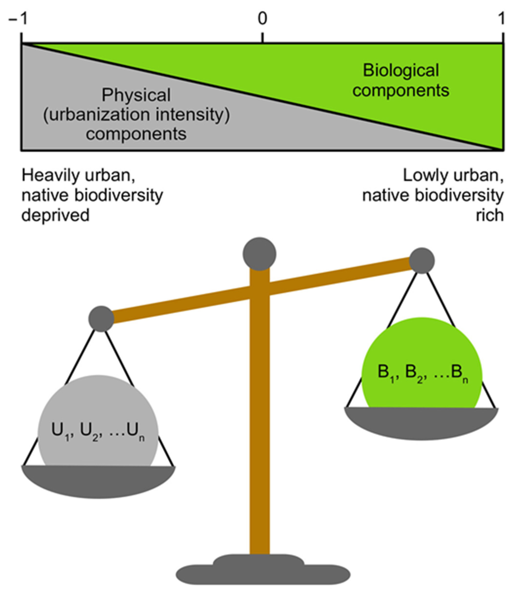
Abstract
:1. Introduction
2. Materials and Methods
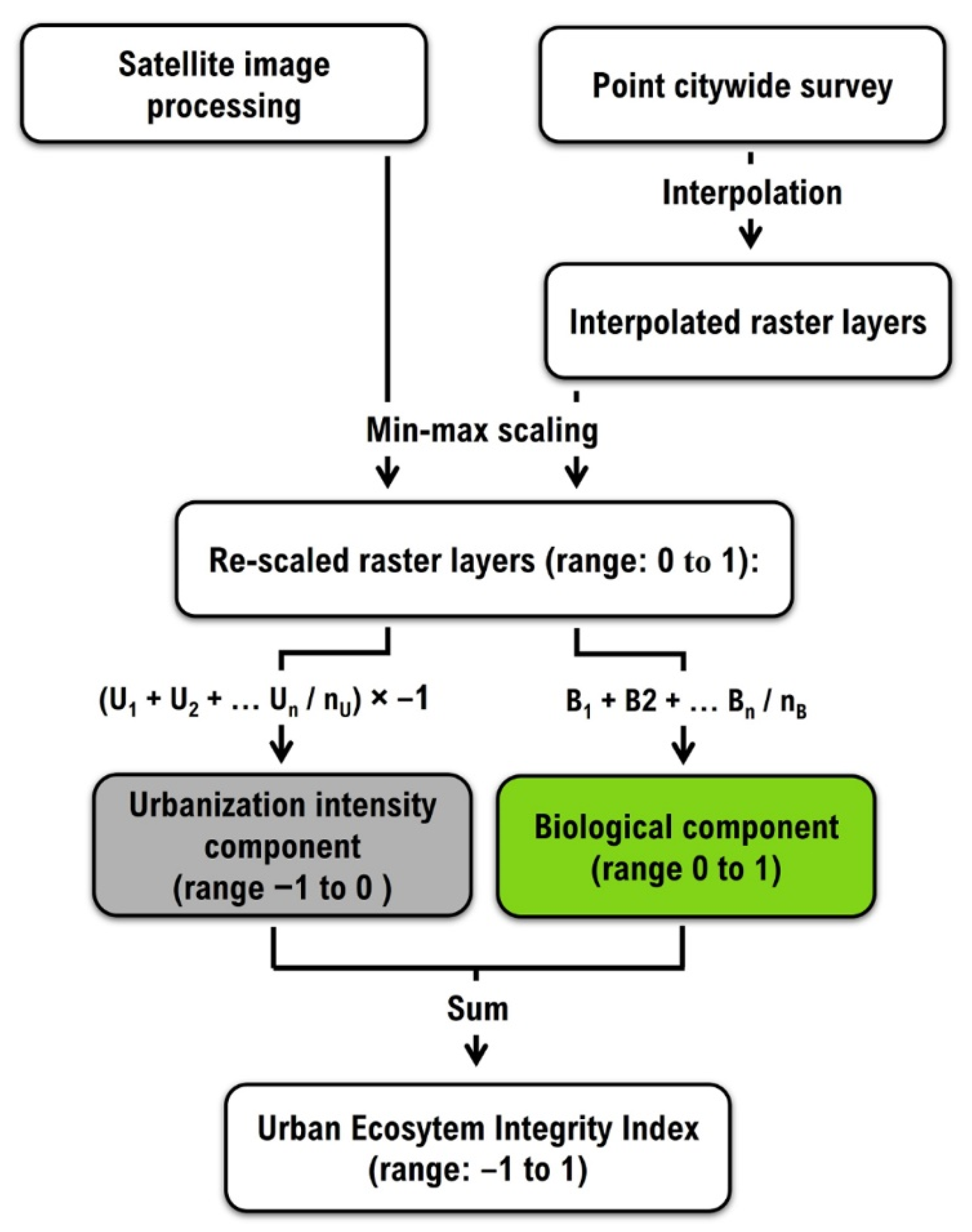
2.1. Urban Ecosystem Integrity Index
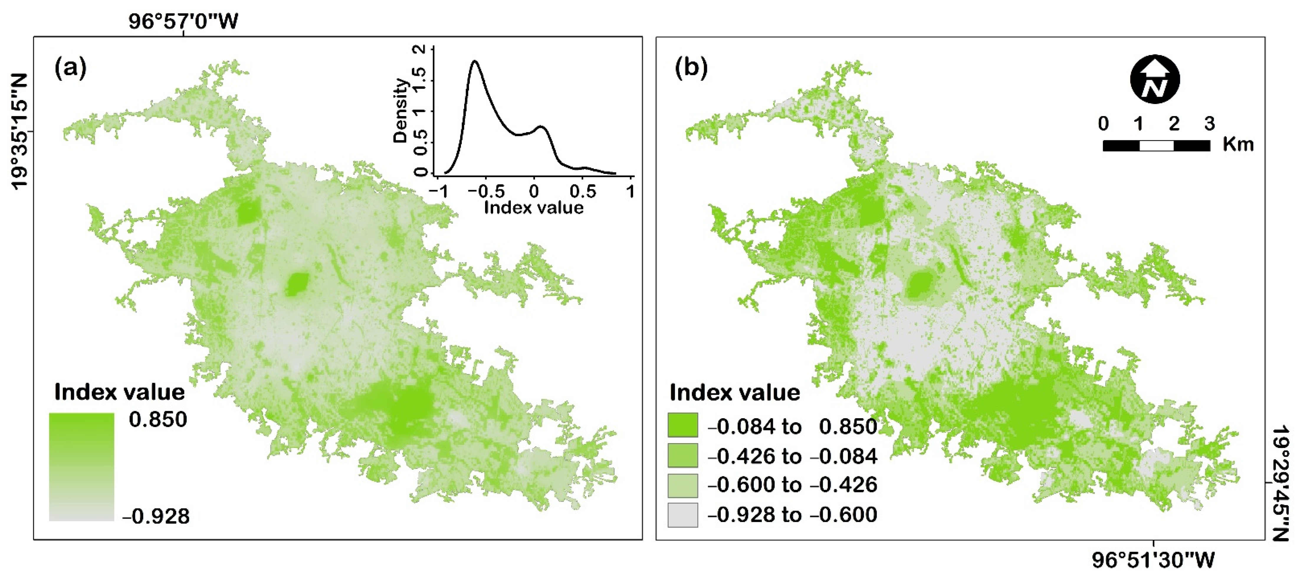
2.2. Case Study: Xalapa
2.2.1. Study Site
2.2.2. UEII for Xalapa
3. Results and Discussion
4. Conclusions
Author Contributions
Funding
Data Availability Statement
Acknowledgments
Conflicts of Interest
References
- Elmqvist, T.; Andersson, E.; McPhearson, T.; Bai, X.; Bettencourt, L.; Brondizio, E.; Colding, J.; Daily, G.; Folke, C.; Grimm, N.; et al. Urbanization in and for the Anthropocene. NPJ Urban Sustain. 2021, 1, 6. [Google Scholar] [CrossRef]
- Grimm, N.B.; Faeth, S.H.; Golubiewski, N.E.; Redman, C.L.; Wu, J.; Bai, X.; Briggs, J.M. Global change and the ecology of cities. Science 2008, 319, 756–760. [Google Scholar] [CrossRef] [PubMed] [Green Version]
- Rees, W.E. Urban ecosystems: The human dimension. Urban Ecosyst. 1997, 1, 63–75. [Google Scholar] [CrossRef]
- United Nations. World Urbanization Prospects: The 2014 Revision. Highlights; UN: New York, NY, USA, 2014. [Google Scholar]
- Cadenasso, M.L.; Pickett, S.T.A.; Schwarz, K. Spatial heterogeneity in urban ecosystems: Reconceptualizing land cover and a framework for classification. Front. Ecol. Environ. 2007, 5, 80–88. [Google Scholar] [CrossRef]
- Pickett, S.T.A.; Cadenasso, M.L.; Grove, J.M.; Nilon, C.H.; Pouyat, R.V.; Zipperer, W.C.; Costanza, R. Urban ecological systems: Linking terrestrial ecological, physical, and socioeconomic components of metropolitan areas. In Urban Ecology: An International Perspective on the Interaction between Humans and Nature; Marzluff, J.M., Shulenberger, E., Endlicher, W., Alberti, M., Bradley, G., Ryan, C., Simon, U., ZumBrunnen, C., Eds.; Springer: Boston, MA, USA, 2008; pp. 99–122. [Google Scholar]
- Wackernagel, M.; Kitzes, J.; Moran, D.; Goldfinger, S.; Thomas, M. The ecological footprint of cities and regions: Comparing resource availability with resource demand. Environ. Urban 2006, 18, 103–112. [Google Scholar] [CrossRef]
- Vlahov, D.; Galea, S. Urbanization, urbanicity, and health. J. Urban Health 2002, 79, S1–S12. [Google Scholar] [CrossRef] [Green Version]
- Batty, M. The size, scale and shape of cities. Science 2008, 319, 769–771. [Google Scholar] [CrossRef] [Green Version]
- Castells, M. La Cuestión Urbana, 14th ed.; Siglo XXI: Distrito Federal, Mexico, 1997. [Google Scholar]
- Grimm, N.B.; Grove, J.G.; Pickett, S.T.; Redman, C.L. Integrated approaches to long-term studies of urban ecological systems. BioScience 2000, 50, 571–584. [Google Scholar] [CrossRef] [Green Version]
- Rydin, Y.; Bleahu, A.; Davies, M.; Dávila, J.D.; Friel, S.; De Grandis, G.; Groce, N.; Hallal, P.C.; Hamilton, I.; Howden-Chapman, P.; et al. Shaping cities for health: Complexity and the planning of urban environments in the 21st century. Lancet 2012, 379, 2079–2108. [Google Scholar] [CrossRef] [Green Version]
- Klopp, J.M.; Petretta, D.L. The urban sustainable development goal: Indicators, complexity and the politics of measuring cities. Cities 2017, 63, 92–97. [Google Scholar] [CrossRef]
- Westfall, M.S.; De Villa, V.A. (Eds.) Urban Indicators for Managing Cities; Asian Development Bank: Manila, Philippines, 2001. [Google Scholar]
- Andreasen, J.K.; O’Neill, R.V.; Noss, R.; Slosser, N.C. Considerations for the development of a terrestrial index of ecological integrity. Ecol. Indic. 2001, 1, 21–35. [Google Scholar] [CrossRef]
- Ferreira, V.; Barreira, A.P.; Loures, L.; Antunes, D.; Panagopoulos, T. Stakeholders’ engagement on nature-based solutions: A systematic literature review. Sustainability 2020, 12, 640. [Google Scholar] [CrossRef] [Green Version]
- Kabisch, N.; Frantzeskaki, N.; Pauleit, S.; Naumann, S.; Davis, M.; Artmann, M.; Haase, D.; Knapp, S.; Korn, H.; Stadler, J.; et al. Nature-based solutions to climate change mitigation and adaptation in urban areas: Perspectives on indicators, knowledge gaps, barriers, and opportunities for action. Ecol. Soc. 2016, 21, 39. [Google Scholar] [CrossRef] [Green Version]
- Mori, K.; Christodoulou, A. Review of sustainability indices and indicators: Towards a New City Sustainability Index (CSI). Environ. Impact Assess. Rev. 2012, 32, 94–106. [Google Scholar] [CrossRef]
- Niemelä, J. Ecology of Urban Green Spaces: The way forward in answering major research questions. Landsc. Urban Plan 2014, 125, 298–303. [Google Scholar] [CrossRef]
- Chan, L.; Djoghlaf, A. Invitation to help compile an index of biodiversity in cities. Nature 2009, 460, 33. [Google Scholar] [CrossRef]
- Pierce, J.R.; Barton, M.A.; Tan, M.M.J.; Oertel, G.; Halder, M.D.; Lopez-Guijosa, P.A.; Nuttall, R. Actions, indicators, and outputs in urban biodiversity plans: A multinational analysis of city practice. PLoS ONE 2020, 15, e0235773. [Google Scholar] [CrossRef]
- Equihua Zamora, M.; García Alaniz, N.; Pérez-Maqueo, O.; Benítez Badillo, G.; Kolb, M.; Schmidt, M.; Equihua, J.; Maeda, P.; Álvarez Palacios, J.L. Integridad ecológica como indicador de la calidad ambiental. In Bioindicadores: Guardianes de Nuestro Futuro Ambiental; González Zuarth, C.A., Vallarino, A., Pérez Jiménez, J.C., Low Pfeng, A.M., Eds.; El Colegio de la Frontera Sur, Instituto Nacional de Ecología y Cambio Climático: Distrito Federal, Mexico, 2014; pp. 687–710. [Google Scholar]
- Noss, R.F. Can urban areas have ecological integrity? In Proceedings of the 4th International Urban Wildlife Symposium on Urban Wildlife Conservation, Tucson, AZ, USA, 1–5 May 1999; University of Arizona: Tucson, AZ, USA, 2004; pp. 3–8. [Google Scholar]
- Karr, J.R.; Dudley, D.R. Ecological perspective on water quality goals. Environ. Manag. 1981, 5, 55–68. [Google Scholar] [CrossRef]
- Conway, T.M.; Almas, A.D.; Coore, D. Ecosystem services, ecological integrity, and native species planting: How to balance these ideas in urban forest management? Urban For. Urban Green. 2019, 41, 1–5. [Google Scholar] [CrossRef]
- Ordóñez, C.; Duinker, P.N. Ecological integrity in urban forests. Urban Ecosyst. 2012, 15, 863–877. [Google Scholar] [CrossRef] [Green Version]
- Rohwer, Y.; Marris, E. Ecosystem integrity is neither real nor valuable. Conserv. Sci. Pract. 2021, 3, e411. [Google Scholar] [CrossRef]
- Karr, J.R.; Larson, E.R.; Chu, E.W. Ecological integrity is both real and valuable. Conserv. Sci. Pract. 2021, e583. [Google Scholar] [CrossRef]
- Shathy, S.T.; Reza, M.I.H. Sustainable cities: A proposed Environmental Integrity Index (EII) for decision making. Front. Environ. Sci. 2016, 4, 82. [Google Scholar] [CrossRef] [Green Version]
- Beyene, A.; Legesse, W.; Triest, L.; Kloos, H. Urban impact on ecological integrity of nearby rivers in developing countries: The borkena river in highland Ethiopia. Environ. Monit. Assess. 2009, 153, 461–476. [Google Scholar] [CrossRef]
- Blumetto, O.; Castagna, A.; Cardozo, G.; García, F.; Tiscornia, G.; Ruggia, A.; Scarlato, S.; Albicette, M.M.; Aguerre, V.; Albin, A. Ecosystem integrity index, an innovative environmental evaluation tool for agricultural production systems. Ecol. Indic. 2019, 101, 725–733. [Google Scholar] [CrossRef]
- Hansen, A.; Barnett, K.; Jantz, P.; Phillips, L.; Goetz, S.J.; Hansen, M.; Venter, O.; Watson, J.E.M.; Burns, P.; Atkinson, S.; et al. Global humid tropics forest structural condition and forest structural integrity maps. Sci. Data 2019, 6, 232. [Google Scholar] [CrossRef] [Green Version]
- Grantham, H.S.; Duncan, A.; Evans, T.D.; Jones, K.R.; Beyer, H.L.; Schuster, R.; Walston, J.; Ray, J.C.; Robinson, J.G.; Callow, M.; et al. Anthropogenic modification of forests means only 40% of remaining forests have high ecosystem integrity. Nat. Commun. 2020, 11, 5978. [Google Scholar] [CrossRef]
- Li, P.; Zhang, Y.; Lu, W.; Zhao, M.; Zhu, M. Identification of priority conservation areas for protected rivers based on ecosystem integrity and authenticity: A case study of the Qingzhu River, Southwest China. Sustainability 2021, 13, 323. [Google Scholar] [CrossRef]
- Hansen, A.J.; Noble, B.P.; Veneros, J.; East, A.; Goetz, S.J.; Supples, C.; Watson, J.E.M.; Jantz, P.A.; Pillay, R.; Jetz, W.; et al. Toward monitoring forest ecosystem integrity within the post-2020 global biodiversity framework. Conserv. Lett. 2021, 14, e12822. [Google Scholar] [CrossRef]
- Zelený, J.; Mercado-Bettín, D.; Müller, F. Towards the evaluation of regional ecosystem integrity using NDVI, brightness temperature and surface heterogeneity. Sci. Total Environ. 2021, 796, 148994. [Google Scholar] [CrossRef]
- Falfán, I.; Muñoz-Robles, C.A.; Bonilla-Moheno, M.; MacGregor-Fors, I. Can you really see ‘green’? assessing physical and self-reported measurements of urban greenery. Urban For. Urban Green. 2018, 36, 13–21. [Google Scholar] [CrossRef]
- So, A.; Joseph, T.V.; John, R.T.; Worsley, A.; Asare, D.S. The Data Science Workshop: A New, Interactive Approach to Learning Data Science; Packt Publishing Ltd.: Birmingham, UK, 2020. [Google Scholar]
- Moreno, C.E.; Rojas, G.S.; Pineda, E.; Escobar, F. Shortcuts for biodiversity evaluation: A review of terminology and recommendations for the use of target groups, bioindicators and surrogates. Int. J. Environ. Health 2007, 1, 71–86. [Google Scholar] [CrossRef]
- INEGI (Instituto Nacional de Estadística y Geografía) Censo de Población y Vivienda 2020. Available online: https://www.inegi.org.mx/programas/ccpv/2020/#Microdatos (accessed on 22 February 2021).
- López-Moreno, I.R. (Ed.) Ecología Urbana Aplicada a La Ciudad de Xalapa; Instituto de Ecología, A.C., Man and the Biosphere Programme—United Nations Educational, Scientific and Cultural Organization (MAB UNESCO), H. Ayuntamiento de Xalapa, Veracruz: Veracruz, Mexico, 1993. [Google Scholar]
- Castillo-Campos, G. Vegetación y Flora Del Municipio de Xalapa, Veracruz; Instituto de Ecología, A.C., Man and the Biosphere Programme—United Nations Educational, Scientific and Cultural Organization (MAB UNESCO), H, Ayuntamiento de Xalapa, Veracruz: Veracruz, Mexico, 1991. [Google Scholar]
- Capitanachi, M.C.; Amante, H.S. Las Áreas Verdes Urbanas En Xalapa, Veracruz. Catálogo de Flora Urbana; Universidad Veracruzana, Instituto de Ecología A.C.: Veracruz, Mexico, 1995; Volume 2. [Google Scholar]
- Falfán, I.; MacGregor-Fors, I. Woody Neotropical streetscapes: A case study of tree and shrub species richness and composition in Xalapa. Madera Bosques 2016, 22, 95–110. [Google Scholar] [CrossRef] [Green Version]
- González-García, F.; Straub, R.; García, J.A.L.; MacGregor-Fors, I. Birds of a neotropical green city: An up-to-date review of the avifauna of the city of Xalapa with additional unpublished records. Urban Ecosyst. 2014, 17, 991–1012. [Google Scholar] [CrossRef]
- MacGregor-Fors, I.; Avendaño-Reyes, S.; Bandala, V.M.; Chacón-Zapata, S.; Díaz-Toribio, M.H.; González-García, F.; Lorea-Hernández, F.; Martínez-Gómez, J.; Montes de Oca, E.; Montoya, L.; et al. Multi-taxonomic diversity patterns in a neotropical green city: A rapid biological assessment. Urban Ecosyst. 2015, 18, 633–647. [Google Scholar] [CrossRef]
- MacGregor-Fors, I.; Escobar, F.; Rueda-Hernández, R.; Avendaño-Reyes, S.; Baena, M.; Bandala, V.; Chacón-Zapata, S.; Guillén-Servent, A.; González-García, F.; Lorea-Hernández, F.; et al. City “green” contributions: The role of urban greenspaces as reservoirs for biodiversity. Forests 2016, 7, 146. [Google Scholar] [CrossRef]
- MacGregor-Fors, I. How to measure the urban-wildland ecotone: Redefining ‘Peri-Urban’ areas. Ecol. Res. 2010, 25, 883–887. [Google Scholar] [CrossRef]
- Lemoine-Rodríguez, R.; MacGregor-Fors, I.; Muñoz-Robles, C. Six Decades of urban green change in a Neotropical city: A case study of Xalapa, Veracruz, Mexico. Urban Ecosyst. 2019, 22, 609–618. [Google Scholar] [CrossRef]
- Chavez, P.S. Image-based atmospheric corrections—Revisited and improved. Photogramm. Eng. Remote Sens. 1996, 62, 1025–1036. [Google Scholar]
- Leutner, B.; Horning, N.; Schwalb-Willmann, J.; Hijmans, R.J. RStoolbox: Tools for Remote Sensing Data Analysis (R Package Version 0.2.6). 2019. Available online: https://github.com/bleutner/RStoolbox (accessed on 15 May 2020).
- Lemoine-Rodríguez, R.; Mas, J.-F. LSTtools: An R Package to Process Thermal Data Derived from Landsat and MODIS Images (v0.0.2). 2020. Available online: https://doi.org/10.5281/zenodo.4010732 (accessed on 18 May 2020). [CrossRef]
- USGS (United States Geological Service). Landsat 8 Data Users Handbook; USGS Earth Resources Observation and Science: Sioux Falls, SD, USA, 2019.
- Sobrino, J.A.; Jiménez-Muñoz, J.C.; Sòria, G.; Romaguera, M.; Guanter, L.; Moreno, J.; Plaza, A.; Martínez, P. Land surface emissivity retrieval from different VNIR and TIR sensors. IEEE Trans. Geosci. Remote Sens. 2008, 46, 316–327. [Google Scholar] [CrossRef]
- Morawitz, D.F.; Blewett, T.M.; Cohen, A.; Alberti, M. Using NDVI to assess vegetative land cover change in central puget sound. Environ. Monit. Assess. 2006, 114, 85–106. [Google Scholar] [CrossRef]
- MacGregor-Fors, I. De mitos a hitos urbanos: ¿Cómo hacer ecología en selvas de Asfalto. In Manual de Técnicas Para el Estudio de Fauna Nativa en Ambientes Urbanos; Zuria, I., Olvera-Ramírez, A.M., Ramírez Bastida, P., Eds.; REFAMA, Universidad Autónoma de Querétaro: Querétaro, Mexico, 2019; pp. 19–38. [Google Scholar]
- Ralph, C.J.; Geupel, G.R.; Pyle, P.; Martin, T.E.; DeSante, D.F.; Milá, B. Handbook of Field Methods for Monitoring Landbirds; U.S.D.A., Forest Service, Pacific Southwest Research Station: Albany, CA, USA, 1996; p. 41.
- POWO Plants of the World Online Kew Science. Available online: http://www.plantsoftheworldonline.org/ (accessed on 20 May 2019).
- Kennedy, H. Data in Three Dimensions: A Guide to ArcGIS 3D Analyst; Thomson Delmar Learning: Clifton Park, NY, USA, 2004. [Google Scholar]
- Longley, P.A.; Goodchild, M.F.; Maguire, D.J.; Rhind, D.W. Geographic Information Systems and Science, 2nd ed.; John Wiley & Sons: New York, NY, USA, 2005. [Google Scholar]
- R Core Team R: A Language and Environment for Statistical Computing; R Foundation for Statistical Computing: Vienna, Austria, 2020.
- QGIS Development Team. QGIS Geographic Information System; Open Source Geospatial Foundation Project; 2020; Available online: http://qgis.osgeo.org (accessed on 25 November 2021).
- Dáttilo, W.; MacGregor-Fors, I. Ant social foraging strategies along a neotropical gradient of urbanization. Sci. Rep. 2021, 11, 6119. [Google Scholar] [CrossRef] [PubMed]
- Gómez-Martínez, M.A.; Klem, D.; Rojas-Soto, O.; González-García, F.; MacGregor-Fors, I. Window strikes: Bird collisions in a neotropical green city. Urban Ecosyst. 2019, 22, 699–708. [Google Scholar] [CrossRef]
- Escobar-Ibáñez, J.F.; Rueda-Hernández, R.; MacGregor-Fors, I. The greener the better! Avian communities across a neotropical gradient of urbanization density. Front. Ecol. Evol. 2020, 8, 500791. [Google Scholar] [CrossRef]
- Ramírez Restrepo, L.; Halffter, G. Butterfly diversity in a regional urbanization mosaic in two Mexican Cities. Landsc. Urban Plan 2013, 115, 39–48. [Google Scholar] [CrossRef]
- Méndez Romero, E.A. Alteraciones Térmicas Derivadas de La Urbanización En La Ciudad de Xalapa, Veracruz. Análisis Espacial y Temporal: 1982–2015. Master’s Thesis, El Colegio de Veracruz, Xalapa, Mexico, 2017. [Google Scholar]
- Li, J.; Li, Y.; Qian, B.; Niu, L.; Zhang, W.; Cai, W.; Wu, H.; Wang, P.; Wang, C. Development and validation of a bacteria-based index of biotic integrity for assessing the ecological status of urban rivers: A case study of Qinhuai River basin in Nanjing, China. J. Environ. Manag. 2017, 196, 161–167. [Google Scholar] [CrossRef] [PubMed]
- Kim, J.-J.; Atique, U.; An, K.-G. Long-term ecological health assessment of a restored urban stream based on chemical water quality, physical habitat conditions and biological integrity. Water 2019, 11, 114. [Google Scholar] [CrossRef] [Green Version]
- Carignan, V.; Villard, M.-A. Selecting indicator species to monitor ecological integrity: A review. Environ. Monit. Assess. 2002, 78, 45–61. [Google Scholar] [CrossRef]
- Singh, R.K.; Murty, H.R.; Gupta, S.K.; Dikshit, A.K. An overview of sustainability assessment methodologies. Ecol. Indic. 2009, 9, 189–212. [Google Scholar] [CrossRef]
- Pickett, S.T.A.; Cadenasso, M.L.; Childers, D.L.; McDonnell, M.J.; Zhou, W. Evolution and future of urban ecological science: Ecology in, of, and for the city. Ecosyst. Health Sustain. 2016, 2, e01229. [Google Scholar] [CrossRef]
- McDonnell, M.J.; MacGregor-Fors, I. The Ecological Future of Cities. Science 2016, 352, 936–938. [Google Scholar] [CrossRef] [PubMed]


Publisher’s Note: MDPI stays neutral with regard to jurisdictional claims in published maps and institutional affiliations. |
© 2021 by the authors. Licensee MDPI, Basel, Switzerland. This article is an open access article distributed under the terms and conditions of the Creative Commons Attribution (CC BY) license (https://creativecommons.org/licenses/by/4.0/).
Share and Cite
MacGregor-Fors, I.; Falfán, I.; García-Arroyo, M.; Lemoine-Rodríguez, R.; Gómez-Martínez, M.A.; Marín-Gómez, O.H.; Pérez-Maqueo, O.; Equihua, M. A Novel Approach for the Assessment of Cities through Ecosystem Integrity. Land 2022, 11, 3. https://doi.org/10.3390/land11010003
MacGregor-Fors I, Falfán I, García-Arroyo M, Lemoine-Rodríguez R, Gómez-Martínez MA, Marín-Gómez OH, Pérez-Maqueo O, Equihua M. A Novel Approach for the Assessment of Cities through Ecosystem Integrity. Land. 2022; 11(1):3. https://doi.org/10.3390/land11010003
Chicago/Turabian StyleMacGregor-Fors, Ian, Ina Falfán, Michelle García-Arroyo, Richard Lemoine-Rodríguez, Miguel A. Gómez-Martínez, Oscar H. Marín-Gómez, Octavio Pérez-Maqueo, and Miguel Equihua. 2022. "A Novel Approach for the Assessment of Cities through Ecosystem Integrity" Land 11, no. 1: 3. https://doi.org/10.3390/land11010003
APA StyleMacGregor-Fors, I., Falfán, I., García-Arroyo, M., Lemoine-Rodríguez, R., Gómez-Martínez, M. A., Marín-Gómez, O. H., Pérez-Maqueo, O., & Equihua, M. (2022). A Novel Approach for the Assessment of Cities through Ecosystem Integrity. Land, 11(1), 3. https://doi.org/10.3390/land11010003