Abstract
Data relative to two soybean seasons, several irrigation scheduling treatments, including moderate and severe deficit irrigation, and rain-fed cropping were used to parameterize and assess the performance of models AquaCrop and SIMDualKc, the latter combined with the Stewart’s yield model. SIMDualKc applies the FAO56 dual crop coefficient approach for computing and partitioning evapotranspiration (ET) into actual crop transpiration (Tc act) and soil evaporation (Es), while AquaCrop uses an approach that depends on the canopy cover curve. The calibration-validations of models were performed by comparing observed and predicted soil water content (SWC) and grain yield. SIMDualKc showed good accuracy for SWC estimations, with normalized root mean square error (NRMSE) ≤ 7.6%. AquaCrop was less accurate, with NRMSE ≤ 9.2%. Differences between models regarding the water balance terms were notable, and the ET partition revealed a trend for under-estimation of Tc act by AquaCrop, mainly under severe water stress. Yield predictions with SIMDualKc-Stewart models produced NRMSE < 15% while predictions with AquaCrop resulted in NRMSE ≤ 23% due to under-estimation of Tc act, particularly for water stressed treatments. Results show the appropriateness of SIMDualKc to support irrigation scheduling and assessing impacts on yield when combined with Stewart’s model.
1. Introduction
Uruguay is characterized by a warm temperate and humid climate, where summer crops are commonly rain-fed. Due to rainfall uncertainty, supplemental irrigation is often required for achieving high yields [1]. Thus, adequate irrigation scheduling has to be considered for soybean production. Predicting soybean yield response to water is required for assessing irrigation management strategies to be adopted by farmers. Attention should be paid to the crop stages where water stress is most critical, with several studies having identified the period from flowering to grain filling as the most sensitive to water stress [2,3,4].
Crop growth and yield models are often used. The CROPGRO-Soybean model is probably the most used to simulate soybean growth and yield. It is one of the Decision Support System for Agrotechnology Transfer-Cropping System Models (DSSAT-CSM) whose features are discussed in detail by Jones et al. [5]. Because DSSAT-CSM are oriented to represent the growth and yield processes considering a variety of constraints and stresses, they are rarely used for assessing water use or for developing irrigation scheduling scenarios. However, several applications of CROPGRO-Soybean are reported [6,7,8]. The RZWQM-CROPGRO hybrid model for soybean production [6] combines the more precise approach to water and solutes dynamics of RZWQM with the accurate prediction of yield of CROPGRO-Soybean, thus, resulting in a more useful model for practical applications related to water. Another modeling approach consists of the model SoySim [9] that has been tested on several locations and different crop varieties, growth constraints, and cropping practices. Moreover, it has been compared with other models: CROPGRO-Soybean [5], Sinclair-Soybean [10], and WOFOST [11]. A recent application of SoySim to yield prediction in Brazil was reported by Cera et al. [12]. Crop growth and yield models are quite complex, require a large number of parameters, and their parameterization is generally difficult and demanding in terms of agronomic data acquisition. Therefore, these models are generally more adequate for research purposes or for yield prediction than for operational use as a support to irrigation management by the farmers, and they may be less accurate in simulating soil water dynamics and water use; however, these models, like SOYGRO, may be useful to define irrigation schedules [13].
The Food and Agriculture Organization (FAO) AquaCrop model [14], a hybrid semi-empiric and deterministic model, is aimed at both crop yield and water use simulation and has become quite popular recently, likely because it is less demanding in terms of parameterization than the models referred to above [15,16]. However, it is much more complex in parameterization than simplified approaches combining a soil water balance model and a water-yield model such as the SIMDualKc water balance model in combination with the Stewart’s water-yield model [17,18], as reported by Paredes et al. [19,20] and by Pereira et al. [21].
Applications of the Stewart’s model are often reported in literature aiming at simplifying the assessment of irrigation scheduling impacts on yields [22,23,24,25] as it has fewer parameterization requirements than the above referred crop growth and yield models. The Stewart’s model linearly relates the relative yield loss (1 − Ya/Ym) to the relative evapotranspiration (ET) deficit (1 − ETc act/ETc) through the water-yield response factor Ky, where the actual and potential yields (Ya and Ym) are produced when ET are, respectively, the actual and potential crop ET (ETc act and ETc). A modified version of the Stewart’s model, where (1 − ETc act/ETc) is replaced by the relative transpiration deficit (1 − Tc act/Tc), was successful reported for cereals [19,21] and grain legumes [20,26], with actual and potential transpiration (Tc act and Tc) computed with the water balance SIMDualKc model, which partitions daily ET in its components Tc act and soil evaporation Es.
Considering that SIMDualKc has already been calibrated and successfully used in various applications worldwide, and that AquaCrop acceptably predicted soybean yields in southern Brazil [27], the objectives of the present study consisted of: (1) parameterizing and testing the AquaCrop model for different water management treatments; (2) calibration and validation of the SIMDualKc model for the same treatments; (3) analyzing soybean water balance terms and evapotranspiration partition with both the AquaCrop and the SIMDualKc models; (4) assessing the accuracy of the AquaCrop model and the Stewart’s water-yield model combined with SIMDualKc to predict soybean yields under various water stress conditions; and (5) assessing the strengths and weaknesses of both modelling approaches for supporting irrigation management.
2. Material and Methods
2.1. Site Characterization and Description of the Experiments
Field experiments were developed during the soybean cropping seasons of 2009–2010 to 2012–2013 in an Experimental Station at Paysandú, western Uruguay (32°22′ S, 58°4′ W, and 50 m elevation). Data for 2009–2010 and 2010–2011 were incomplete, lacking adequate soil water observations that could be used for models testing or validation; nevertheless, data were appropriate for soybean yield assessments. The average annual temperature during the period 1993–2014 was 18.3 °C and the average annual precipitation was 1327 mm, but with large inter-annual variability due to impacts of the El Niño Southern Oscillation [28] and the Pacific Decadal Oscillation [29]. Local climate is warm temperate, with humid and hot summers: Cfa according to the Köppen-Geiger classification [30]. Weather daily data including maximum and minimum air temperature (°C), solar radiation (MJ·m−2·d−1), air relative humidity (%), wind speed (m·s−1), and precipitation (mm) were collected by an automatic meteorological station (Vantage Pro 2TM, Davis Instruments, Hayward, CA, USA) located near the experimental fields. These data were used to compute daily reference evapotranspiration (ETo) with the FAO Penman Monteith (FAO-PM) equation [31]. The variability of daily rainfall and ETo during the soybean crop seasons is given in Figure A1.
The soil in the experimental fields is a Eutric Cambisol, loamy in the top layer and clay loamy underneath. The total available water (TAW), which represents the difference between the water storage in the root zone at field capacity (33 kPa) and permanent wilting point (1500 kPa), is 176 mm and 144 mm for soils 1 and 2, respectively. The respective main soil hydraulic properties are presented in Table A1. The soil water content (SWC) was measured with a calibrated neutron probe (503DR HYDROPROBE, InstroTek Inc., Martinez, CA, USA). Measurements were performed every 0.10 m until a maximum depth of 1.00 m. Soil sampling was used for the upper 0.10 m layer. Plots were cropped with the soybean variety “Don Mario 5.1i RR” (maturity group V) that is of indeterminate growth and has high yield potential. Each plot was 5 m × 2 m, with five rows spaced 0.4 m. The plant density was 30 plants m−2. Cropping practices were those recommended locally by the extension services. The irrigation system consisted of pressure compensating in-line drippers spaced 0.20 m and discharging 1.5 L·h−1. Irrigations were scheduled by performing a simple daily soil water balance applied to a depth of 1.0 m using the computed ETo and the measured SWC data. The irrigation trigger was a depletion of 60% of TAW during periods when water stress was induced, and a depletion of 40% of TAW otherwise. Irrigation depths were set to refill SWC up to 90% of θFC in the periods when water stress was not allowed and up to 60% of θFC otherwise.
The following treatments were adopted:
- (a)
- FI, full irrigation, aimed at fully satisfying crop water requirements, thus to avoid water stress in all crop growth stages;
- (b)
- DIGFill, deficit irrigation during the flowering to grain filling periods;
- (c)
- DIVeg, deficit irrigation during the vegetative period;
- (d)
- DIVeg-GFill, deficit irrigation during the vegetative to the grain filling periods;
- (e)
- Rain-fed.
Water deficits were induced by withholding irrigation or precipitation using rain shelters to allow for water deficits to be induced at desired timings in the crop season. Three replications of the referred five irrigation treatments were adopted. Completely random blocks were used. To assure good crop establishment, no stress was allowed during emergence. The irrigation depths applied during both crop seasons and all irrigation treatments are presented in Table A2.
The dates of each crop growth stage as defined in FAO56 [31] and the respective cumulated growing degree days (CGDD, °C) are presented in Table A3. Measurements of the photosynthetically active radiation (PAR) were performed in the treatment FI using a ceptometer (Decagon AccuPar LP 80). Following Farahani et al. [32], these measurements were converted into canopy cover (CC) and fraction of ground cover (fc) for use with AquaCrop and SIMDualKc, respectively. The crop height (h, m) and rooting depths (Zr, m) were randomly measured, and the maximum root depth observed was 1 m. The final above ground biomass and soybean grain yield were obtained from harvesting all experimental plots, thus, three samples per irrigation treatment were used; samples were oven dried to a constant weight at 65 ± 5 °C.
2.2. Modelling
Two modelling approaches were used: (a) the SIMDualKc [33] soil water balance model that uses the FAO56 dual crop coefficient approach for partitioning crop ET and was combined with the modified Stewart’s global water-yield model [17] for yield predictions; and (b) the crop growth and yield model AquaCrop, that partitions ET based upon the canopy cover (CC).
As revised previously [34,35], the FAO56 dual crop coefficient approach (dual-Kc, [31,36]) accurately models and partitions ET as described in several studies (e.g., [37,38]) and when compared with the dual-source Shuttleworth-Wallace model [39]. The SIMDualKc model has been positively tested for actual transpiration using sap-flow measurements [40,41] and for soil evaporation using micro-lysimeters [42,43] including soybeans [26]. The SIMDualKc model computes crop evapotranspiration (ETc) under standard/potential, non-limiting conditions as
where ETo (mm) is the reference evapotranspiration, Kcb (dimensionless) is the potential basal crop coefficient that describes transpiration (Tc), and Ke (dimensionless) is the soil water evaporation coefficient that describes soil evaporation (Es). The model provides for separately computing potential transpiration Tc = Kcb ETo (mm) and soil evaporation Es = Ke ETo (mm). The actual crop ET (ETc act, mm) is computed by the model as a function of the available soil water in the root zone (ASW): when soil water extraction is smaller than the depletion fraction for no stress (p) then ETc act = ETc, otherwise ETc act < ETc and decreases with decreasing ASW. The ETc act and the Tc act are, therefore, defined as
where Ks (dimensionless) is the water stress coefficient (0–1). Ks is computed through a soil water balance applied to the entire root zone (SWB). Soil evaporation is given as
with Ke depending on the fraction of ground cover by vegetation (fc) and the SWC in the soil layer with depth Ze of 10–15 cm. Ke is computed daily through an SWB of the evaporation layer, which is characterized by the readily and total evaporable water (REW, TEW, mm); REW and TEW may be computed from the soil textural and water holding characteristics of the top-layer [31,36]. Ke is adjusted for mulches and for the fraction of soil wetted by irrigation and exposed to radiation.
The SWB of the root zone is performed by computing the soil water depletion Dr,i at the end of every day i:
where the depletion Dr,i−1 of the precedent day is i − 1 and the precipitation P, runoff RO, net irrigation depth I, capillary rise CR, deep percolation DP, and crop ETc act are in mm and refer to day i. CR was not considered because the water table was deep. RO was computed using the curve number (CN) approach [44]. DP was computed with a parametric equation [45] requiring two parameters, aD characterizing storage and bD referring to the velocity of vertical drainage, both estimated from soil physical characteristics [45].
The SIMDualKc model calibration consists of searching the model crop parameters—basal crop coefficients Kcb and depletion fraction for no stress p, soil evaporation parameters Ze, TEW and REW, runoff curve number CN, and DP parameters aD and bD—that minimize the deviations between the simulated and observed SWC values. The calibration is performed through an iterative procedure of searching the best parameter values within a reasonable range until SWC errors stabilize, as discussed by Pereira et al. [21]. This procedure is first applied to the crop parameters and, after, to the remaining parameters and, finally, to all parameters together. Validation consists of testing the model using the calibrated set of parameters with one or more sets of independent field data collected in the same or different years. However, if validation is performed in a soil with different characteristics, then parameters Ze, TEW, REW, aD, and bD have to be adjusted as described by Giménez et al. [46] for maize in Paysandú. Model calibration was performed using SWC values observed in the FI treatment in 2011–2012. The validation used all other datasets of 2011–2012 and 2012–2013.
As stated above, the SIMDualKc model was combined with a modified version of the water-yield model proposed by Stewart et al. [17] to assess the impacts of water deficits on yields. The version used in the present study assumes a linear variation of the relative yield loss with the relative crop transpiration deficit [19]:
where Ya and Ym are the actual and maximum yields (kg·ha−1) corresponding, respectively, to the seasonal Tc act and Tc (mm), and Ky is the water-yield response factor. The Ya values consist of observed dry grain. Values for Ym were obtained from maximum yields observed, further using the Wageningen method [18] and checking results against maximal yields achieved by best farmers. The resulting Ym are 6.15 and 5.22 t·ha−1, respectively, for 2011–2012 and 2012–2013. The value Ky = 1.25 was adopted from solving Equation (6) relative to Ky using all experimental data available. After knowing Ky and Ym, yield predictions were performed by solving Equation (6) in relation to Ya for all Tc act results of SIMDualKc.
The AquaCrop model is a crop growth and yield model used for a variety of field crops, including soybean, mainly aiming at yield prediction. The model is described by Raes et al. [14] and Vanuytrecht et al. [47], and its open source is described by Foster et al. [48], as well as in various papers quoted there. Tc is computed as
where CC* is the crop canopy cover (%) adjusted for micro-advective effects, and KcTr,x is the maximum standard crop transpiration coefficient (dimensionless) that corresponds to the Kcb mid parameter in FAO56 [31]. Tc act is obtained by adjusting Tc using the water stress coefficient Ks (0–1), as
Tc = CC*KcTr,x ETo
Tc act = Ks Tc
Ks in AquaCrop is, however, more complex than in FAO56 because it describes the effects of the soil water stress on various processes and the depletion fractions p are inputs of the model that, contrary to SIMDualKc, do not require calibration [14].
Soil evaporation is also obtained from CC* as
where Kex is the maximum soil evaporation coefficient (non-dimensional) and Kr is the evaporation reduction coefficient (0–1), with Kr < 1 when insufficient water is available in the top soil to respond to the evaporative demand of the atmosphere [14]. The product Kr (1 − CC*) Kex corresponds to Ke as defined in FAO56 as described above. The canopy cover (CC) is similar to fc in FAO56 but while SIMDualKc uses observed fc for adjusting Ke, in AquaCrop the CC observations are used to parameterize a CC* curve which is performed in three phases and focuses on four parameters that describe the curve: canopy cover at 90% emergence (cco), maximum canopy cover (CCx), canopy growth coefficient (CGC), and canopy decline coefficient (CDC) [14].
Es = Kr (1 − CC*) Kex ETo
The above ground dry biomass (B, t·ha−1) is estimated by the model using the water transpired by the crop throughout the season and the normalized biomass water productivity (BWP*, g·m−2). BWP* represents B produced per unit of area considering the cumulative transpiration and ETo [14]. The crop yield (Y, t·ha−1) is computed from B as
where HIo is the reference harvest index, describing the harvestable proportion of B, and fHI is an adjustment factor integrating five water stress factors [14].
Y = fHIHIo B
The model parameterization was initialized using the parameter values proposed by Raes et al. [14]. The parameterizations of the CC curves were first performed using a trial and error procedure. Once these curves were properly parameterized, the trial and error procedure was applied to search the KcTr,x value that leads to a better fit of SWC. In this search, the CN and REW values found for SIMDualKc were used. Growth and yield parameters of AquaCrop were obtained using the above-ground biomass observations. The parameters retained after parameterization using FI data of 2011–2012 were used for model testing using all data sets.
“Goodness-of-fit” indicators were used to assess the accuracy of model simulations at calibration and validation of SIMDualKc and parameterization and testing of AquaCrop. Indicators, following Legates and McCabe Jr. [49], Moriasi et al. [50], and described by Pereira et al. [21], were computed from the pairs of observed and predicted values, respectively, Oi and Pi (i = 1, 2, ..., n) with means and . The regression coefficient b0 of a regression forced to the origin relating Oi and Pi was used to verify the similarity between the simulated and observed values. The determination coefficient R2 of the ordinary least squares regression of the same variables was used to assess the dispersion of pairs of Oi and Pi values along the regression line, with large R2 indicating that a large fraction of the variance of observations was explained by the model. The root mean square error (RMSE) and the normalized root mean square error relative to the mean of observations (NRMSE) were adopted to assess modelling errors. In addition, the Nash and Sutcliff [51] modelling efficiency (EF) was adopted to express the relative magnitude of the mean square error (MSE = RMSE2) in relation to the variance of the observed data [49].
3. Results and Discussion
3.1. Soil Water Simulation and Models Calibration and Parameterization
Simulations with both models are presented in Figure 1: Figure 1a,b refer to DIVeg-GFill in 2011–2012, when a severe water deficit was applied from the vegetative growth to grain filling, a sensitive period to water stress; Figure 1c,d refer to FI in 2012–2013, where water stress was avoided; and Figure 1e,f are relative to rain-fed cropping in 2012–2013, where only a limited stress occurred during pod formation. Water stress for the rain-fed crop is smaller than for that of the DIVeg-GFill treatment because, contrarily to the latter, rainfall was not avoided during any period. Results show that both models behaved well and in a similar way, which is due to their careful calibration/parameterization.
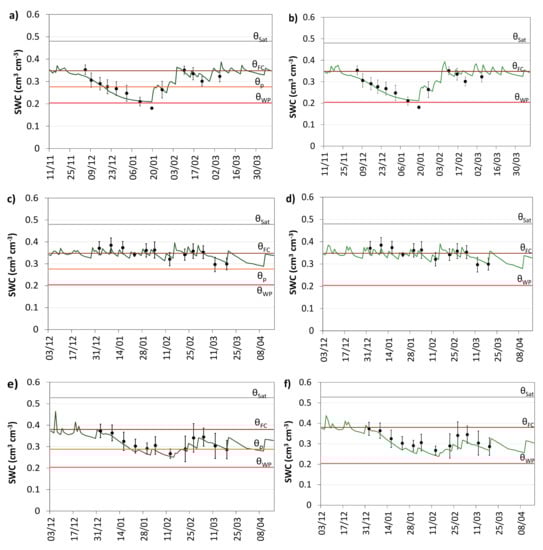
Figure 1.
Observed (●) and simulated (  ) daily average soil water content (SWC) in the soil root zone using the models SIMDualKc (left) and AquaCrop (right) for: (a,b) deficit irrigation during the vegetative to the grain filling periods (DIVeg-GFill) in 2011–2012; (c,d) full irrigation (FI) in 2012–2013; and (e,f) rain-fed in 2012–2013 (error bars indicate the standard deviation of SWC observations; θSat, θFC, θWP, and θp are, respectively, the SWC at saturation, field capacity, wilting point, and at the threshold depletion for no stress).
) daily average soil water content (SWC) in the soil root zone using the models SIMDualKc (left) and AquaCrop (right) for: (a,b) deficit irrigation during the vegetative to the grain filling periods (DIVeg-GFill) in 2011–2012; (c,d) full irrigation (FI) in 2012–2013; and (e,f) rain-fed in 2012–2013 (error bars indicate the standard deviation of SWC observations; θSat, θFC, θWP, and θp are, respectively, the SWC at saturation, field capacity, wilting point, and at the threshold depletion for no stress).
The “goodness-of-fit” indicators relative to all SWC simulations with SIMDualKc and AquaCrop (Table 1) show a better model performance when SIMDualKc is used. Regression coefficients (b0) ranged from 0.95 to 1.01 and R2 varied from 0.65 to 0.94 for SIMDualKc applications indicating that the predicted and observed values were statistically similar and a large fraction of the total variance of the observed SWC values was explained by the model. Wider but acceptable values were obtained for AquaCrop, with b0 ranging from 0.92 to 1.06 and R2 varying from 0.61 to 0.92. The estimation errors were small for SIMDualKc (RMSE < 0.025 cm3·cm−3 and NRMSE < 7.6%) and slightly larger for AquaCrop (RMSE < 0.029 cm3·cm−3 and NRMSE < 9.2%). Model efficiency was high for SIMDualKc, with EF ranging from 0.61 to 0.91, indicating that simulation errors MSE were much smaller than the variance of SWC observations. In contrast, EF values obtained for AquaCrop showed a wider range of variation, 0.16 to 0.93, indicating that MSE varied widely relative to the variance of observations. Overall, results indicate that though both models are appropriate for simulating daily SWC, SIMDualKc performed better.

Table 1.
“Goodness-of-fit” indicators of the simulation of SWC with SIMDualKc and AquaCrop.
The SIMDualKc calibrated parameters—Kcb, p, TEW, REW, Ze, CN, aD, and bD—are presented in Table 2. CN, Ze, REW, TEW, aD, and bD are the same as those previously obtained by Giménez et al. [46] for the same experimental area because they essentially depend upon the soil characteristics rather than the crop. The Kcb and p values are equal to those proposed by Allen et al. [31], Kcb ini = 0.15, Kcb mid = 1.10 and Kcb end = 0.33. Slightly lower Kcb mid values were obtained by Odhiambo and Irmak [52] and Wei et al. [26]. Kcb ini and Kcb end reported by those authors are about the same as for the current study. Calibrated Kcb mid values are also coherent to the single crop coefficients Kc mid reported by Karam et al. [3], Tabrizi et al. [53] and Payero and Irmak [54]. Thus, results relative to potential Kcb and p values confirm those proposed in FAO56 [31].
Table 2.
SIMDualKc calibrated parameters and AquaCrop conservative and calibrated parameters.
Relative to AquaCrop, the “goodness-of-fit” of CC curves for FI in both seasons have shown a slight under-estimation trend, with b0 = 0.93, but other goodness-of-fit indicators were generally high, with an R2 of 0.99 and RMSE of 6.8% and 6.4% for 2011–2012 and 2012–2013 seasons, respectively. These values are within the range of other AquaCrop applications to soybean [15,16,55]; thus, one may consider the parameterization of the CC curves in the current study adequate.
The conservative and non-conservative parameters used in AquaCrop are also presented in Table 2. The value for KcTr,x = 1.10 equals the Kcb mid calibrated with SIMDualKc (Table 2). Similar values were reported by Abi Saab et al. [15] and Paredes et al. [16]. BWP* = 14 g·m−2 equals the one reported by Abi Saab et al. [15] and Khoshravesh et al. [55]; a higher value was reported by Paredes et al. [16]. For no-stress conditions, HIo observed in both seasons averaged 0.38. That HIo value equals that reported by Paredes et al. [16]; slightly smaller values were reported by Andrade [2] and larger values by Abi Saab et al. [15] and Khoshravesh et al. [55]. Differences in BWP* and HIo values may relate to soybean varieties. Results analyzed show that parameters in Table 2 are appropriate for use in Uruguay.
3.2. Water Balance and Water Use Components
The actual ETc computed with SIMDualKc and AquaCrop were quite similar (Table 3), which agree with the results of SWC simulation discussed above. However, its partition on Tc act and Es produced different values, with AquaCrop generally giving a smaller Tc act and a larger Es. Comparing Equations (3)–(7) and Equations (4)–(9), it is apparent that differences mainly stem from procedures used to compute the actual Kcb and Ke. In fact, the daily Kcb and Kcb act curves obtained with SIMDualKc and AquaCrop are quite different (Figure 2), particularly under severe water stress (Figure 2a,b). Differences largely stem from the form of the potential Kcb curve, with SIMDualKc using the typical linear variation of Kcb for the four crop growth stages adopted in FAO56 [31], i.e., a Kcb curve defined with only three values—Kcb ini, Kcb mid, and Kcb end—(Figure 2a,c,e), while a curvilinear variation of Kcb dictated by the parameterized CC curve is adopted in AquaCrop (Figure 2b,d,f). Without a very severe stress, the variation of Kcb are somewhat similar for both models (Figure 2c,d, and Figure 2e,f) but when a severe water stress occurs, e.g., DIVeg-GFill in 2011–2012 (Figure 2b), the Kcb curve of AquaCrop is far from representing the potential Kcb defined in FAO56 [31,35] because this model does not use Kcb mid but just the maximum KcTr,x. When water stress occurs but it does not affects crop development noticeably, as is the case of the rain-fed treatment, both Figure 2e,f show a similar behavior of Kcb act until the end of February, but not afterwards, likely due to the model approach used to compute the stress coefficient Ks in AquaCrop which includes various stresses in addition to soil water deficits.
Table 3.
Simulated soil evaporation (Es), actual transpiration (Tc act), and the ratio Es/ETc act for the various crop growth stages and all different irrigation treatments of soybean when using the SIMDualKc (SIM) and AquaCrop (Aqua) models in the 2011–2012 and 2012–2013 seasons.
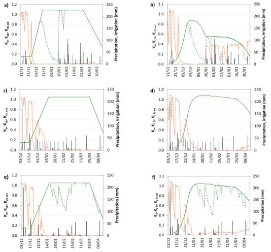
Figure 2.
Selected examples of the daily variation of the standard and actual basal crop coefficients (Kcb─ ─ and Kcb act──) and of the evaporation coefficient (Ke─ ─) computed with SIMDualKc (on left) and AquaCrop (on right) relative to the irrigation treatments DIVeg-GFill in 2011–2012 (a,b), FI in 2012–2013 (c,d), and rain-fed in 2012–2013 (e,f). Precipitation (▐) and irrigation (▐) are also depicted.
The daily variation of the Ke in all examples of Figure 2 shows a similar behavior during the initial and early vegetative crop stages, though AquaCrop shows a tendency to estimate a larger Ke. In contrast, Ke tends to be larger afterwards when water stress occurs particularly during mid-season. Differences in Ke computed by both models increase when water deficits are larger (Figure 2a,b). Differences between models are due to the fact that Ke in SIMDualKc varies with the observed fc and the daily computed depletion of the soil evaporation layer [33], while Ke in AquaCrop depends upon the fitted CC curve. Therefore, Ke tends to be higher with AquaCrop when water deficits occur. Under no stress conditions, differences are negligible (Figure 2c,d) as observed by Paredes et al. [16].
Analyzing the ET estimates and partition into Es and Tc act during the initial period (Table 3) it was observed that Es simulated by SIMDualKc represented 81% to 85% of ETc act while AquaCrop simulated a larger Es corresponding to 92% to 97% of ETc act, thus resulting in a small Tc act during this period.
Throughout the crop development stage, Es progressively decreased, as shown in Figure 2, due to the progressive decrease of the soil surface fraction exposed to solar radiation. During this period, Es/ETc act falls, in average, to 29% and 33% when computed with SIMDualKc and AquaCrop, respectively. During the mid-season, the soil is nearly fully shadowed by the crop and the energy available for evaporation drops to minimum values. Thus, Es/ETc act falls to 2% and 6% on average when computed with SIMDualKc and AquaCrop, respectively (Table 3). However, estimated Es/ETc act using AquaCrop had a very wide range, from 1% to 26%, likely due to the heavy dependency of Es on CC (Equation (7)), i.e., whenever the model simulated high impacts of water stress and reduced CC, as for DIVeg-GFill and the rain-fed treatments during 2011–2012, higher Es/ETc act values were estimated. Thus, differences between models relative to Tc act amounted to up to 40% when water stress occurred, with higher Tc act values being estimated by SIMDualKc (Table 3). During the late season, despite lower coverage of the soil due to leaf senescence, because watering events were small and infrequent, Es/ETc act increased slightly with SIMDualKc but to a higher value averaging 15% when using AquaCrop. Farahani et al. [32] also reported high Es/ETc act ratios with AquaCrop under water stress. Consequently, it could be concluded that AquaCrop tends to underestimate Tc act throughout the crop season, mainly under water deficit conditions.
Differences relative to the non-consumptive use terms, runoff, and deep percolation are notable, particularly for the 2012–2013 season (Table 4). RO and DP, whose sum equals the difference between the water input and ETc act, differ between models, with differences stemming from computational approaches as also observed by Pereira et al. [21]. The CN value used for RO computations was the same with both models but related computational processes are different [14,33], thus RO values are also different.
Table 4.
Water balance components computed with the SIMDualKc and AquaCrop models for all irrigation treatments and both crop seasons of 2011–2012 and 2012–2013.
DP values computed with SIMDualKc were generally higher, up to 171 mm, than those estimated with AquaCrop (Table 4) due to differences in the computation of DP: SIMDualKc uses a parametric function (Liu et al. 2006) whose parameters aD and bD are calibrated, as per this application. In contrast, in AquaCrop, DP is estimated using a quasi-deterministic redistribution and drainage module based on the hydraulic characteristics of the soil [14] but does not use calibrated parameters. Possible deficiencies in that DP module were referred by Pereira et al. [21] and Iqbal et al. [56], as well as Farahani et al. [32] who compared computed with field observed DP. As analyzed by several authors (e.g., [57]), AquaCrop had not been tested for severe water stress conditions yet. Results herein relative to the soil water balance components and the insufficiencies in partition of ETc act support the need for improving that model.
3.3. Yield Predictions
The available data on water use and transpiration, biomass, and yield covering four seasons, 2009–2010 to 2012–2013, were used to test the biomass and yield predictions by AquaCrop and the Stewart’s model combined with SIMDualKc (Stew-SIM). Yields of all treatments were significantly different as per an application of ANOVA (data not shown).
Yield predictions often show better results with the Stew-SIM combined approach relative to AquaCrop (Table 5). The Stew-SIM approach shows a tendency for slightly over-predicting yields (b0 = 1.04), with relative deviations between predicted and simulated yields ranging from 1% to 66% (Table 5). AquaCrop results do not show any tendency for under- or over-estimation (b0 = 0.99) but deviations vary in a wider range, from 1% to 103%. Deviations between observed and simulated yields using the Stew-SIM approach are in the range of those reported by Ma et al. [6] using the CROPGRO-Soybean and the hybrid RZWQM-CROPGRO-Soybean model, and by Banterng et al. [58] when using the CROPGRO-Soybean model.
Table 5.
Deviations between predicted and observed soybean final yield (kg·ha−1) when using the SIMDualKc-Stewart’s approach and the AquaCrop model for all observed data.
The “goodness-of-fit” indicators relative to all yield predictions with AquaCrop were poor, with RMSE = 1.01 t ha−1, NRMSE = 22.8%, and EF = −0.41. The negative EF indicates that the MSE is larger than the variance of observations, thus, modelling predictions are poor and there is no effective advantage in using this model. Nevertheless, results in the current study relative to AquaCrop applications are in the range of those reported by Mercau et al. [7] using CROPGRO-Soybean and Cera et al. [12] using SoySim. However, better results using AquaCrop for soybean were reported by Abi Saab et al. [15], Paredes et al. [16], and Battisti et al. [27] whose studies only considered small water stress levels. The above referred results are likely due to the previously discussed poor estimation of actual transpiration when water stress occurs. Katerji et al. [57] and Pereira et al. [21] also reported that AquaCrop biomass and yield predictions were poor under severe water stress because they were hampered by poor estimations of Tc act. Good predictions were, however, obtained with AquaCrop for vining pea [59], which was cultivated without water stress, thus confirming that the use of AquaCrop predictions is only recommended when severe water stress is not considered.
The “goodness-of-fit” indicators relative to yield predictions with the Stew-SIM combined approach were RMSE = 0.65 t·ha−1, NRMSE = 14.5%, and EF = 0.43, which are much better than the indicators relative to the AquaCrop predictions. These RMSE and NRMSE values are in the range of those reported for other model applications, e.g., with the CROPGRO-Soybean model [8]. However, much lower NRMSE were reported when using DSSAT CSM CROPGRO-Soybean [5] and with the hybrid RZWQM-CROPGRO model for soybean [6]. Lower RMSE values were also reported by Setiyono et al. [9] when using the SoySim model in a comparative study using the models CROPGRO-Soybean, Sinclair-Soybean, and WOFOST. Results for these models [9] resulted in a much higher RMSE than the one obtained with the combined Stew-SIM approach. Therefore, the latter is adequate to predict yields aimed at assessing impacts of alternative irrigation scheduling strategies even when a severe stress is considered.
4. Conclusions
Experimental results relative to various deficit irrigation scheduling treatments confirm that the crop growth stage from flowering to grain filling is the most sensitive to water stress. However, the highest impacts of water stress were observed when deficits were imposed from the vegetative to the grain filling period.
Both SIMDualKc and AquaCrop models were successfully calibrated and validated for soybean using SWC data relative to all treatments and two soybean seasons. The accuracy for simulating the SWC dynamics along the crop seasons was better for SIMDualKc and lower for AquaCrop mainly for the treatments subjected to severe water stress. The water balance terms resulting from the application of both models were quite different, mainly due to different procedures for computing the daily actual basal crop coefficient and the evaporation coefficient, resulting in different values of Tc act and Es. Computations of potential and actual Kcb in SIMDualKc follow the well-established FAO56 dual-Kc methodology while maximum and actual Kcb values in AquaCrop depend heavily on the fitted CC curve which only works well for non-stressed crops. Relative to Es, there are large computational differences, also due to the strong dependency of Ke on the fitted CC curve in AquaCrop, while Ke in SIMDualKc is obtained after calibration of the parameters characterizing the evaporative top soil layer and considering the observed fc fraction.
Differences between models are quite evident in terms of non-consumptive water use, RO and DP. Differences in RO, computed with the same CN, resulted from differences in the algorithms used for the calculations by the models. Relative to DP, the computation modules are very different: in AquaCrop a quasi-deterministic module is used but without calibration; on the contrary, a parametric function is used in SIMDualKc but after calibration of its parameters.
It can be concluded that the calibrated parameters of both SIMDualKc and AquaCrop may be further used for soybean in this region and that SIMDualKc performed more accurately in computing the soil water balance, mainly in estimating Tc act, thus proving to be more appropriate to support advising farmers on supplemental irrigation scheduling.
Both the AquaCrop model and the SIMDualKc-Stewart’s combined approach may be used for yield predictions. However, AquaCrop responded poorly when severe water stress was imposed, which relates to the above referred poor estimation of Tc act under those conditions. Thus, whenever the model fitting of CC is worse, the model poorly estimates Tc act and, as a consequence, biomass and yield are under-estimated. Results herein clearly identified the main weaknesses of AquaCrop, thus, the need for its further improvement for high water deficit situations. Contrarily, yield predictions with the Stew-SIM approach were good because Tc act was predicted accurately and the empirical yield response factor Ky was calibrated. Thus, that simple approach can be further used when devising supplemental irrigation strategies for soybean in Uruguay.
Based on the current study, the next step is to design supplemental irrigation strategies to cope with climate variability in line with previous studies [13,60] and to consider water productivity and economic farmers’ returns. Further research should also assess the usability of weather forecasts for supporting real time irrigation scheduling.
Acknowledgments
Thanks are due to Professor Isabel Alves for her thorough English review. Paula Paredes thanks the postdoctoral fellowship (SFRH/BPD/102478/2014) provided by the Fundação para a Ciência e a Tecnologia (FCT). The support of FCT through the research unit LEAF—Linking Landscape, Environment, Agriculture and Food (UID/AGR/04129/2013) is also acknowledged.
Author Contributions
Luis Giménez contributed for the current study by developing the field experiments and related data analysis. Paula Paredes contributed by supporting the testing of both model applications and manuscript writing. Luis S. Pereira was responsible for the theory regarding water balance, water use, and evapotranspiration and for directing manuscript writing.
Conflicts of Interest
The authors declare no conflict of interest.
Appendix A
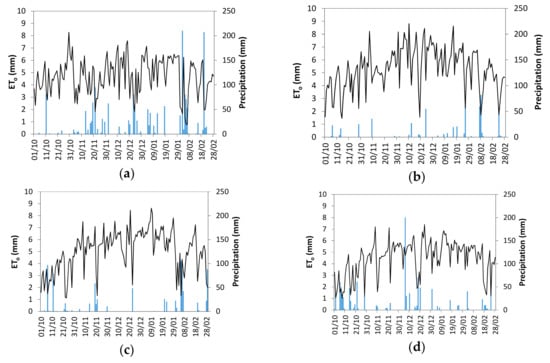
Figure A1.
Daily precipitation (│) and reference evapotranspiration (─) during the soybean seasons of (a) 2009–2010; (b) 2010–2011; (c) 2011–2012; and (d) 2012–2013, Paysandú, Uruguay.
Table A1.
Main soil hydraulic properties of the experimental site, Paysandú.
Table A1.
Main soil hydraulic properties of the experimental site, Paysandú.
| Layer Depth (m) | Soil 1 | Soil 2 | ||||||
|---|---|---|---|---|---|---|---|---|
| θsat (cm3·cm−3) | θFC (cm3·cm−3) | θWP (cm3·cm−3) | Ksat (cm·day−1) | θsat (cm3·cm−3) | θFC (cm3·cm−3) | θWP (cm3·cm−3) | Ksat (cm·day−1) | |
| 0–0.20 | 0.52 | 0.36 | 0.16 | 57.4 | 0.46 | 0.30 | 0.14 | 40.5 |
| 0.20–0.60 | 0.52 | 0.45 | 0.29 | 64.7 | 0.50 | 0.40 | 0.26 | 50.2 |
| 0.60–1.00 | 0.54 | 0.37 | 0.19 | 65.4 | 0.47 | 0.32 | 0.18 | 51.5 |
Notes: θsat, θFC,, and θWP are, respectively, the soil water content at saturation, field capacity, and wilting point; Ksat is the saturated hydraulic conductivity.
Table A2.
Crop growth stages dates and cumulated growing degree days (CGDD) for experimental seasons of 2011–2012 and 2012–2013.
Table A2.
Crop growth stages dates and cumulated growing degree days (CGDD) for experimental seasons of 2011–2012 and 2012–2013.
| Crop Growth Stages | |||||
|---|---|---|---|---|---|
| Year | Initial | Crop Development | Mid-Season | Late-Season | |
| 2011–2012 | Dates | 11 November to 29 November | 30 November to 20 December | 21 December to 4 March | 5 March to 9 April |
| CGDD (°C) * | 336 | 654 | 2015 | 2640 | |
| 2012–2013 | Dates | 3 December to 17 December | 18 December to 17 January | 18 January to 24 March | 24 March to 25 March |
| CGDD (°C) * | 363 | 759 | 1894 | 2235 | |
Note: * values obtained using a base temperature of 5 °C and a cut-off temperature of 30 °C.
Table A3.
Net irrigation depths (mm) of all irrigation treatments in soybean seasons of 2011–2012 and 2012–2013.
Table A3.
Net irrigation depths (mm) of all irrigation treatments in soybean seasons of 2011–2012 and 2012–2013.
| Irrigation Depths | Irrigation Depths | ||||||||
|---|---|---|---|---|---|---|---|---|---|
| Dates | FI | DIGFill | DIVeg | DIVeg-GFill | Dates | FI | DIGFill | DIVeg | DIVeg-GFill |
| 16 November 2011 | 36 | 36 | 36 | 36 | 5 December 2012 | 18 | 18 | 18 | 18 |
| 5 December 2011 | 36 | 36 | 29 December 2012 | 54 | 54 | 54 | 54 | ||
| 10 December 2011 | 36 | 4 January 2013 | 36 | 36 | 36 | 54 | |||
| 14 December 2011 | 36 | 9 January 2013 | 36 | 36 | 36 | ||||
| 19 December 2011 | 36 | 36 | 14 January 2013 | 36 | 36 | ||||
| 1 January 2012 | 48 | 54 | 21 January 2013 | 36 | 36 | 36 | |||
| 4 January 2012 | 36 | 28 January 2013 | 36 | 36 | |||||
| 9 January 2012 | 18 | 54 | 54 | 11 February 2013 | 36 | 54 | 54 | ||
| 20 January 2012 | 54 | 16 February 2013 | 54 | 54 | |||||
| 30 January 2012 | 36 | 36 | 15 March 2013 | 54 | 54 | ||||
| 15 February 2012 | 36 | 36 | |||||||
| Total | 354 | 216 | 162 | 90 | Total | 342 | 306 | 216 | 306 |
References
- Frank, F.C.; Viglizzo, E.F. Water use in rain-fed farming at different scales in the Pampas of Argentina. Agric. Syst. 2012, 109, 35–42. [Google Scholar] [CrossRef]
- Andrade, F.H. Analysis of growth and yield of maize, sunflower and soybean grown at Balcarce, Argentina. Field Crops Res. 1995, 41, 1–12. [Google Scholar] [CrossRef]
- Karam, F.; Masaad, R.; Sfeir, T.; Mounzer, O.; Rouphael, Y. Evapotranspiration and seed yield of field grown soybean under deficit irrigation conditions. Agric. Water Manag. 2005, 75, 226–244. [Google Scholar] [CrossRef]
- Payero, J.O.; Melvin, S.R.; Irmak, S. Response of soybean to deficit irrigation in the semi-arid environment of West-Central Nebraska. Trans. ASAE 2005, 48, 2189–2203. [Google Scholar] [CrossRef]
- Jones, J.W.; Hoogenboom, G.; Porter, C.H.; Boote, K.J.; Batchelor, W.D.; Hunt, L.A.; Wilkens, P.W.; Singh, U.; Gijsman, A.J.; Ritchie, J.T. The DSSAT cropping system model. Eur. J. Agron. 2003, 18, 235–265. [Google Scholar] [CrossRef]
- Ma, L.; Hoogenboom, G.; Ahuja, L.R.; Nielsen, D.C.; Ascough, J.C., II. Development and evaluation of the RZWQM-CROPGRO hybrid model for soybean production. Agron. J. 2005, 97, 1172–1182. [Google Scholar] [CrossRef]
- Mercau, J.L.; Dardanelli, J.L.; Collino, D.J.; Andriani, J.M.; Irigoyen, A.; Satorre, E.H. Predicting on-farm soybean yields in the pampas using CROPGRO-soybean. Field Crop. Res. 2007, 100, 200–209. [Google Scholar] [CrossRef]
- Liu, S.; Yang, J.Y.; Zhang, X.Y.; Drury, C.F.; Reynolds, W.D.; Hoogenboom, G. Modelling crop yield, soil water content and soil temperature for a soybean–maize rotation under conventional and conservation tillage systems in Northeast China. Agric. Water Manag. 2013, 123, 32–44. [Google Scholar] [CrossRef]
- Setiyono, T.D.; Cassman, K.G.; Specht, J.E.; Dobermann, A.; Weiss, A.; Yang, H.; Conley, S.P.; Robinson, A.P.; Pedersen, P.; De Bruin, J.L. Simulation of soybean growth and yield in near-optimal growth conditions. Field Crop. Res. 2010, 119, 161–174. [Google Scholar] [CrossRef]
- Sinclair, T.R. Water and nitrogen limitation in soybean grain production I. Model development. Field Crop. Res. 1986, 15, 125–141. [Google Scholar] [CrossRef]
- Boogard, H.L.; van Diepen, C.A.; Rotter, R.P.; Cabrera, J.M.C.A.; van Laar, H.H. User’s Guide for the WOFOST 7.1 Crop Growth Simulation Model and WOFOST Control Center 1.5; Technical Document 52; DLO Winand Staring Centre: Wageningen, The Netherlands, 1998. [Google Scholar]
- Cera, J.C.; Streck, N.A.; Yang, H.; Zanon, A.J.; de Paula, G.M.; Lago, I. Extending the evaluation of the SoySim model to soybean cultivars with high maturation groups. Field Crop. Res. 2017, 201, 162–174. [Google Scholar] [CrossRef]
- Gerdes, G.; Allison, B.E.; Pereira, L.S. The soybean model SOYGRO: Field calibration and evaluation of irrigation schedules. In Crop-Water-Simulation Models in Practice; Wageningen Pers: Wageningen, The Netherlands, 1995; pp. 161–173. [Google Scholar]
- Raes, D.; Steduto, P.; Hsiao, T.C.; Fereres, E. Crop Water Productivity. Calculation Procedures and Calibration Guidance, AquaCrop version 4.0; FAO: Rome, Italy, 2012. [Google Scholar]
- Abi Saab, M.T.; Albrizio, R.; Nangia, V.; Karam, F.; Rouphael, Y. Developing scenarios to assess sunflower and soybean yield under different sowing dates and water regimes in the Bekaa valley (Lebanon): Simulations with AquaCrop. Int. J. Plant Prod. 2014, 8, 457–482. [Google Scholar]
- Paredes, P.; Wei, Z.; Liu, Y.; Xu, D.; Xin, Y.; Zhang, B.; Pereira, L.S. Performance assessment of the FAO AquaCrop model for soil water, soil evaporation, biomass and yield of soybeans in north china plain. Agric. Water Manag. 2015, 152, 57–71. [Google Scholar] [CrossRef]
- Stewart, J.I.; Hagan, R.M.; Pruitt, W.O.; Danielson, R.E.; Franklin, W.T.; Hanks, R.J.; Riley, J.P.; Jackson, E.B. Optimizing Crop Production through Control of Water and Salinity Levels in the Soil; Utah Water Research Laboratory: Logan, UT, USA, 1977; p. 191. [Google Scholar]
- Doorenbos, J.; Kassam, A.H. Yield Response to Water; Irrig. Drain. Paper 33; FAO: Rome, Italy, 1979; p. 193. [Google Scholar]
- Paredes, P.; Rodrigues, G.C.; Alves, I.; Pereira, L.S. Partitioning evapotranspiration, yield prediction and economic returns of maize under various irrigation management strategies. Agric. Water Manag. 2014, 135, 27–39. [Google Scholar] [CrossRef]
- Paredes, P.; Pereira, L.S.; Rodrigues, G.C.; Botelho, N.; Torres, M.O. Using the FAO dual crop coefficient approach to model water use and productivity of processing pea (Pisum sativum L.) as influenced by irrigation strategies. Agric. Water Manag. 2017. [Google Scholar] [CrossRef]
- Pereira, L.S.; Paredes, P.; Rodrigues, G.C.; Neves, M. Modeling barley water use and evapotranspiration partitioning in two contrasting rainfall years. Assessing SIMDualKc and AquaCrop models. Agric. Water Manag. 2015, 159, 239–254. [Google Scholar] [CrossRef]
- Lorite, I.J.; Garcia-Vila, M.; Carmona, M.A.; Santos, C.; Soriano, M.A. Assessment of the irrigation advisory services’ recommendations and farmers’ irrigation management: A case study in Southern Spain. Water Resour. Manag. 2012, 26, 2397–2419. [Google Scholar] [CrossRef]
- Woli, P.; Jones, J.W.; Ingram, K.T.; Hoogenboom, G. Predicting crop yields with the agricultural reference index for drought. J. Agron. Crops Sci. 2014, 200, 163–171. [Google Scholar] [CrossRef]
- Kiymaz, S.; Ertek, A. Water use and yield of sugar beet (Beta vulgaris L.) under drip irrigation at different water regimes. Agric. Water Manag. 2015, 158, 225–234. [Google Scholar] [CrossRef]
- Gonzalez Perea, R.; Camacho Poyato, E.; Montesinos, P.; Rodriguez Diaz, J.A. Optimization of irrigation scheduling using soil water balance and genetic algorithms. Water Resour. Manag. 2016, 30, 2815–2830. [Google Scholar] [CrossRef]
- Wei, Z.; Paredes, P.; Liu, Y.; Chi, W.W.; Pereira, L.S. Modelling transpiration, soil evaporation and yield prediction of soybean in North China Plain. Agric. Water Manag. 2015, 147, 43–53. [Google Scholar] [CrossRef]
- Battisti, R.; Sentelhas, P.C.; Boote, K.J. Inter-comparison of performance of soybean crop simulation models and their ensemble in southern Brazil. Field Crop. Res. 2017, 200, 28–37. [Google Scholar] [CrossRef]
- Barreiro, M.; Tippmann, A. Atlantic modulation of El Nino influence on summertime rainfall over southeastern South America. Geophys. Res. Lett. 2008. [Google Scholar] [CrossRef]
- Kayano, M.T.; Andreoli, R.V. Relations of South American summer rainfall interannual variations with the Pacific Decadal Oscillation. Int. J. Climatol. 2007, 27, 531–540. [Google Scholar] [CrossRef]
- Kottek, M.; Grieser, J.; Beck, C.; Rudolf, B.; Rubel, F. World Map of the Koppen-Geiger climate classification updated. Meteorol. Z. 2006, 15, 259–263. [Google Scholar] [CrossRef]
- Allen, R.G.; Pereira, L.S.; Raes, D.; Smith, M. Crop Evapotranspiration—Guidelines for Computing Crop Water Requirements; FAO Irrigation and Drainage Paper 56; FAO: Rome, Italy, 1998; p. 300. [Google Scholar]
- Farahani, H.J.; Izzi, G.; Oweis, T.Y. Parameterization and evaluation of the AquaCrop model for full and deficit irrigated cotton. Agron. J. 2009, 101, 469–476. [Google Scholar] [CrossRef]
- Rosa, R.D.; Paredes, P.; Rodrigues, G.C.; Alves, I.; Fernando, R.M.; Pereira, L.S.; Allen, R.G. Implementing the dual crop coefficient approach in interactive software. 1. Background and computational strategy. Agric. Water Manag. 2012, 103, 8–24. [Google Scholar] [CrossRef]
- Kool, D.; Agam, N.; Lazarovitch, N.; Heitman, J.L.; Sauer, T.J.; Ben-Gal, A. A review of approaches for evapotranspiration partitioning. Agric. For. Meteorol. 2014, 184, 56–70. [Google Scholar] [CrossRef]
- Pereira, L.S.; Allen, R.G.; Smith, M.; Raes, D. Crop evapotranspiration estimation with FAO56: Past and future. Agric. Water Manag. 2015, 147, 4–20. [Google Scholar] [CrossRef]
- Allen, R.G.; Pereira, L.S.; Smith, M.; Raes, D.; Wright, J.L. FAO-56 Dual crop coefficient method for estimating evaporation from soil and application extensions. J. Irrig. Drain. Eng. 2005, 131, 2–13. [Google Scholar] [CrossRef]
- Cammalleri, C.; Rallo, G.; Agnese, C.; Ciraolo, G.; Minacapilli, M.; Provenzano, G. Combined use of eddy covariance and sap flow techniques for partition of ET fluxes and water stress assessment in an irrigated olive orchard. Agric. Water Manag. 2013, 120, 89–97. [Google Scholar] [CrossRef]
- Ding, R.; Kang, S.; Zhang, Y.; Hao, X.; Tong, L.; Du, T. Partitioning evapotranspiration into soil evaporation and transpiration using a modified dual crop coefficient model in irrigated maize field with ground-mulching. Agric. Water Manag. 2013, 127, 85–96. [Google Scholar] [CrossRef]
- Zhao, P.; Li, S.; Li, F.; Du, T.; Tong, L.; Kang, S. Comparison of dual crop coefficient method and Shuttleworth–Wallace model in evapotranspiration partitioning in a vineyard of northwest China. Agric. Water Manag. 2015, 160, 41–56. [Google Scholar] [CrossRef]
- Paco, T.A.; Poças, I.; Cunha, M.; Silvestre, J.C.; Santos, F.L.; Paredes, P.; Pereira, L.S. Evapotranspiration and crop coefficients for a super intensive olive orchard. An application of SIMDualKc and METRIC models using ground and satellite observations. J. Hydrol. 2014, 519, 2067–2080. [Google Scholar] [CrossRef]
- Qiu, R.; Du, T.; Kang, S.; Chen, R.; Wu, L. Assessing the SIMDualKc model for estimating evapotranspiration of hot pepper grown in a solar greenhouse in Northwest China. Agric. Syst. 2015, 138, 1–9. [Google Scholar] [CrossRef]
- Zhao, N.N.; Liu, Y.; Cai, J.B.; Rosa, R.D.; Paredes, P.; Pereira, L.S. Dual crop coefficient modelling applied to the winter wheat–summer maize crop sequence in North China Plain: Basal crop coefficients and soil evaporation component. Agric. Water Manag. 2013, 117, 93–105. [Google Scholar] [CrossRef]
- Gao, Y.; Yang, L.; Shen, X.; Li, X.; Sun, J.; Duan, A.; Wu, L. Winter wheat with subsurface drip irrigation (SDI): Crop coefficients, water-use estimates, and effects of SDI on grain yield and water use efficiency. Agric. Water Manag. 2014, 146, 1–10. [Google Scholar] [CrossRef]
- Allen, R.G.; Wright, J.L.; Pruitt, W.O.; Pereira, L.S.; Jensen, M.E. Water requirements. In Design and Operation of Farm Irrigation Systems; Hoffman, G.J., Evans, R.G., Jensen, M.E., Martin, D.L., Elliot, R.L., Eds.; American Society of Agricultural and Biological Engineers (ASABE): St. Joseph, MI, USA, 2007; pp. 208–288. [Google Scholar]
- Liu, Y.; Pereira, L.S.; Fernando, R.M. Fluxes through the bottom boundary of the root zone in silty soils: Parametric approaches to estimate groundwater contribution and percolation. Agric. Water Manag. 2006, 84, 27–40. [Google Scholar] [CrossRef]
- Gimenez, L.; Garcia-Petillo, M.; Paredes, P.; Pereira, L.S. Predicting maize transpiration, water use and productivity for developing improved supplemental irrigation schedules in western Uruguay to cope with climate variability. Water 2016. [Google Scholar] [CrossRef]
- Vanuytrecht, E.; Raes, D.; Steduto, P.; Hsiao, T.C.; Fereres, E.; Heng, L.K.; Garcia Vila, M.; Moreno, P.M. AquaCrop: FAO’s crop water productivity and yield response model. Environ. Model. Softw. 2014, 62, 351–360. [Google Scholar] [CrossRef]
- Foster, T.; Brozović, N.; Butler, A.P.; Neale, C.M.U.; Raes, D.; Steduto, P.; Fereres, E.; Hsiao, T. AquaCrop-OS: An open source version of FAO’s crop water productivity model. Agric. Water Manag. 2017, 181, 18–22. [Google Scholar] [CrossRef]
- Legates, D.; McCabe, G., Jr. Evaluating the use of goodness of fit measures in hydrologic and hydroclimatic model validation. Water Resour. Res. 1999, 35, 233–241. [Google Scholar] [CrossRef]
- Moriasi, D.N.; Arnold, J.G.; Van Liew, M.W.; Bingner, R.L.; Harmel, R.D.; Veith, T.L. Model evaluation guidelines for systematic quantification of accuracy in watershed simulations. Trans. ASABE 2007, 50, 885–900. [Google Scholar] [CrossRef]
- Nash, J.E.; Sutcliffe, J.V. River flow forecasting through conceptual models: Part 1. A discussion of principles. J. Hydrol. 1970, 10, 282–290. [Google Scholar] [CrossRef]
- Odhiambo, L.O.; Irmak, S. Evaluation of the impact of surface residue cover on single and dual crop coefficient for estimating soybean actual evapotranspiration. Agric. Water Manag. 2012, 104, 221–234. [Google Scholar] [CrossRef]
- Tabrizi, M.S.; Parsinejad, M.; Babazadeh, H. Efficacy of partial root drying technique for optimizing soybean crop production in semi-arid regions. Irrig. Drain. 2012, 61, 80–88. [Google Scholar] [CrossRef]
- Payero, J.O.; Irmak, S. Daily energy fluxes, evapotranspiration and crop coefficient of soybean. Agric. Water Manag. 2013, 129, 31–43. [Google Scholar] [CrossRef]
- Khoshravesh, M.; Mostafazadeh-Fard, B.; Heidarpour, M.; Kiani, A.R. AquaCrop model simulation under different irrigation water and nitrogen strategies. Water Sci. Technol. 2013, 67, 232–238. [Google Scholar] [CrossRef] [PubMed]
- Iqbal, M.A.; Shen, Y.; Stricevic, R.; Pei, H.; Sun, H.; Amiri, E.; Penas, A.; del Rio, S. Evaluation of the FAO AquaCrop model for winter wheat on the North China Plain under deficit irrigation from field experiment to regional yield simulation. Agric. Water Manag. 2014, 135, 61–72. [Google Scholar] [CrossRef]
- Katerji, N.; Campi, P.; Mastrorilli, M. Productivity, evapotranspiration, and water use efficiency of corn and tomato crops simulated by AquaCrop under contrasting water stress conditions in the Mediterranean region. Agric. Water Manag. 2013, 130, 14–26. [Google Scholar] [CrossRef]
- Banterng, P.; Hoogenboom, G.; Patanothai, A.; Singh, P.; Wani, S.P.; Pathak, P.; Tongpoonpol, S.; Atichart, S.; Srihaban, P.; Buranaviriyakul, S.; et al. Application of the Cropping System Model (CSM)-CROPGRO Soybean for determining optimum management strategies for soybean in tropical environments. J. Agron. Crop. Sci. 2010, 196, 231–242. [Google Scholar] [CrossRef]
- Paredes, P.; Torres, M.O. Parameterization of AquaCrop model for vining pea biomass and yield predictions and assessing impacts of irrigation strategies considering various sowing dates. Irrig. Sci. 2017, 35, 27–41. [Google Scholar] [CrossRef]
- Pereira, L.S.; Oweis, T.; Zairi, A. Irrigation management under water scarcity. Agric. Water Manag. 2002, 57, 175–206. [Google Scholar] [CrossRef]
© 2017 by the authors. Licensee MDPI, Basel, Switzerland. This article is an open access article distributed under the terms and conditions of the Creative Commons Attribution (CC BY) license (http://creativecommons.org/licenses/by/4.0/).