Enhanced Spatiotemporal Relationship-Guided Deep Learning for Water Quality Prediction

Abstract

Water quality prediction serves as a crucial basis for water environment supervision and is of great significance for water resource protection. This study utilized meteorological and water quality data from 40 monitoring stations in the Tuojiang River Basin, Sichuan Province, China. A Gated Recurrent Unit (GRU) model and a Graph Attention Network–Gated Recurrent Unit (GAT-GRU) model were constructed. Furthermore, based on the GAT-GRU framework, an Enhanced Spatio-Temporal Relation-Guided Gated Recurrent Unit (ESRG-GRU) model was developed by incorporating an explicit river network topology and a loss function that is sensitive to extreme values to strengthen spatio-temporal relationships. Water quality predictions were made for all 40 stations, and the performance of the three models was compared. The results show that, during the 7-day forecasting period, the training time of both the ESRG-GRU and the GAT-GRU models was only about 1/40 of that required for the GRU model. In terms of prediction accuracy, the average Nash–Sutcliffe efficiency (NSE) values over the 7-day forecast period were ESRG-GRU (0.7904) > GAT-GRU (0.7557) > GRU (0.6870), while the average root mean square error (RMSE) values were ESRG-GRU (0.0156) < GAT-GRU (0.0168) < GRU (0.0185). Regarding accuracy across different regions and seasons within the river basin, the ESRG-GRU model, guided by enhanced spatio-temporal deep learning, consistently outperformed both the GRU and the GAT-GRU models. This method can effectively enhance both the efficiency and accuracy of water quality prediction, thereby providing support for water environment supervision and regional water quality improvement.

1. Introduction

Water is essential for the survival and development of human society and serves as a cornerstone of ecosystems. High-quality water is crucial for safeguarding public health, protecting aquatic ecosystems, and ensuring sustainable societal development. However, major river basins worldwide are facing intensifying pollution pressures due to industrialization, urbanization, and climate change [1,2]. Water pollution has already exacerbated water scarcity in more than 2000 sub-basins globally, and it is projected that by 2050, an additional 3 billion people could be living under water-scarce conditions [3]. Due to water pollution issues, the South China region is also confronted with the challenge of seasonal water scarcity [4]. Against this backdrop of escalating global water pollution and persistent water scarcity, the importance of water quality prediction has become increasingly evident. Effective water quality forecasting provides decision-makers with valuable references for water resource allocation and pollution control strategies, while also allowing time to implement measures that can mitigate adverse changes in water quality.

Due to their ability to learn highly complex functional relationships [5], deep learning algorithms can effectively model water quality time-series data characterized by nonlinearity, dynamics, and non-stationarity [6]. This allows them to capture intricate nonlinear interactions between water quality variables and their driving factors, leading to high prediction accuracy and demonstrating significant potential for improving global water quality management [7,8]. Currently, deep learning models are widely favored in the field of water quality prediction [9]. Among them, Recurrent Neural Networks (RNNs) are commonly used for water quality time-series forecasting owing to their regression capabilities and proficiency in handling sequential data [7,10,11,12]. Long Short-Term Memory (LSTM), a variant of RNN, effectively mitigates the gradient explosion problem inherent in standard RNNs and is therefore increasingly preferred in water quality prediction studies [10,13,14,15,16]. Another RNN variant, the Gated Recurrent Unit (GRU), simplifies the LSTM structure while overcoming the vanishing gradient problem, and has seen growing application in water quality prediction in recent years [16,17,18,19,20]. Convolutional Neural Networks (CNNs), widely employed for image recognition and classification through feature-relationship extraction [21], have also been integrated with RNNs and their variants to enhance predictive performance [9,22,23,24]. Moreover, attention mechanisms have been incorporated into these models to further improve prediction accuracy [25,26,27]. Nevertheless, most existing studies primarily focus on modeling temporal features of water quality sequences, often neglecting the spatial variability within river networks arising from complex runoff mechanisms. They also rarely account for spatial connectivity between monitoring sites or physical attributes such as river reach length, making it difficult to achieve truly collaborative spatiotemporal prediction.

The primary challenges in water quality prediction involve addressing the long-term dependencies in water quality time-series data and the spatial correlations among upstream and downstream monitoring sites [28]. To overcome the current limitation of deep learning models that often neglect both spatial and temporal features, some studies have adopted hybrid approaches using Convolutional Neural Networks (CNNs) to extract spatial features, which are then combined with temporal features to improve prediction accuracy [29]. However, spatial relationships between actual monitoring sites are not limited to Euclidean distances. Describing interactions between sites using simple pixel adjacency methods may even introduce errors during modeling [30]. In recent years, researchers have begun integrating Graph Neural Networks (GNNs) into deep learning frameworks for water quality modeling [30,31]. The incorporation of GNNs enables models to capture non-Euclidean spatial dependencies [28], which better reflect the topological relationships of upstream and downstream nodes in river networks, thereby enhancing the accuracy of water quality predictions. Several scholars have utilized Graph Attention Networks (GAT) combined with GRU models to predict hydrological and water quality processes in river basins [32,33], achieving promising results. However, most studies rely on static, undirected graphs based purely on distance or fully connected structures to define inter-station relationships [32,33,34]. This approach overlooks the fundamental physical principle of unidirectional and decay-driven pollutant transport in water bodies, which may lead the model to learn spurious correlations that contradict actual hydrological processes. Developing deep learning models based on real river network topology and hydrological connectivity, while incorporating spatiotemporal features for water quality prediction, is therefore of great significance for improving both model interpretability and forecasting accuracy.

This study focuses on the Tuojiang River Basin in Sichuan Province as the research area. Using a Gated Recurrent Unit (GRU) model as the baseline, a Graph Attention Network–Gated Recurrent Unit (GAT-GRU) model is constructed by incorporating graph attention mechanisms. Furthermore, an Enhanced Spatiotemporal Relationship-Guided Gated Recurrent Unit (ESRG-GRU) model is developed based on the GAT-GRU framework. These models are applied to predict water quality at 40 key monitoring sites across the basin, providing a methodological reference for long-term, multi-site water quality forecasting and early warning.

2. Materials and Methods

2.1. Study Area

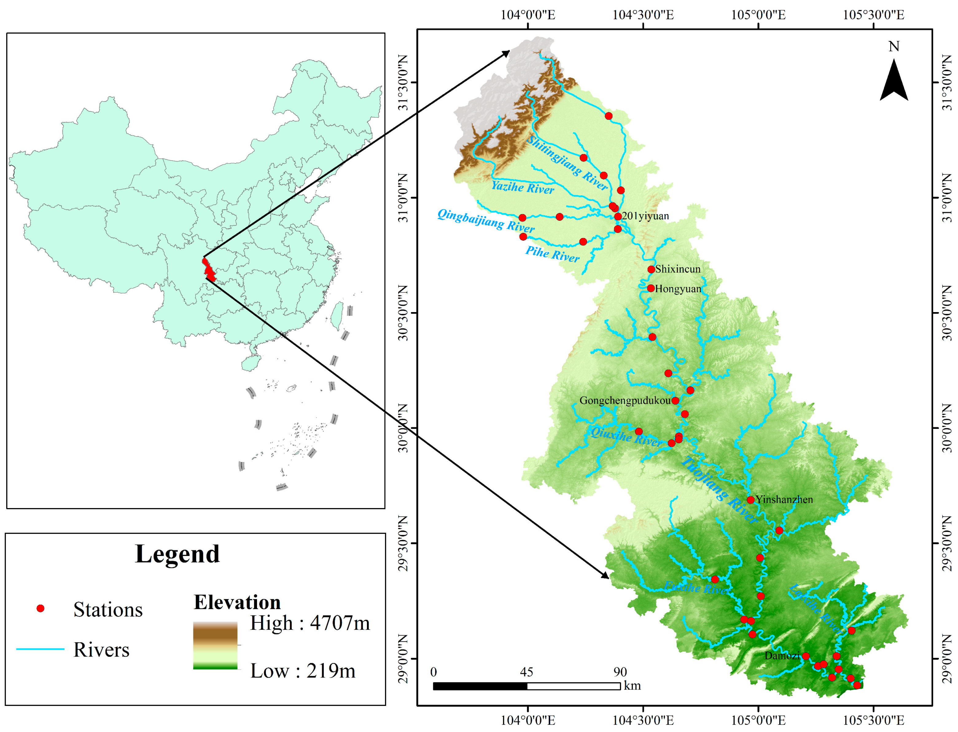
The study area is located within the Tuojiang River Basin in Sichuan Province, China, spanning approximately 28°49′ N to 31°43′ N and 103°40′ E to 105°40′ E. The basin covers an area of about 25,800 km² (shown in Figure 1). The Tuojiang River originates from the southern slope of Jiuding Mountain in the middle section of the Longmen Mountains. It flows north-to-south, passing through multiple prefecture-level cities in Sichuan, including Chengdu, Deyang, Meishan, Neijiang, Yibin, Ziyang, and Zigong, before eventually joining the Yangtze River in Luzhou. The main stream extends over 600 km and is fed by several tributaries, such as the Yazihe River, Pihe River, Qingbaijiang River, Qiuxihe River, Fuxihe River, and Laixihe River. Topographically, the basin is higher in the north and lower in the east, featuring plains and mountains in the north and low mountains and hills in the south. The region experiences a subtropical humid monsoon climate, with average annual precipitation exceeding 1000 mm, concentrated mainly between June and September.

As the most densely populated and economically dynamic region in Sichuan Province, the Tuojiang River Basin contributes 30.8% of the province’s total economic output and is home to 26.2% of its population [35]. However, rapid industrialization and urbanization have subjected the basin to multiple pollution pressures, including industrial discharge, municipal wastewater, and agricultural runoff. Among these, total phosphorus (TP) pollution constitutes a particularly serious threat to water quality [36].

2.2. Methods

2.2.1. Principle of Models

• GRU Model

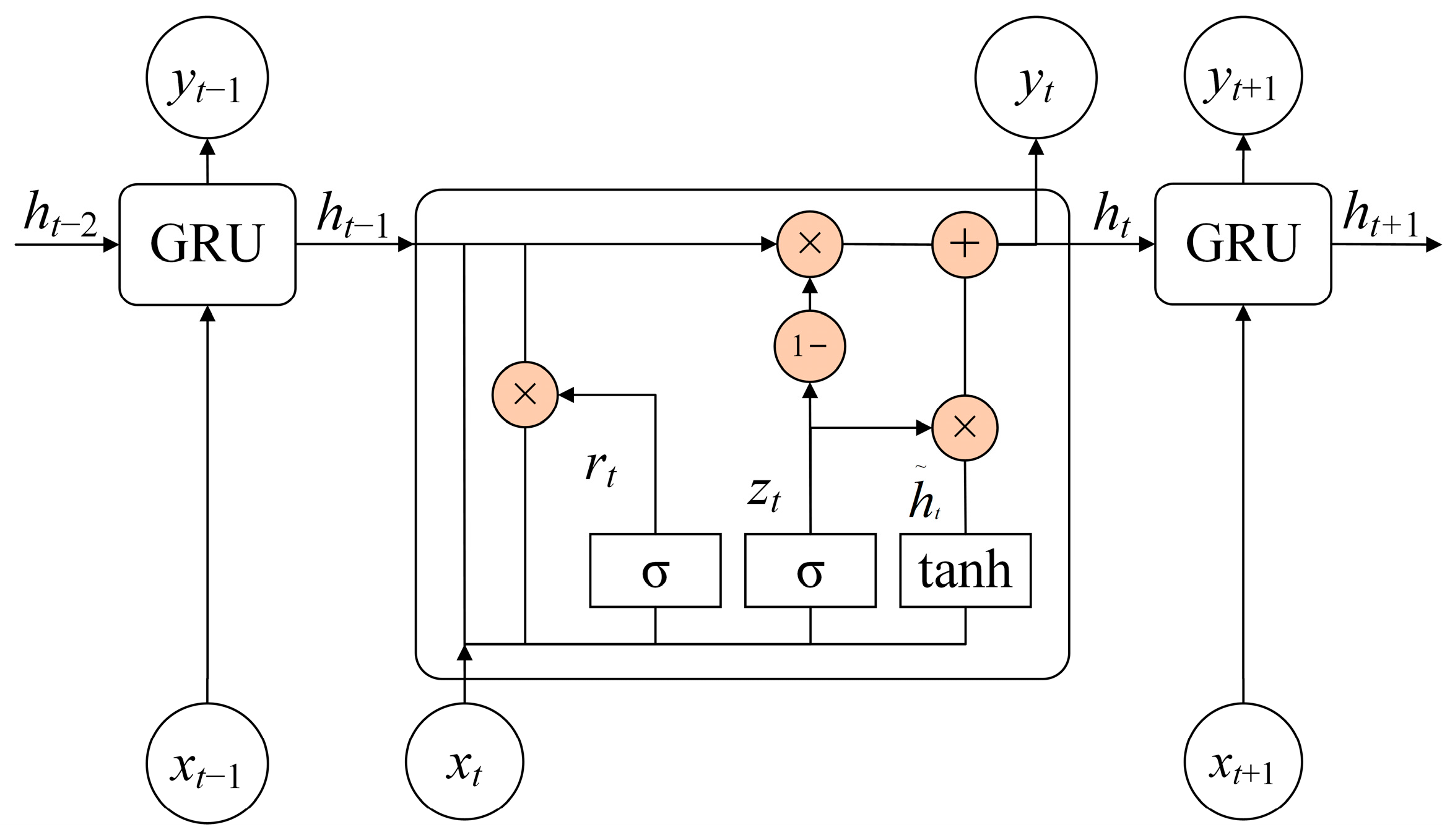
GRU is an optimized variant of the traditional RNN, designed primarily to address the common issues of gradient explosion and vanishing gradients in long sequence processing [37,38]. Compared with the three-gate structure of Long Short-Term Memory (LSTM), GRU reduces the number of gates and model parameters, resulting in higher computational efficiency. This makes it particularly suitable for sequence prediction or analysis tasks with high real-time requirements [39]. The structure of the GRU model is shown in Figure 2.

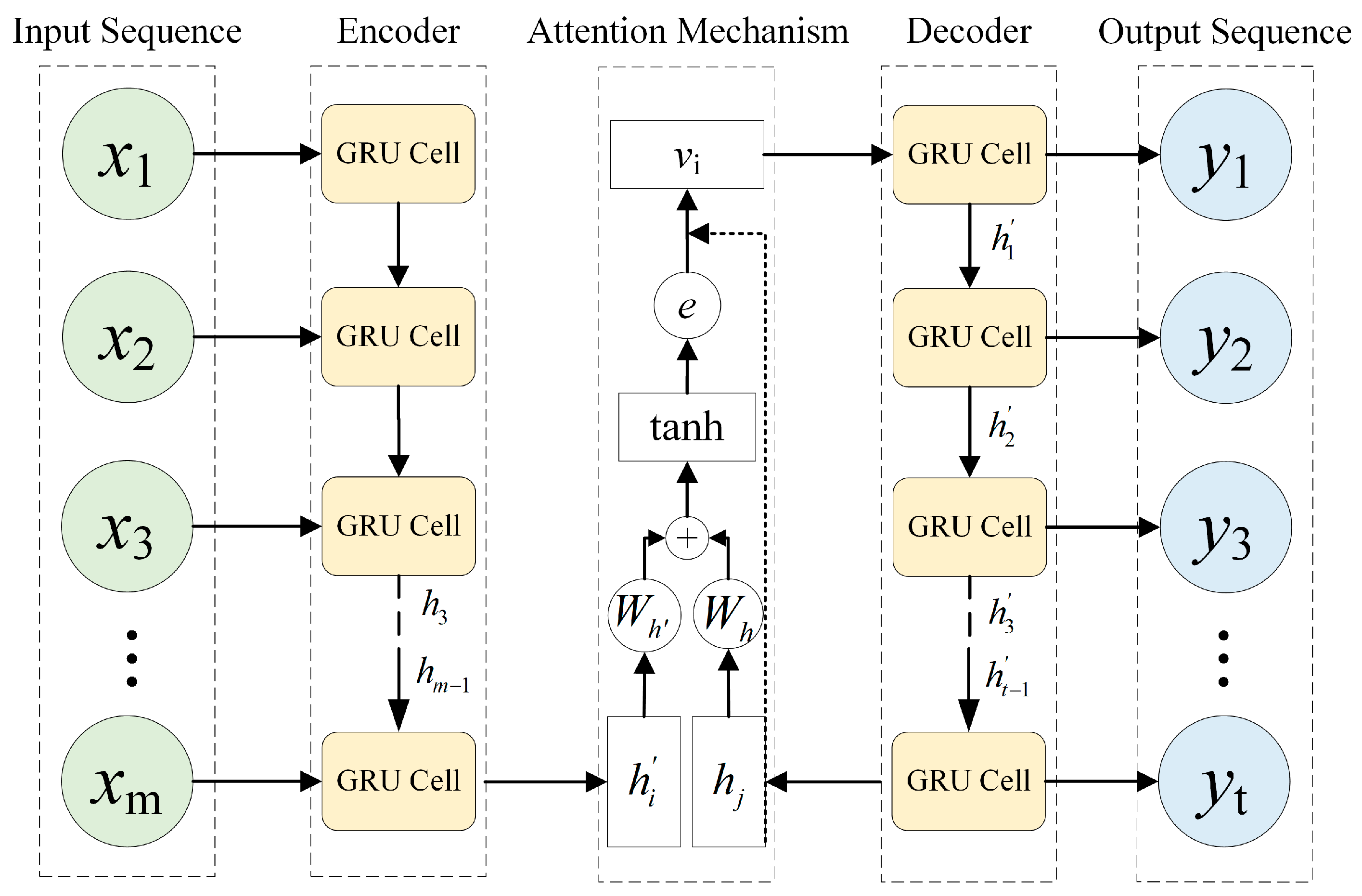
When applying the GRU model to water quality time-series prediction, the task essentially involves multi-step ahead forecasting. Changes in water quality indicators often exhibit strong long-term dependencies and non-stationary characteristics. Predicting over long sequences may lead to the loss of key temporal features, especially making it difficult to capture the coupling relationship between sudden local fluctuations and long-term gradual trends [39]. To address these issues, this study adopts an encoder–decoder framework based on GRU and incorporates an attention mechanism. Through a dynamic weight allocation strategy, the decoder adaptively focuses on the most relevant time steps of the input sequence at each prediction step, as illustrated in Figure 3.

2.

GAT-GRU Model

Graph Neural Networks (GNNs) have emerged as a pivotal method for spatiotemporal prediction due to their capacity to effectively model high-order dependencies among nodes in graph-structured data [40]. To address the need for modeling dynamic hydrological connectivity among river monitoring sites, this study constructs a GAT-GRU model as the foundational framework. The model adopts an encoder–decoder architecture, integrating Graph Attention Network (GAT) with GRU, with the aim of simultaneously capturing the spatial topological relationships and temporal evolution patterns of the river network.

(1)

GAT Layer

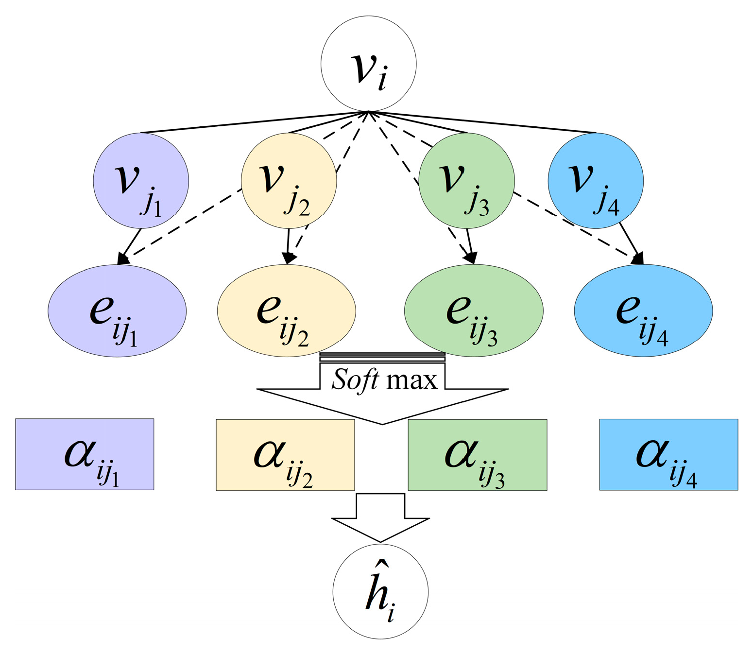
The GAT layer enables adaptive feature extraction from graph-structured data by dynamically allocating interaction weights between nodes [41,42]. Unlike traditional Graph Convolutional Networks that rely on fixed-weight convolution, GAT introduces an adaptive attention mechanism, which assigns aggregation weights to neighboring nodes through masked self-attention [43]. As illustrated in Figure 4 and Equation (2), the attention coefficient $e_{ij}$ is computed only for nodes $j\in {\mathbb{N}}_i$, where ${\mathbb{N}}_i$ denotes the neighborhood of node $v_i$ in the graph. To eliminate scale variations among the weight coefficients of different nodes, the $soft\mathrm{m}\mathrm{a}\mathrm{x}$ function is applied to normalize the coefficients within the neighborhood (Equation (2)), ensuring they satisfy the properties of a probability distribution. Finally, the output feature ${\widehat{h}}_i$ of node $v_i$ is generated by aggregating the information from its neighbors in a weighted manner, as shown in Equation (3).

$$e_{ij}=a\left(W{x}_i,W{x}_j\right)$$

(1)

$${\alpha }_{ij}=soft{\max }_j(e_{ij})={\displaystyle \frac{\exp (e_{ij})}{{\sum }_{k\in {\mathbb{N}}_i}\exp (e_{ik})}}$$

(2)

$${\widehat{h}}_i=\sigma (\sum _{j\in {\mathbb{N}}_i}{\alpha }_{ij}W{x}_j)$$

(3)

Here, $a$ denotes the shared attention mechanism; $e_{ij}$ represents the importance of node $v_j$’s features to node $v_i$; ${\alpha }_{ij}$ denotes the normalized attention weight from node $v_j$ to node $v_i$; and $a\in {\mathbb{R}}^{2F^{\prime }}$ is a learnable weight vector.

(2)

GAT-GRU Model Architecture

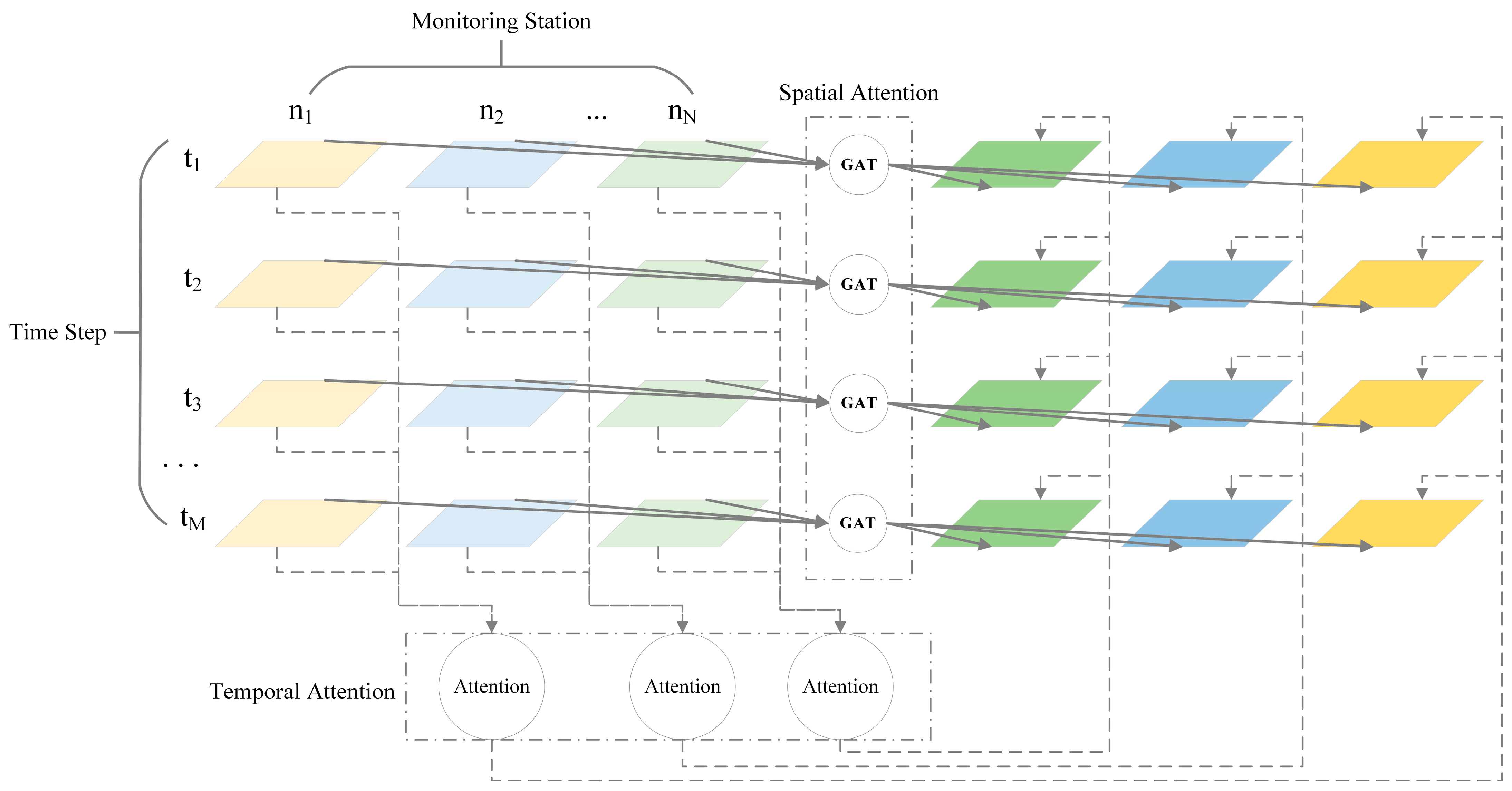
The overall workflow of the GAT-GRU model consists of three core stages, as illustrated in Figure 5. The encoder, composed of multiple GRU layers, is used to extract temporal dynamic features from the input sequence $X^{\prime }$. After dimension adjustment, the input data is fed into the GRUs to capture long-term historical dependencies, generating a hidden state sequence $H_e$. The spatio-temporal attention module enhances features through a cascaded spatial–temporal attention mechanism: the spatial attention layer is based on GAT and uses an adjacency matrix to constrain the interaction range between nodes. The aggregated spatial features S are then passed to the temporal attention layer, which employs a Query–Key–Value mechanism to focus on key historical time steps. Through weighted summation, the final spatio-temporal contextual features $C$ are obtained and serve as the input to the decoder. The decoder adopts a GRU structure symmetric to the encoder. Its initial input is the first time step of the spatio-temporal contextual features $C$. Forward propagation is then performed through the GRUs (as shown in Equation (4)), computing the output for each time step. Finally, the output is passed through a fully connected layer to produce the final prediction result.

$$h_t=GRU(x_t,h_{t-1})$$

(4)

3.

ESRG-GRU Model

While the architectures of the aforementioned foundational deep learning models, particularly the GAT-GRU model, already possess basic spatiotemporal modeling capabilities, their embedding of the physical mechanisms within hydrological systems remains insufficient. To address this limitation, this study proposes the Enhanced Spatiotemporal-Relationship-Guided Gated Recurrent Unit (ESRG-GRU). This model aims to solve two core issues: first, resolving the “black-box” weight allocation problem in the spatial dimension through explicit river network topology modeling; and second, mitigating the underestimation of peak values in the temporal dimension caused by data non-stationarity through an extremum-sensitive loss function.

(1)

Physically Constrained Spatial Modeling

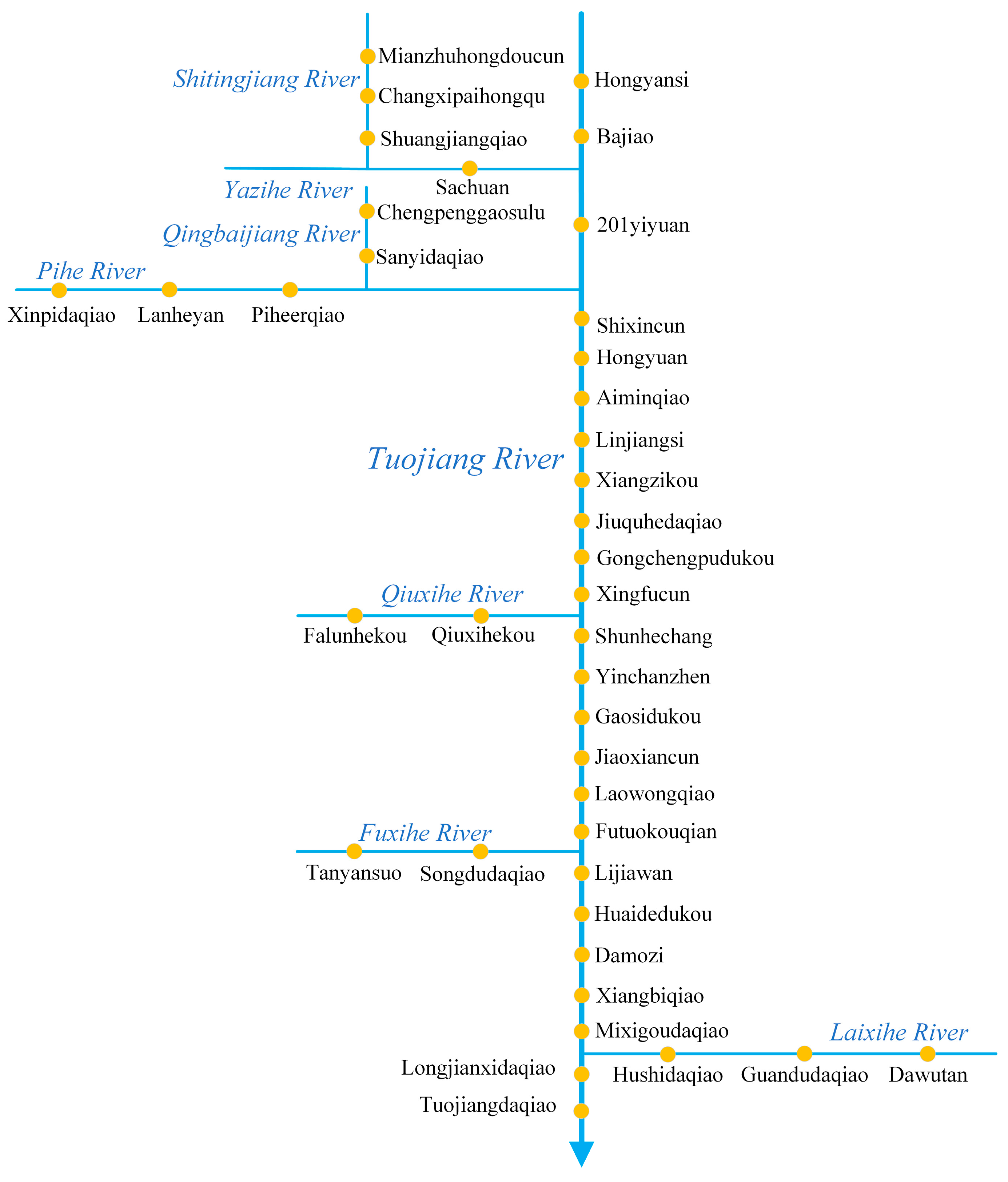
Traditional data-driven models often overlook the physical connectivity and lag effects of water flow. Building upon the GAT-GRU model structure, the ESRG-GRU model explicitly incorporates the hydrological physical attributes of the river network by reconstructing the adjacency matrix and refining the attention mechanism. A digital elevation model (DEM) was employed to delineate basin-wide flow directions using the D8 algorithm [44], thereby constructing a directed and weighted adjacency matrix that represents actual hydrological processes. Based on the coordinates of the monitoring stations, the upstream-downstream relationships between sites were established. As shown in Figure 6, the river reach length between stations is marked based on statistically derived river reach lengths. Finally, the directional connections and river reach lengths between all stations are summarized in an adjacency matrix denoted as $A\in \{0,dis{\}}^{N\times N}$. If vertices $v_i,v_j\in A$ and $(v_i,v_j)\in E$, then $A_{ij}$ is assigned the river reach length $dis$; otherwise, it is set to 0. This formulation leverages the latent physical information of cross-site transport.

Building upon the GAT, a similarity weighting mechanism based on river reach length is introduced. Attention weights are constrained using a logarithmic distance decay, which preserves potential correlations between distant stations while suppressing interference from spatially proximal but hydrologically unrelated nodes (e.g., those belonging to different tributaries) through a masking mechanism. This approach enables interpretable extraction of spatial features. The calculation formula is as follows:

$${e^{\prime }}_{ij}={\displaystyle \frac{1}{1+\log (1+dis)}}$$

(5)

(2)

Extremum-Aware Temporal Optimization

Water quality time series often exhibit significant non-stationarity and right-skewed distribution characteristics (e.g., concentration surges caused by storms or pollutant discharges). Conventional loss functions such as Mean Squared Error (MSE), which assume normally distributed errors, tend to smooth out extremes, leading to systematic underestimation of sudden pollution events. To address this, the present study designs a hybrid loss function ${Loss}_{total}$, which combines the Nash–Sutcliffe Efficiency (NSE) coefficient with an extremum loss term (Exloss) [45], as shown in Equation (6). The NSE is adopted as the base loss term to evaluate the model’s ability to simulate the overall trend of the hydrological process (Equation (7)). An Exloss term derived from generalized extreme value theory is introduced to apply asymmetric penalties according to the skewness of the data distribution (Equations (8) and (9)). Specifically, the model adaptively identifies extreme regions based on dynamic quantiles of the input data (upper quantile 80%, lower quantile 20%). For target values exceeding these thresholds, an asymmetric penalty factor is applied: when the model underestimates a high-concentration extreme, a high penalty weight ${\lambda }_{up}$ is imposed; when it overestimates an extreme, a lower penalty weight ${\lambda }_{down}$ is applied. Through this asymmetric dynamic adjustment, the model is forced to maintain balanced loss expectations in high-value intervals, thereby improving its ability to capture water pollution events.

$${Loss}_{total}={Loss}_{NSE}+{Loss}_{Exloss}$$

(6)

$$Los{s}_{NSE}={\displaystyle \frac{{\sum (Y-\widehat{Y})}^2}{{\sum (Y-\stackrel{\text{-}}{Y})}^2}}$$

(7)

$$Los{s}_{Ex}={\displaystyle \frac{L_{up}+L_{down}}{1-u{p}_{th}+dow{n}_{th}}}$$

(8)

$$L_{up,down}={\lambda }_{up,down}\mathrm{R}\mathrm{e}LU\left(ReLU\right(Y,Q_{up,down}\left(Y\right))-\mathrm{R}\mathrm{e}LU(\widehat{Y},Q_{up,down}\left(\widehat{Y}\right)\left)\right)$$

(9)

In the formulation, $Y$ and $\widehat{Y}$ denote the observed and predicted values, respectively; $\stackrel{\text{-}}{Y}$ is the mean of the observed values; the $\mathrm{R}\mathrm{e}LU$ activation ensures that penalties are applied only when the prediction error is positive, avoiding unnecessary optimization of negative errors; $Q_{up}$ and $Q_{down}$ represent the upper (80%) and lower (20%) quantile calculations, respectively; $u{p}_{th}$ and $dow{n}_{th}$ are the corresponding quantile ratios; and $1-u{p}_{th}+dow{n}_{th}$ serves as a normalization factor to ensure the loss is independent of the chosen quantile proportions.

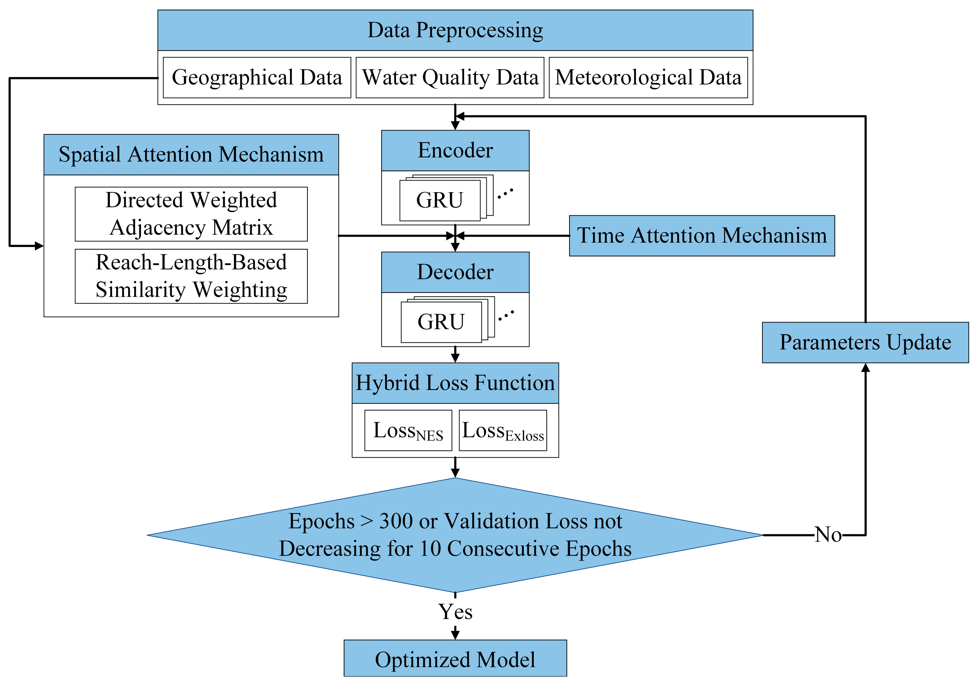
The training workflow of the ESRG-GRU model is illustrated in Figure 7. Preprocessed geographic data are used to construct the directed weighted adjacency matrix for the spatial attention mechanism and the similarity weights based on river-reach lengths, while the preprocessed water quality and meteorological data serve as multi-dimensional feature inputs to the model. The training procedure is as follows: the multi-dimensional features first undergo high-level feature extraction and fusion through an encoder composed of multiple GRU layers. The encoded features are then aggregated under the guidance of an improved spatial attention mechanism. Subsequently, a temporal attention mechanism further processes the aggregated spatial features via a Query-Key-Value mechanism to focus on key historical time steps. Finally, a weighted summation yields the spatiotemporal contextual features. These features are fed into a decoder that mirrors the GRU structure of the encoder, which then computes and outputs the water quality prediction sequence for future time steps. During the training phase, after each epoch, the value of the hybrid loss function between the model predictions and the true values is computed and recorded. Training stops when either the preset maximum number of epochs is reached or the validation loss fails to decrease for 10 consecutive epochs, at which point the trained model is obtained; otherwise, parameters are updated and the above steps continue.

2.2.2. Model Comparative Evaluation Methods

• Model Efficiency Evaluation Methods

To evaluate model efficiency, we compared the total training times of the GRU, GAT-GRU, and ESRG-GRU models under identical hardware configurations. All three models were trained on the same dataset comprising 40 monitoring stations, and their respective training durations were recorded to assess relative computational efficiency.

2.

Model Accuracy Comparative Evaluation Methods

Model accuracy was evaluated using two widely adopted metrics: the Nash–Sutcliffe Efficiency (NSE) [46], commonly applied in hydrological model goodness-of-fit assessment, and the Root Mean Square Error (RMSE) [47], a standard statistical measure used in meteorological, air-quality, and climate studies. The NSE quantifies how well a model reproduces the overall shape of a time series by comparing the mean squared error of predictions to the variance of the observations. Its value ranges from (−∞,1], with values closer to 1 indicating higher model accuracy, as shown in Equation (10). According to established interpretation guidelines [48], an NSE ≤ 0.5 is considered unsatisfactory, 0.5 < NSE < 0.6 is satisfactory, 0.6 ≤ NSE ≤ 0.8 is good, and NSE > 0.8 is very good. The RMSE is derived by taking the square root of the arithmetic mean of the squared errors (Equation (11)). Its value lies within [0, +∞), and values closer to 0 indicate smaller deviations between predicted and observed values, reflecting higher model precision.

$$NSE=1-{\displaystyle \frac{{\sum }_{i=1}^n(y_i-{\widehat{y}}_i{)}^2}{{\sum }_{i=1}^n(y_i-\stackrel{\text{-}}{y}{)}^2}}$$

(10)

$$RMSE=\sqrt{{\displaystyle \frac{1}{n}}\sum _{i=1}^n(y_i-{\widehat{y}}_i{)}^2}$$

(11)

In the equations, $n$ denotes the number of samples, $y_i$ is the observed value, ${\widehat{y}}_i$ is the predicted value, and $\stackrel{\text{-}}{y}$ is the mean of the observed values.

3. Results and Discussion

3.1. Model Construction and Training

3.1.1. Data Preprocessing

The geographic coordinates of the water quality station locations and the digital elevation model (DEM) data were standardized to the WGS 1984 datum with the UTM Zone 47 N projected coordinate system using tools from the GDAL library in Python. Subsequently, the DEM data were processed for hydrological analysis: pits were filled, a flow direction matrix was computed, and flow accumulation was calculated. A threshold of flow accumulation > 3000 was applied to extract the river network. Based on the station distribution and the river flow direction, the hydrological distance (i.e., the stream length along the extracted network) between upstream and downstream monitoring stations was calculated.

The original meteorological data—comprising six variables: precipitation, wind speed, humidity, atmospheric pressure, daily maximum temperature, and daily minimum temperature—were obtained at daily resolution from 1 January 2021 to 30 June 2024, and at hourly resolution from 14 August 2022 to 2 June 2024. Following the principle of nearest-neighbor matching, each water quality station was assigned data from the meteorological station with the shortest Euclidean distance. The hourly dataset served as the primary series, with gaps filled via nearest-neighbor interpolation from the daily data. This produced a complete meteorological time series at a 4 h resolution spanning 1 January 2021 to 30 June 2024.

Due to inconsistencies in time-stamping and missing values in the raw data, the Pandas library in Python was employed for temporal alignment. First, the time column in string format was converted to the datetime type for the period from 1 January 2021 to 30 June 2024. The data were then uniformly resampled to a 4 h interval to ensure temporal consistency. Missing values were filled using linear interpolation in Pandas, as given in Equation (12):

$$y_t=y_1+{\displaystyle \frac{(t-t_1)(y_2-y_1)}{t_2-t_1}}$$

(12)

where $t$ is the missing time point, $t_1$ and $t_2$ are the preceding and following timestamps, $y_1$ and $y_2$ are the corresponding observed values, and $y_t$ is the interpolated value.

To prevent large disparities in feature scales (e.g., total phosphorus concentration in the range 0–1 mg/L versus electrical conductivity in hundreds of μS/cm) from impeding the convergence of gradient-based optimization algorithms, all input features were normalized using min-max scaling, as shown in Equation (13):

$$\tilde{x}={\displaystyle \frac{x-x_{min}}{x_{max}-x_{min}}}$$

(13)

where $\tilde{x}$ is the normalized value, $x$ is the original value, and $x_{max}$ and $x_{min}$ are the maximum and minimum values of the sequence, respectively.

3.1.2. Model Training

This study focuses on 40 monitoring stations in the Tuojiang River Basin, Sichuan Province, and constructs three water quality prediction models: GRU, GAT-GRU, and ESRG-GRU. The GRU model was trained individually for each station. In contrast, by incorporating Graph Attention Networks (GAT) to capture spatial dependencies among stations, the GAT-GRU and ESRG-GRU models are capable of generating predictions for all 40 stations simultaneously, requiring only a single model to be trained. To mitigate the impact of random initialization on model performance, each model was trained independently 15 times, and the best result from these runs was selected for comparative analysis.

The input features comprise 15 meteorological and water quality indicators: water temperature (WT), pH, dissolved oxygen (DO), electrical conductivity (EC), turbidity (TUR), permanganate index (PV), ammonia nitrogen (AN), total phosphorus (TP), total nitrogen (TN), precipitation, wind speed, humidity, atmospheric pressure, daily maximum temperature, and daily minimum temperature. The input data have a temporal resolution of 4 h. After filling missing values via linear interpolation and normalizing all variables, each station contains 7662 data points. The output target is the concentration of total phosphorus (TP). The dataset was divided into training, validation, and test sets in a ratio of 6:2:2. Forecast horizons of 1, 3, and 7 days were selected, corresponding to input lengths of 12, 18, and 42 time steps, and output lengths of 6, 18, and 42 time steps, respectively.

Model training employed the Adam optimizer, which combines the advantages of AdaGrad and RMSProp, dynamically adjusts the learning rate, and offers benefits such as low memory usage, fast convergence, and high computational efficiency [49]. The initial learning rate was set to 0.001, with a decay strategy that reduces the rate if the validation loss does not decrease over several consecutive epochs. The batch size was 64, the hidden layer dimension was 32, the number of hidden layers was 2, and the maximum number of epochs was 300. To prevent overfitting, an early stopping mechanism was applied, terminating training if the validation loss showed no improvement for 10 consecutive epochs. All experiments were conducted under identical hardware conditions and with the same level of software optimization. Model training was performed on a Windows 10 Pro 22H2 operating system. The hardware environment was configured as follows: an Intel (R) Core (TM) i7-8700 CPU @ 3.20 GHz, an NVIDIA GeForce RTX 2080 GPU (8 GB), and 16 GB of DDR4 RAM. The deep learning framework used was PyTorch 1.10.1 with CUDA 11.3, and Python version 3.9. During training, no parallel computing, memory optimization, or compilation optimization measures were enabled.

3.2. Model Training Efficiency Comparison

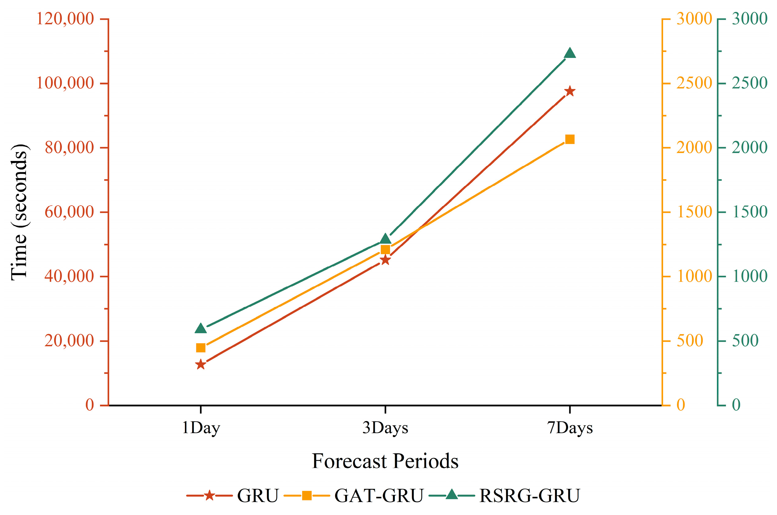
By comparing the training times of the three models, as shown in Figure 8, the GRU model required approximately 20 to 50 times longer to train across the 40 stations than the other two models. The training time of the GAT-GRU model for the 7-day forecast horizon was even less than 1/40 of that of the GRU model. This is because the GRU model must be trained separately for each station, whereas the GAT-GRU and ESRG-GRU models incorporate a Graph Attention Network (GAT) to capture spatial dependencies between stations, enabling parallel processing of data from all 40 stations within a single model, which significantly improves training efficiency. Compared to the GAT-GRU model, the ESRG-GRU model involves reconstructing the spatial adjacency matrix and introducing a novel hybrid loss function, resulting in increased training times of 31.567% (1-day), 6.230% (3-day), and 31.922% (7-day), respectively. Relative to the training time of the GRU model (taken as 1/40 of its actual duration), the ESRG-GRU model showed increases of 85.841% (1-day), 13.792% (3-day), and 11.837% (7-day). As the forecast horizon lengthens, the training efficiency of the ESRG-GRU model also progressively improves compared to that of the GRU model. These results demonstrate that the ESRG-GRU and GAT-GRU models, which incorporate graph structure and topological relationships, effectively utilize spatial correlations among stations, enable parallel computation across sites, and avoid the efficiency loss caused by repeated calculations in single-station models. Thus, they far outperform the GRU model in multi-station, long-term prediction efficiency, indicating that the spatiotemporally guided deep learning model incorporating graph structures holds considerable potential and value for practical applications involving long-term, synchronous multi-station forecasting.

3.3. Comparative Analysis of Model Accuracy

When comparing accuracy across different forecast horizons, our findings align with those of other studies: as the time step increases, the accuracy of the same model at the same station gradually decreases [38,50,51]. The decline in accuracy with longer forecast horizons can be attributed to two main factors. First, longer output sequences require the model to handle more extended and complex time-series data, where noise tends to accumulate more easily, thereby interfering with the model’s ability to understand intricate temporal relationships and leading to reduced prediction accuracy [52,53]. Second, as the input sequence length increases, the dependencies between the beginning and end of the sliding-window-processed data become weaker, making it harder for the model to capture correlations across distant time steps, which further exacerbates the decline in accuracy. To evaluate the improvement in model accuracy, we take the 7-day forecast horizon as an example for analysis.

3.3.1. Comparative Analysis of Model Accuracy: Spatial Pattern

In the 7-day forecasting period, as shown in Figure 9, the accuracy of the three models exhibits pronounced spatial heterogeneity across the study area. The 40 stations are divided into upper, middle, and lower reaches based on Shixincun and Yinshan Town as boundaries: stations above Shixincun are classified as upper reach, those at or below Yinshan Town as lower reach, and the remainder as middle reach.

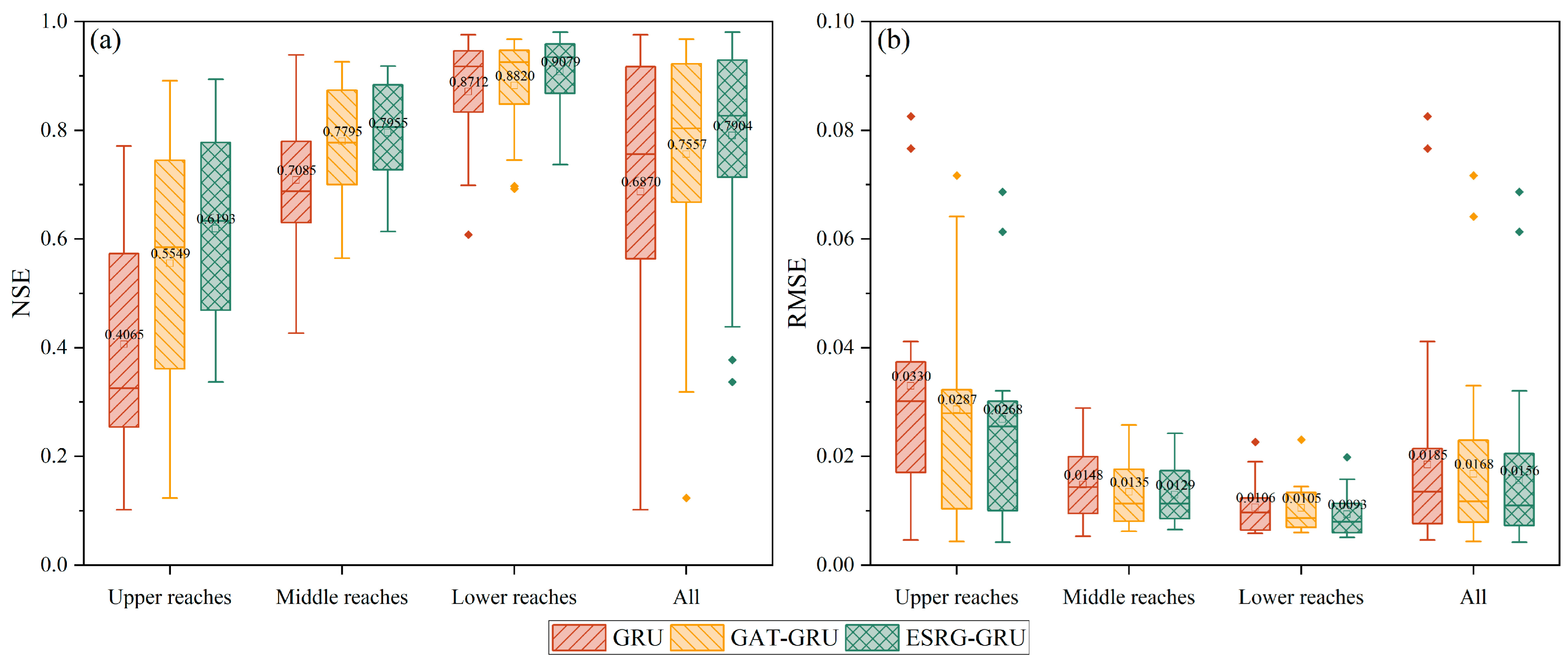
Across the entire basin, the average NSE values of the three models are 0.7904 (ESRG-GRU), 0.7557 (GAT-GRU), and 0.6870 (GRU), all falling within the “good” performance range. In the lower reach, the average NSE of all three models exceeds 0.8, with the ESRG-GRU model even surpassing 0.9. In contrast, in the upper reach, the average NSE of both the GAT-GRU and GRU models remains below 0.6, corresponding to “satisfactory” and “unsatisfactory” levels, respectively. The average RMSE values across the whole basin are all below 0.02—specifically, 0.0156 (ESRG-GRU), 0.0168 (GAT-GRU), and 0.0185 (GRU). However, in the upper reach, the average RMSE of all three models exceeds 0.02, with the GRU model reaching 0.033. These results indicate that incorporating physical spatiotemporal mechanisms effectively enhances the model’s ability to represent long-sequence data. Related studies also suggest that spatial information can improve a model’s capacity to learn complex patterns from data, as well as its generalization ability and prediction accuracy [54].

When comparing different regions using the same model, the average NSE consistently follows the order lower reach > middle reach > upper reach, while the average RMSE shows the opposite trend: lower reach < middle reach < upper reach. This indicates that, spatially, the models capture the dynamic variations in water quality more effectively in the lower reach than in the upper reach, leading to more accurate predictions downstream. The lower prediction accuracy for the upper reach may be attributed to the strongly nonlinear and abrupt characteristics of water quality parameters in that region. The more rugged mountainous terrain in the upper reach makes the area more susceptible to localized heavy rainfall and direct surface runoff, which increases input data uncertainty and makes it more challenging for models to capture underlying water quality patterns, thereby limiting predictive performance. In contrast, flow conditions are more stable in the middle and lower reaches, where water quality varies less abruptly, making it easier for models to learn and forecast.

When comparing the three models within the same region, the average NSE consistently ranks as ESRG-GRU > GAT-GRU > GRU, and the average RMSE as ESRG-GRU < GAT-GRU < GRU. This indicates that the ESRG-GRU model achieves the best overall prediction performance across stations in each region. In the 7-day long-term forecast, both the GAT-GRU and ESRG-GRU models demonstrate higher accuracy than the GRU model, likely because they incorporate graph-structural features, which provide an advantage in capturing long-term temporal dependencies [30]. The ESRG-GRU model, in particular, strengthens spatiotemporal dynamic modeling through physically meaningful graph structures. When handling long sequences, its built-in extremum-sensitive penalty and spatially weighted mechanisms help filter out noise interference to some extent, thereby maintaining more stable prediction accuracy.

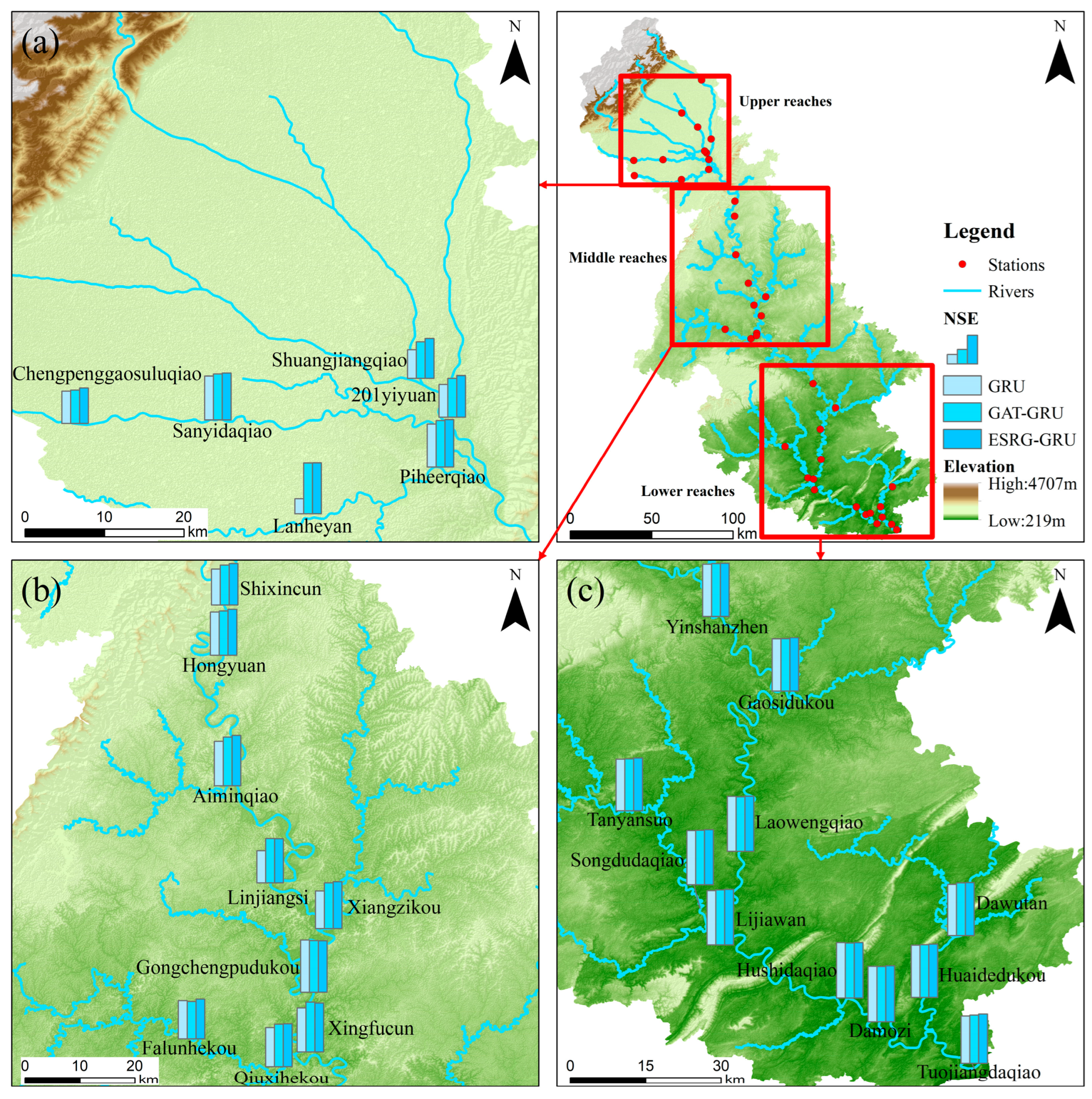
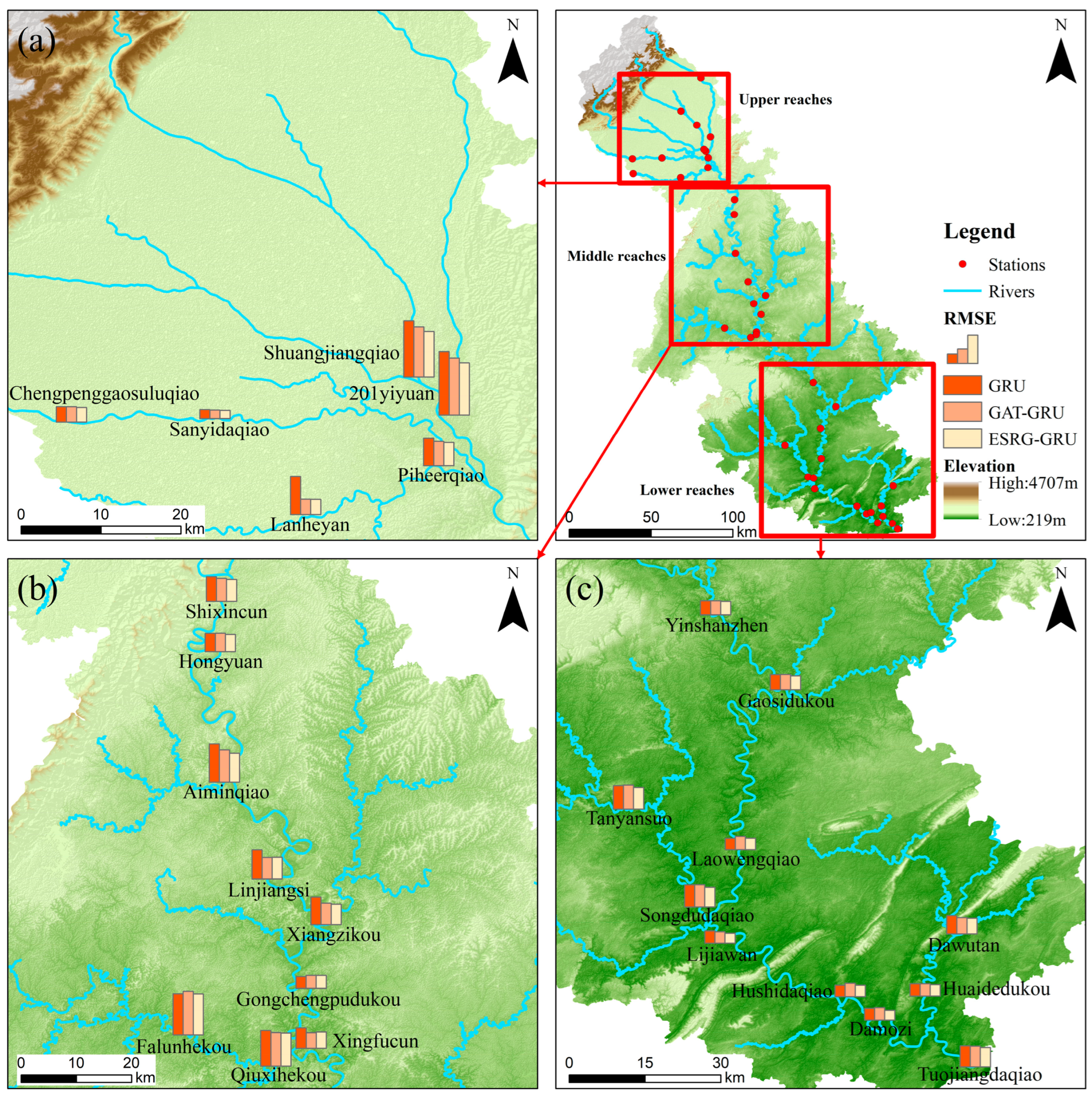
The distribution of NSE and RMSE values for selected representative stations is shown in Figure 10 and Figure 11. The accuracy performance of upstream stations is consistent with the regional patterns observed across the study area. The NSE values at upstream sites generally follow the order ESRG-GRU > GAT-GRU > GRU, and within the same tributary, higher NSE values are observed at downstream stations compared to upstream ones, while RMSE values show the opposite trend. Further upstream, the increasing proportion of mountainous terrain enhances river instability and susceptibility to extreme events, which intensifies nonlinear fluctuations in water quality [55,56], posing greater challenges for model learning and prediction.

The accuracy patterns at midstream representative stations are largely similar to those upstream. However, at some sites—such as Gongchengpudukou—the GRU model slightly outperforms the GAT-GRU and ESRG-GRU models. For instance, at this station, the GRU model achieves an NSE of 0.9165, while the GAT-GRU and ESRG-GRU models attain 0.9043 and 0.9031, respectively. The corresponding RMSE values are GRU (0.00609) < GAT-GRU (0.00674) < ESRG-GRU (0.00675). This may be attributed to the complex hydrological characteristics in certain midstream reaches, such as multiple tributary confluences and sediment-driven pollutant transport processes, which introduce strong local variability. Single-station trained models like the GRU can capture unique temporal variations at individual sites and thus perform well under such conditions. In contrast, graph-based models like GAT-GRU and ESRG-GRU, which learn from all stations simultaneously within the network, face greater challenges in capturing localized complex dynamics.

In downstream areas, the accuracy of the three models is generally similar, with only minor differences overall, though the ESRG-GRU model shows slightly better performance. The NSE values of the three models at representative downstream stations are very close, with ESRG-GRU being marginally higher. The RMSE of the ESRG-GRU model is generally lower than that of the other two models at most downstream sites, while the RMSE of the GAT-GRU model often exceeds that of the GRU model at more stations. This likely results from the gentle terrain and stable flow conditions in the lower reaches, where water quality varies more smoothly, making it easier for models to learn and predict, thus leading to less pronounced differences in model accuracy.

3.3.2. Comparative Analysis of Model Accuracy: Temporal Pattern

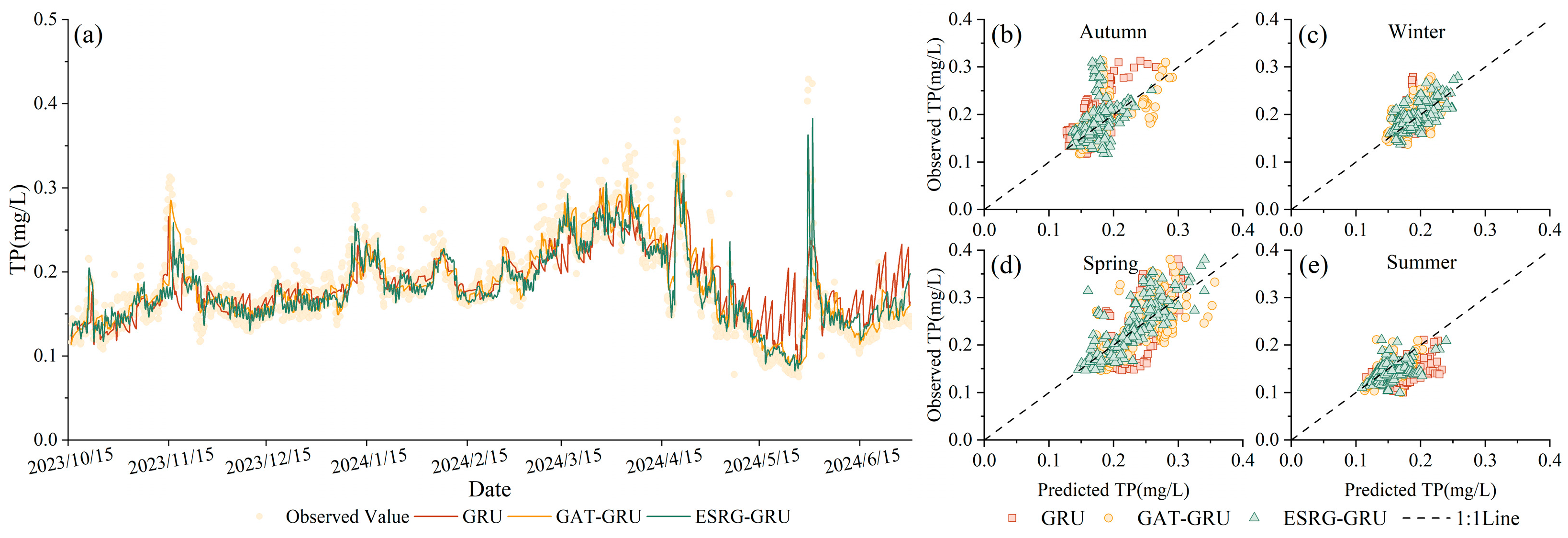
We selected November, January, April, and June as representative months for autumn, winter, spring, and summer, respectively, and analyzed the TP concentrations at one typical station from each reach: the upper reach (201yiyuan), the middle reach (Hongyuan), and the lower reach (Damozi).

As shown in Figure 12a, at the upper-reach 201 Hospital station, water quality fluctuated considerably during spring (March–May 2024), ranging approximately between 0.10 mg/L and 0.40 mg/L, while fluctuations were smaller in winter (December 2023–February 2024), with values mostly between 0.15 mg/L and 0.25 mg/L. Figure 12b–e reveal that the predicted values of the three models for typical months exhibit clear seasonal dependence. Overall, the ESRG-GRU predictions are more closely distributed around the 1:1 line, though underestimation occurs more frequently in spring and autumn, with some points showing larger deviations. In autumn, the GRU model tends to underestimate, whereas the GAT-GRU model more often overestimates. During winter, when water quality varies less, all three models produce predictions close to the observed values. In spring, the predictions are the most scattered among all seasons; the GRU and GAT-GRU models show more overestimation compared to the ESRG-GRU model. In summer, the GRU model predictions mostly lie below the 1:1 line, indicating a tendency to overestimate, with some overestimations being relatively large.

As presented in Figure 13a, at the middle-reach Hongyuan station, water quality varied widely in spring (March–May), ranging approximately from 0.05 mg/L to 0.20 mg/L, while fluctuations were smaller in autumn and winter (October 2023–February 2024), mostly between 0.05 mg/L and 0.10 mg/L. Figure 13b–e show that the distributions of the three models are generally similar. In autumn and winter, predictions from all three models cluster around the 1:1 line. In summer, most predictions from the GRU and ESRG-GRU models fall below the 1:1 line, indicating frequent overestimation, whereas the GAT-GRU model has a larger proportion of points above the line compared to the other two. During spring, predictions from all three models are more scattered, with many points deviating from the observed values, suggesting that the prediction of extremes requires further improvement.

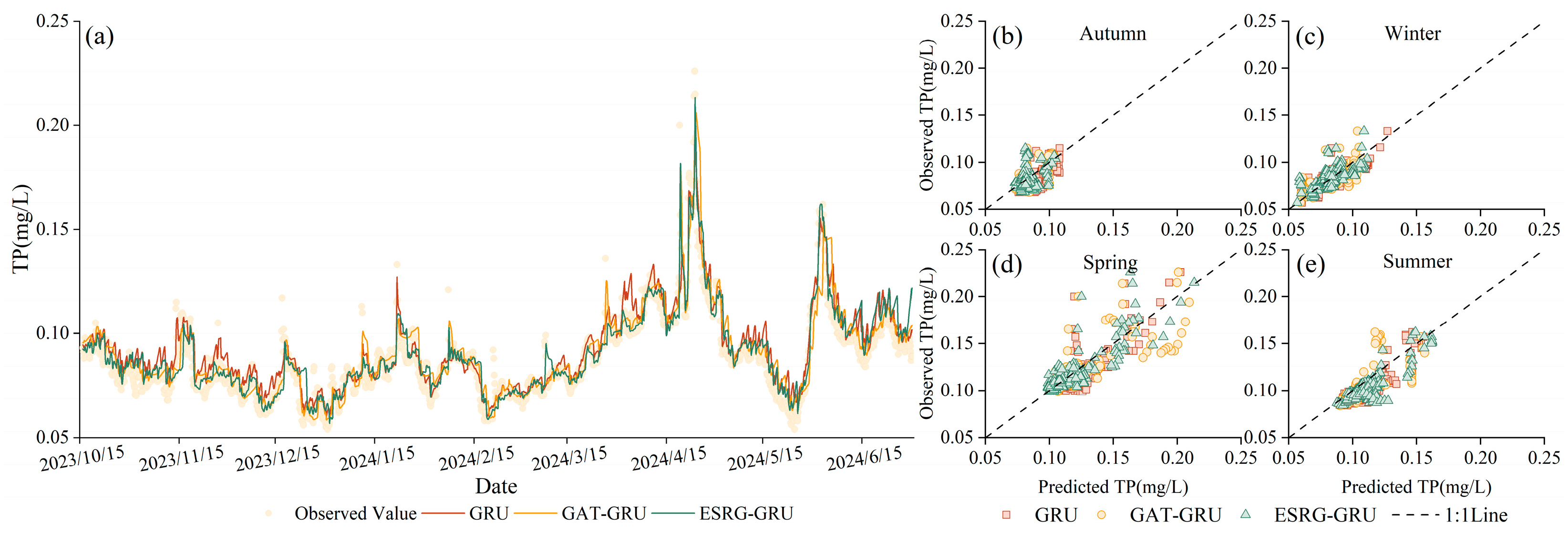
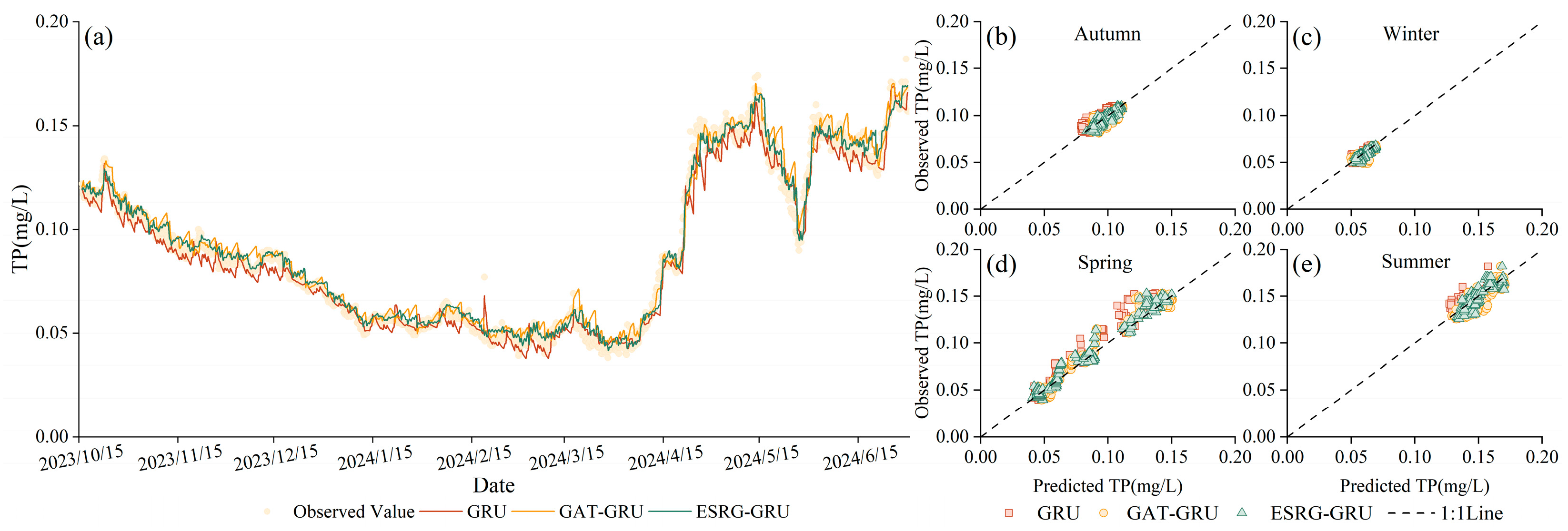
From both the time-series concentration comparison in Figure 14a and the scatter distributions relative to the 1:1 line in Figure 14b–e, it can be seen that the GRU predictions often lie below the observed values. Except in winter, where the underestimation is less pronounced, the GRU model shows noticeably lower predictions than the other two models in spring, summer, and autumn. Predictions from all three models cluster closely around the 1:1 line in autumn and winter, whereas they are more dispersed in spring and summer. The spring representative month (April) reveals large variations in TP concentration at Damozi; as seen in Figure 14a, the concentration rose from below 0.05 mg/L to about 0.15 mg/L—a threefold increase within a month. In the summer representative month (June), the GAT-GRU model has more points below the 1:1 line, indicating that it overestimates more frequently than the other two models. In contrast, the ESRG-GRU model predictions are more tightly distributed along the 1:1 line and show the smallest deviation from the observed values.

In the study area, TP concentrations exhibited smaller variations in winter compared to other seasons, while showing significant fluctuations in spring, indicating clear seasonal variability. This seasonality is reflected in model accuracy: all three models produced predictions closer to observed values in winter, whereas in spring, instances of overestimation and underestimation increased markedly. Some predicted values from the GRU, GAT-GRU, and ESRG-GRU models displayed similar or even overlapping trends. This phenomenon suggests that, despite differences in model architecture, under extreme conditions, the predictive performance of all models may be jointly constrained by sparse data distribution and nonlinear dynamics, resulting in a weaker ability to capture abrupt changes.

The dispersion of predictions increased significantly in spring. On one hand, this can be attributed to the aggravated error accumulation effect in long-sequence forecasting [52]. On the other hand, increased rainfall in late spring and early summer triggers nonlinear hydrological processes [56]. Coupled with seasonal pollutant discharges and transport from human activities, these factors lead to higher TP concentrations and greater variability in spring and summer, resulting in pronounced lag and nonlinearity in water quality responses. The GRU model, lacking the ability to model spatial correlations, struggles to accurately capture the transport and diffusion of pollutants across the basin, leading to larger prediction deviations. Although the ESRG-GRU and GAT-GRU models partially capture these nonlinear relationships through spatiotemporal graph structures, and also show increased dispersion in spring predictions, their results remain closer to the 1:1 line compared to the GRU model. This indicates that while these models do not fully represent the underlying dynamic mechanisms, the physically informed constraints still enhance model stability in long-sequence forecasting [28].

3.3.3. Analysis of Model Accuracy Improvement

Compared to the GAT-GRU model, the ESRG-GRU model achieved an overall improvement in NSE of 11.64% in the upper reach, 2.05% in the middle reach, and 2.94% in the lower reach. Although the accuracy gain was most pronounced in the upper reach, the mean NSE of the ESRG-GRU model there remained relatively low at 0.6193, compared to 0.7955 in the middle reach and 0.9079 in the lower reach, indicating that model performance was still comparatively poor in upstream areas.

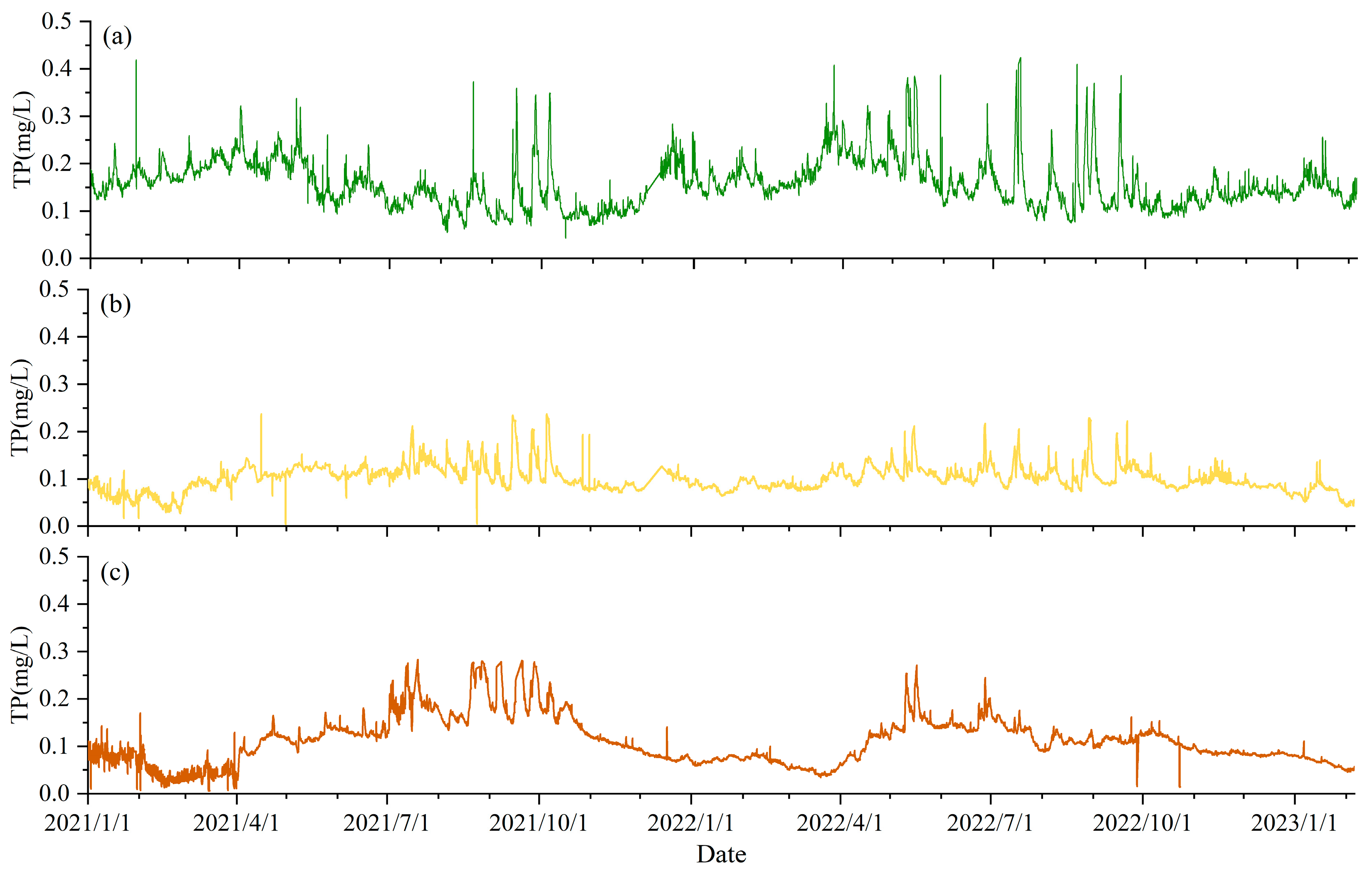
Model accuracy is influenced by data quality, feature selection, and model architecture. In terms of data quality, the upper reach data were generally inferior to those from the middle and lower reaches. Taking the TP training data from typical stations in each reach as an example (Figure 15), the TP concentration at the upstream station 201yiyuan exhibited much more pronounced fluctuations than at the middle-reach station Hongyuan and the downstream station Damozi. Moreover, Figure 15a for 201yiyuan shows a considerable number of high-value outliers that contrast sharply with surrounding data points. This is likely due to the station’s upstream location, where water quality is more susceptible to localized, episodic events such as heavy rainfall or sporadic pollutant discharges, and may also reflect irregular operation of the automatic monitoring or sampling equipment. In contrast, the downstream station Damozi displayed only a few obvious low- and high-value outliers, with generally stable water quality, indicating clearly superior data quality. Additionally, the meteorological data used during training were derived from daily values interpolated to hourly resolution via nearest-neighbor interpolation. Hydrological responses are faster in upstream areas, and the original temporal resolution of the data may be insufficient to fully capture such rapid dynamics.

Regarding feature selection, limited data availability restricted the inclusion of other key spatial processes—such as land use and point-source pollution locations—and dynamic temporal drivers—such as real-time dam operations, flow rate, velocity, and point-source discharge processes. As a result, deeper embedding of physical process mechanisms into the model remains an area for further improvement.

Architecturally, for the two graph-neural-network-based models—especially the ESRG-GRU model—learning depends on information aggregated from upstream stations. Some stations, however, have few or no upstream stations, meaning that during message passing, they receive little or no information from other water quality sites and must rely primarily on their own limited historical temporal features. This effectively reduces a complex spatiotemporal forecasting problem to an almost purely temporal prediction task, preventing the model from leveraging spatial correlations to correct errors or learn cross-station propagation patterns.

In response to these challenges, we aim to integrate this data-driven framework with land use change data and real-time information on engineering operations, pollutant discharges, and hydrological monitoring. Through architectural design or loss-function constraints, we intend to further develop it into a truly “process-aware” model that more closely couples physical processes with deep learning. This approach is expected to enhance the model’s generalization ability and interpretability under non-stationary conditions [7], thereby better addressing water-environment management challenges posed by sudden pollution incidents and changing climate patterns. In the future, we will also validate the feasibility of the proposed method by applying it to multi-parameter joint forecasting in other river basins.

4. Conclusions

This study constructed three deep learning models—GRU, GAT-GRU, and ESRG-GRU—to predict water quality in the Tuojiang River Basin, Sichuan Province, China. We recorded the training duration of each model for forecast horizons of 1, 3, and 7 days. The ESRG-GRU and GAT-GRU models, which incorporate graph structure and topological relationships, required significantly less training time than the baseline GRU model, and their efficiency advantage became more pronounced as the forecast horizon increased. Compared to the GAT-GRU model, the ESRG-GRU model reconstructs the adjacency matrix and improves the loss function, leading to increased model complexity. However, its training time did not increase substantially and remains acceptable in practice. Using the NSE and RMSE values for the 7-day horizon to evaluate model accuracy, the ESRG-GRU model achieved a higher average NSE during the testing period compared to the other two models, with improvements of 0.1034 and 0.0347 over the GRU and GAT-GRU models, respectively. Its average RMSE decreased by 15.676% and 7.143% compared to the GRU and GAT-GRU models, demonstrating good predictive performance. Model accuracy showed clear spatiotemporal heterogeneity. Spatially, all three models performed best in the lower reach, followed by the middle reach, and least accurately in the upper reach. Temporally, predictions were closer to observations in winter, while the opposite was true in spring. These results demonstrate the feasibility of the enhanced spatiotemporal relationship-guided deep learning method proposed in this study for water quality prediction. This approach can improve both the training efficiency and prediction accuracy of long-term forecasting models, providing a valuable reference for multi-station water quality prediction over extended periods.

Limited by data availability, other key spatial processes—such as land use and point-source pollution locations—and dynamic temporal drivers—such as real-time dam operations, flow rate, velocity, and point-source discharge processes—were not included as input features. Moreover, the temporal resolution of the acquired meteorological data is relatively low, and data from some upstream stations exhibit considerable fluctuations, which, together, contribute to the lower prediction accuracy at upstream sites compared to middle and downstream stations. In the future, incorporating these additional data sources as model inputs and further integrating physical processes with deep learning are expected to enhance the model’s generalizability and interpretability under non-stationary conditions. Since graph-based models inherently offer a clear training-time advantage over separate per-station models, future work will also explore algorithmic innovations to further improve training efficiency. Additionally, the feasibility of the proposed method will be validated through multi-parameter joint forecasting in other river basins.

References

1. Giri, S. Water Quality Prospective in Twenty First Century: Status of Water Quality in Major River Basins, Contemporary Strategies and Impediments: A Review. Environ. Pollut. 2021, 271, 116332. [Google Scholar] [CrossRef] [PubMed]
2. van Vliet, M.; Jones, E.; Flörke, M.; Franssen, W.; Hanasaki, N.; Wada, Y.; Yearsley, J. Global Water Scarcity Including Surface Water Quality and Expansions of Clean Water Technologies. Environ. Res. Lett. 2021, 16, 024020. [Google Scholar] [CrossRef]
3. Wang, M.; Bodirsky, B.L.; Rijneveld, R.; Beier, F.; Bak, M.P.; Batool, M.; Droppers, B.; Popp, A.; van Vliet, M.T.H.; Strokal, M. A Triple Increase in Global River Basins with Water Scarcity Due to Future Pollution. Nat. Commun. 2024, 15, 880. [Google Scholar] [CrossRef]
4. Ma, T.; Sun, S.; Fu, G.; Hall, J.; Ni, Y.; He, L.; Yi, J.; Zhao, N.; Du, Y.; Pei, T.; et al. Pollution Exacerbates China’s Water Scarcity and Its Regional Inequality. Nat. Commun. 2020, 11, 650. [Google Scholar] [CrossRef]
5. LeCun, Y.; Bengio, Y.; Hinton, G. Deep Learning. Nature 2015, 521, 436–444. [Google Scholar] [CrossRef]
6. Zheng, Y.; Zhang, Q.; Zhang, X.; Zhou, Y.; Zhang, Y.; Zhang, T. A Spatial-Temporal Trend-Aware Neural Network Model for Accurate Water Quality Prediction in River. Water Res. 2025, 287, 124389. [Google Scholar] [CrossRef] [PubMed]
7. Zhi, W.; Appling, A.P.; Golden, H.E.; Podgorski, J.; Li, L. Deep Learning for Water Quality. Nat. Water 2024, 2, 228–241. [Google Scholar] [CrossRef]
8. Haghiabi, A.H.; Nasrolahi, A.H.; Parsaie, A. Water Quality Prediction Using Machine Learning Methods. Water Qual. Res. J. 2018, 53, 3–13. [Google Scholar] [CrossRef]
9. Yang, S.; Zhong, S.; Chen, K. W-WaveNet: A Multi-Site Water Quality Prediction Model Incorporating Adaptive Graph Convolution and CNN-LSTM. PLoS ONE 2024, 19, e0276155. [Google Scholar] [CrossRef]
10. Fang, P.; Wang, Y.; Zhao, Y.; Kang, J. Analysis of Prediction Confidence in Water Quality Forecasting Employing LSTM. Water 2025, 17, 1050. [Google Scholar] [CrossRef]
11. Li, L.; Jiang, P.; Xu, H.; Lin, G.; Guo, D.; Wu, H. Water Quality Prediction Based on Recurrent Neural Network and Improved Evidence Theory: A Case Study of Qiantang River, China. Environ. Sci. Pollut. Res. 2019, 26, 19879–19896. [Google Scholar] [CrossRef]
12. Wang, D.; Zhang, C.; Li, A.; Guo, Y.; Zhang, H.; Tan, C. Spatio-Temporal Analysis and Prediction for Raw Water Quality of Drinking Water Source by Improved RNN Algorithm. J. Water Process Eng. 2025, 71, 107164. [Google Scholar] [CrossRef]
13. Li, Q.; Yang, Y.; Yang, L.; Wang, Y. Comparative Analysis of Water Quality Prediction Performance Based on LSTM in the Haihe River Basin, China. Environ. Sci. Pollut. Res. 2023, 30, 7498–7509. [Google Scholar] [CrossRef] [PubMed]
14. Pyo, J.; Pachepsky, Y.; Kim, S.; Abbas, A.; Kim, M.; Kwon, Y.S.; Ligaray, M.; Cho, K.H. Long Short-Term Memory Models of Water Quality in Inland Water Environments. Water Res. X 2023, 21, 100207. [Google Scholar] [CrossRef]
15. Luo, L.; Zhang, Y.; Dong, W.; Zhang, J.; Zhang, L. Ensemble Empirical Mode Decomposition and a Long Short-Term Memory Neural Network for Surface Water Quality Prediction of the Xiaofu River, China. Water 2023, 15, 1625. [Google Scholar] [CrossRef]
16. Lee, J.; Lee, J.; Lee, M.; Lee, M.; Kim, Y.; Hyung, J.; Kim, K.; Cha, Y.; Koo, J. Development of a Short-Term Water Quality Prediction Model for Urban Rivers Using Real-Time Water Quality Data. Water Supply 2022, 22, 4082–4097. [Google Scholar] [CrossRef]
17. Li, W.; Wu, H.; Zhu, N.; Jiang, Y.; Tan, J.; Guo, Y. Prediction of Dissolved Oxygen in a Fishery Pond Based on Gated Recurrent Unit (GRU). Inf. Process. Agric. 2021, 8, 185–193. [Google Scholar] [CrossRef]
18. Yang, H.; Liu, S. Water Quality Prediction in Sea Cucumber Farming Based on a GRU Neural Network Optimized by an Improved Whale Optimization Algorithm. Peer J. Comput. Sci. 2022, 8, e1000. [Google Scholar] [CrossRef]
19. Xu, J.; Wang, K.; Lin, C.; Xiao, L.; Huang, X.; Zhang, Y. FM-GRU: A Time Series Prediction Method for Water Quality Based on Seq2seq Framework. Water 2021, 13, 1031. [Google Scholar] [CrossRef]
20. Zhang, Y.; Liu, L.; Zhang, S.; Zou, X.; Liu, J.; Guo, J.; Teng, Y.; Zhang, Y.; Duan, H. Monitoring and Warning for Ammonia Nitrogen Pollution of Urban River Based on Neural Network Algorithms. Anal. Sci. 2024, 40, 1867–1879. [Google Scholar] [CrossRef]
21. Zhendong, Z.; Hui, Q.; Liqiang, Y.; Yongqi, L.; Zhiqiang, J.; Zhongkai, F.; Shuo, O.; Shaoqian, P.; Jianzhong, Z. Downstream Water Level Prediction of Reservoir Based on Convolutional Neural Network and Long Short-Term Memory Network. J. Water Resour. Plan. Manag. 2021, 147, 04021060. [Google Scholar] [CrossRef]
22. Tian, Q.; Luo, W.; Guo, L. Water Quality Prediction in the Yellow River Source Area Based on the DeepTCN-GRU Model. J. Water Process Eng. 2024, 59, 105052. [Google Scholar] [CrossRef]
23. Haq, K.; Harigovindan, V. Water Quality Prediction for Smart Aquaculture Using Hybrid Deep Learning Models. IEEE Access 2022, 10, 60078–60098. [Google Scholar] [CrossRef]
24. Mei, P.; Li, M.; Zhang, Q.; Li, G.; Song, L. Prediction Model of Drinking Water Source Quality with Potential Industrial-Agricultural Pollution Based on CNN-GRU-Attention. J. Hydrol. 2022, 610, 127934. [Google Scholar] [CrossRef]
25. Chen, H.; Yang, J.; Fu, X.; Zheng, Q.; Song, X.; Fu, Z.; Wang, J.; Liang, Y.; Yin, H.; Liu, Z.; et al. Water Quality Prediction Based on LSTM and Attention Mechanism: A Case Study of the Burnett River, Australia. Sustainability 2022, 14, 13231. [Google Scholar] [CrossRef]
26. Yang, Y.; Xiong, Q.; Wu, C.; Zou, Q.; Yu, Y.; Yi, H.; Gao, M. A Study on Water Quality Prediction by a Hybrid CNN-LSTM Model with Attention Mechanism. Environ. Sci. Pollut. Res. 2021, 28, 55129–55139. [Google Scholar] [CrossRef]
27. Bi, J.; Chen, Z.; Yuan, H.; Zhang, J. Accurate Water Quality Prediction with Attention-Based Bidirectional LSTM and Encoder-Decoder. Expert Syst. Appl. 2024, 238, 121807. [Google Scholar] [CrossRef]
28. Qiao, J.; Lin, Y.; Bi, J.; Yuan, H.; Wang, G.; Zhou, M. Attention-Based Spatiotemporal Graph Fusion Convolution Networks for Water Quality Prediction. IEEE Trans. Autom. Sci. Eng. 2025, 22, 1–10. [Google Scholar] [CrossRef]
29. Nie, Q.; Wan, D.; Wang, R. CNN-BiLSTM Water Level Prediction Method with Attention Mechanism. J. Phys. Conf. Ser. 2021, 2078, 012032. [Google Scholar] [CrossRef]
30. Wan, H.; Xiang, L.; Cai, Y.; Xie, Y.; Xu, R. Temporal and Spatial Feature Extraction Using Graph Neural Networks for Multi-Point Water Quality Prediction in River Network Areas. Water Res. 2025, 281, 123561. [Google Scholar] [CrossRef]
31. Li, Z.; Liu, H.; Zhang, C.; Fu, G. Real-Time Water Quality Prediction in Water Distribution Networks Using Graph Neural Networks with Sparse Monitoring Data. Water Res. 2024, 250, 121018. [Google Scholar] [CrossRef]
32. Sheng, Z.; Cai, Z. GAT-GRU Based Model for Water Network Flow Prediction. In Proceedings of the 9th International Conference on Water Resource and Environment; Weng, C.-H., Ed.; Springer Nature: Singapore, 2024; pp. 151–162. [Google Scholar]
33. Song, J.; Meng, H.; Kang, Y.; Zhu, M.; Zhu, Y.; Zhang, J. A Method for Predicting Water Quality of River Basin Based on OVMD-GAT-GRU. Stoch. Environ. Res. Risk Assess. 2024, 38, 339–356. [Google Scholar] [CrossRef]
34. Sun, C.; Li, C.; Lin, X.; Zheng, T.; Meng, F.; Rui, X.; Wang, Z. Attention-Based Graph Neural Networks: A Survey. Artif. Intell. Rev. 2023, 56, 2263–2310. [Google Scholar] [CrossRef]
35. Chen, S.; Gan, Z.; Li, Z.; Li, Y.; Ma, X.; Chen, M.; Qu, B.; Ding, S.; Su, S. Occurrence and Risk Assessment of Anthelmintics in Tuojiang River in Sichuan, China. Ecotoxicol. Environ. Saf. 2021, 220, 112360. [Google Scholar] [CrossRef]
36. Xu, J.; Wang, Y.; Chen, Y.; Tong, H.; Wei, Y.; Bai, H. Characteristics on Spatiotemporal Variations of Surface Water Environmental Quality in Tuojiang River in Upper Reaches of Yangtze River Basin. Earth Sci. 2019, 45, 1937. [Google Scholar] [CrossRef]
37. Wei, X.; Zhang, L.; Yang, H.-Q.; Zhang, L.; Yao, Y.-P. Machine Learning for Pore-Water Pressure Time-Series Prediction: Application of Recurrent Neural Networks. Geosci. Front. 2021, 12, 453–467. [Google Scholar] [CrossRef]
38. Zuo, Y.; Jiang, J.; Yada, K. Application of Hybrid Gate Recurrent Unit for In-Store Trajectory Prediction Based on Indoor Location System. Sci. Rep. 2025, 15, 1055. [Google Scholar] [CrossRef] [PubMed]
39. Rahul Gandh, D.; Harigovindan, V.P.; Rasheed Abdul Haq, K.P.; Bhide, A. Attention-Driven LSTM and GRU Deep Learning Techniques for Precise Water Quality Prediction in Smart Aquaculture. Aquacult. Int. 2024, 32, 8455–8478. [Google Scholar] [CrossRef]
40. Corradini, F.; Gerosa, F.; Gori, M.; Lucheroni, C.; Piangerelli, M.; Zannotti, M. A Systematic Literature Review of Spatio-Temporal Graph Neural Network Models for Time Series Forecasting and Classification. Neural Netw. 2026, 195, 108269. [Google Scholar] [CrossRef]
41. Chen, R.; Lin, K.; Hong, B.; Zhang, S.; Yang, F. Sparse Graphs-Based Dynamic Attention Networks. Heliyon 2024, 10, e35938. [Google Scholar] [CrossRef]
42. Wu, Z.; Pan, S.; Chen, F.; Long, G.; Zhang, C.; Yu, P. A Comprehensive Survey on Graph Neural Networks. IEEE Trans. Neural Netw. Learn. Syst. 2021, 32, 4–24. [Google Scholar] [CrossRef]
43. Veličković, P.; Cucurull, G.; Casanova, A.; Romero, A.; Lio, P.; Bengio, Y. Graph Attention Networks. arXiv 2017, arXiv:1710.10903. [Google Scholar] [CrossRef]
44. Jenson, S.; Domingue, J. Extracting Topographic Structure from Digital Elevation Data for Geographic Information-System Analysis. Photogramm. Eng. Remote Sens. 1988, 54, 1593–1600. [Google Scholar]
45. Xu, W.; Chen, K.; Han, T.; Chen, H.; Ouyang, W.; Bai, L. Extremecast: Boosting Extreme Value Prediction for Global Weather Forecast. arXiv 2024, arXiv:2402.01295. [Google Scholar] [CrossRef]
46. Richard, H.M.; Zachary, K.; Cutter, A.G. Evaluation of the Nash–Sutcliffe Efficiency Index. J. Hydrol. Eng. 2006, 11, 597–602. [Google Scholar] [CrossRef]
47. Hodson, T.O. Root-Mean-Square Error (RMSE) or Mean Absolute Error (MAE): When to Use Them or Not. Geosci. Model Dev. 2022, 15, 5481–5487. [Google Scholar] [CrossRef]
48. Moriasi, D.N.; Gitau, M.W.; Pai, N.; Daggupati, P. Hydrologic and Water Quality Models: Performance Measures and Evaluation Criteria. Trans. ASABE 2015, 58, 1763–1785. [Google Scholar] [CrossRef]
49. Khan, A.; Cao, X.; Li, S.; Katsikis, V.; Liao, L. BAS-ADAM: An ADAM Based Approach to Improve the Performance of Beetle Antennae Search Optimizer. IEEE/CAA J. Autom. Sin. 2020, 7, 461–471. [Google Scholar] [CrossRef]
50. Xie, L.; Zhao, Y.; Fang, P.; Cheng, M.; Chen, Z.; Wang, Y. A Novel Operational Water Quality Mobile Prediction System with LSTM-Seq2Seq Model. Environ. Model. Softw. 2025, 185, 106290. [Google Scholar] [CrossRef]
51. Sabzipour, B.; Arsenault, R.; Troin, M.; Martel, J.-L.; Brissette, F.; Brunet, F.; Mai, J. Comparing a Long Short-Term Memory (LSTM) Neural Network with a Physically-Based Hydrological Model for Streamflow Forecasting over a Canadian Catchment. J. Hydrol. 2023, 627, 130380. [Google Scholar] [CrossRef]
52. Liu, Y.; Wang, Y. Water Quality Prediction Method Based on a Combined Machine Learning Model: A Case Study of the Daling River Basin. J. Contam. Hydrol. 2026, 276, 104725. [Google Scholar] [CrossRef] [PubMed]
53. Wang, Z.; Sun, Z.; Bian, Y.; Mo, H.; Dong, D. Learning Hierarchical Time–Frequency Representation for Long-Term Time Series Forecasting. Inf. Process. Manag. 2026, 63, 104358. [Google Scholar] [CrossRef]
54. Lei, Y.; Hu, B.; Huang, H.; Liu, Y. Design of a Variable-Length Sequential Prediction Framework GTV-STP Based on Spatial and Temporal Water Quality Information of Taihu Lake. IEEE Access 2024, 12, 65928–65941. [Google Scholar] [CrossRef]
55. Kirchner, J. Characterizing Nonlinear, Nonstationary, and Heterogeneous Hydrologic Behavior Using Ensemble Rainfall-Runoff Analysis (ERRA): Proof of Concept. Hydrol. Earth Syst. Sci. 2024, 28, 4427–4454. [Google Scholar] [CrossRef]
56. Liu, L.; Ye, S.; Chen, C.; Pan, H.; Ran, Q. Nonsequential Response in Mountainous Areas of Southwest China. Front. Earth Sci. 2021, 9, 660244. [Google Scholar] [CrossRef]
Figure 1. Overview of the study area.
Water 18 00185 g001
Figure 2. Internal structure diagram of the GRU.
Water 18 00185 g002
Figure 3. Framework diagram of the GRU model.
Water 18 00185 g003
Figure 4. AT attention mechanism.
Water 18 00185 g004
Figure 5. Structure of the GAT-GRU model.
Water 18 00185 g005
Figure 6. Generalized topological relationship of river network.
Water 18 00185 g006
Figure 7. ESRG-GRU training process.
Water 18 00185 g007
Figure 8. Training durations of models with different forecast periods.
Water 18 00185 g008
Figure 9. Comparison of the accuracy of different models in different regions: (a) NSE of different models in different regions; (b) RMSE of different models in different regions.
Water 18 00185 g009
Figure 10. Comparison of NSE values at typical sites of different models: (a) NSE values of different models for typical upstream regional sites; (b) NSE values of different models for typical midstream regional sites; (c) NSE values of different models for typical downstream regional sites.
Water 18 00185 g010
Figure 11. Comparison of RMSE values at typical sites of different models: (a) RMSE values of different models for typical upstream regional sites; (b) RMSE values of different models for typical midstream regional sites; (c) RMSE values of different models for typical downstream regional sites.
Water 18 00185 g011
Figure 12. Comparison of observed and measured TP concentration values during the 201yiyuan test: (a) Predicted values and observed values of the three models during the test period. (b) Predicted values and observed values of the three models in typical autumn months. (c) Predicted values and observed values of the three models in typical winter months. (d) Predicted values and observed values of the three models in typical spring months. (e) Predicted values and observed values of the three models in typical summer months.
Water 18 00185 g012
Figure 13. Comparison of observed and measured TP concentration values during the Hongyuan test: (a) Predicted values and observed values of the three models during the test period. (b) Predicted values and observed values of the three models in typical autumn months. (c) Predicted values and observed values of the three models in typical winter months. (d) Predicted values and observed values of the three models in typical spring months. (e) Predicted values and observed values of the three models in typical summer months.
Water 18 00185 g013
Figure 14. Comparison of observed and measured TP concentration values during the Damozi test: (a) Predicted values and observed values of the three models during the test period. (b) Predicted values and observed values of the three models in typical autumn months. (c) Predicted values and observed values of the three models in typical winter months. (d) Predicted values and observed values of the three models in typical spring months. (e) Predicted values and observed values of the three models in typical summer months.
Water 18 00185 g014
Figure 15. Comparison of model training data from representative stations in different river reaches: (a) 201 Hospital station in the upper reach. (b) Hongyuan station in the middle reach. (c) Damozi station in the lower reach.
Water 18 00185 g015
Disclaimer/Publisher’s Note: The statements, opinions and data contained in all publications are solely those of the individual author(s) and contributor(s) and not of MDPI and/or the editor(s). MDPI and/or the editor(s) disclaim responsibility for any injury to people or property resulting from any ideas, methods, instructions or products referred to in the content.