Assessing Rating Curves in River Gauging Stations for Computing Design Extreme Events for Several Return Periods

Abstract

Rating curves are derived from the combined measurement of water levels and discharges in rivers. This curve is used to convert observed water levels into flow rates, thereby generating discharge time series. Traditionally, rating curves are computed using exponential regression, which often neglects the underlying hydraulic conditions. Consequently, such curves may provide reasonable estimates of average flow but become unreliable under extreme conditions (e.g., high water levels). This research proposes a strategy for estimating discharge at high water levels using hydraulic modelling to support designers and practitioners in interpreting the upper range of the stage–discharge relationship. The methodology was applied to assess the rating curve for high flows in the Magdalena River at the Magangué reach (Bolívar, Colombia). Daily discharge records from 1974 to 2023 were analysed. The maximum historical discharge recorded was 11,127 m³/s (in 2010), while the mean annual peak discharge was 7904 m³/s. The proposed methodology yielded Manning’s roughness coefficients ranging from 0.046 to 0.052 and achieved satisfactory performance, with a Nash–Sutcliffe Efficiency (NSE) of 0.99. Results demonstrated that the traditional regression-based method tends to underestimate maximum discharges relative to a properly calibrated upper section of the rating curve. The analysis revealed systematic underestimation by the conventional approach, with discrepancies of up to 4.2% in determining maximum discharges. These findings emphasise the importance of incorporating hydraulic modelling to refine rating curves for high-flow conditions, thereby improving the reliability of design discharges.

1. Introduction

Discharge measurements are of utmost importance for an adequate characterisation of rivers. In this context, hydrological agencies worldwide commonly install river gauging stations to support the planning of major infrastructure projects, such as hydropower developments. These stations require a velocity sample at several vertical levels within a cross-sectional area to compute water flow and the corresponding water level. It implies that water flow is indirectly measured. This procedure is known as the stage-discharge rating curve [1].

Rating curves are typically derived using exponential regression, expressed as $Q=a(WL-W{L}_0{)}^b$, where $Q$ represents the discharge, $WL$ is the corresponding water level, $W{L}_0$ denotes the reference level, and $a$ and $b$ are the regression constants [2].

Ali and Maghrebi (2023) [3] computed rating curves under data-scarce conditions and analysed the associated uncertainty. More recently, machine learning techniques have been employed to evaluate the behaviour of rating curves using various algorithms, such as support vector machines and neural networks [4,5,6].

Discharge and water-level calibration can be assessed using hydraulic approaches. In this sense, hydraulic modeling is a fundamental tool for understanding and managing fluvial processes, especially in regions where extreme events, such as floods, pose a constant risk to riparian communities [7]. In this context, accurate model calibration is essential to ensure that simulations faithfully reproduce the hydraulic system’s actual behavior [8]. One of the most widely used programs worldwide for this purpose is HEC-RAS, developed by the U.S. Army Corps of Engineers, which simulates flows in natural or artificial channels under different flow conditions [9]. Several studies have demonstrated the usefulness of HEC-RAS for flood analysis and model calibration in rivers of various scales. For example, the study by [10] analyzed uncertainty in roughness parameter calibration in HEC-RAS using the GLUE method. Their results showed that multiple combinations of roughness values can reproduce both flood extent and outflow hydrographs with similar accuracy, thereby highlighting the concept of equifinality. In Latin America, Bruno et al. [11] applied a coupled hydrological–hydraulic model (HEC-HMS and HEC-RAS) to a small urban basin in Brazil, using high-resolution data. The results showed a good fit in calibration and validation (R² = 0.93 and NSE = 0.92). They simulated flood scenarios for return periods of 5, 10, 50, and 100 years, concluding that this approach improves the representation of local dynamics and supports the planning of adaptation measures against urban flooding. In Colombia, Santos et al. [12] applied a one-dimensional HEC-RAS model to simulate the hydraulic behavior of the Magdalena River in the Calamar area, where the diversion toward the Canal del Dique occurs. Using bathymetric surveys and hydrometric records, the authors calibrated and validated the model, obtaining a satisfactory fit between observed and simulated discharges (Nash–Sutcliffe = 0.98), demonstrating that HEC-RAS can accurately represent discharge distribution in large rivers with diversions. However, they highlighted the limitations of manual multi-objective calibration. On the other hand [13], applied a river model calibration method based on Design of Experiments (DOE) theory, evaluating a 75 km reach of the Meta River using the MIKE-21C model and obtaining an overall performance index of 0.857, concluding that this systematic method improves the reliability of hydromorphological models by accounting for parameter interactions and can be applied to both 1D and 2D models.

Current studies on rating curves are mainly focused on developing computational applications (e.g., in Python) [14], assessing the uncertainty in their estimation [15,16], analysing rating curves derived from limited datasets [17], and making predictions using machine-learning methods [18].

One of the main limitations in current studies is the determination of rating curves at high water levels, which are essential for estimating extreme discharges that are not typically captured by hydrological measurements. In this regard, this portion of the curve can only be estimated through appropriate calibration using a model that accounts for the river reach’s geometric characteristics.

This research proposes a methodology for computing rating curves at high water levels in rivers based on geometric characteristics and hydraulic modelling. The resulting framework consolidates best-practice guidelines that engineers and designers can apply to reliably estimate extreme events. This methodology is crucial to ensure that the determination of maximum water flows is accurately interpreted and used to compute extreme flows for different return periods. In this research, the Magdalena River reach in the Magangué Municipality, Colombia, was selected as a case study. In Colombia, the Magdalena River is the country’s most crucial fluvial artery, both economically and environmentally [19]. Its lower basin, particularly the reach that crosses the municipality of Magangué (Bolívar), is characterized by flat topography, high sedimentation rates, and intense vulnerability to flooding [20]. This area, located in the Momposina Depression, is subject to recurrent flooding, which causes severe socioeconomic impacts. These factors necessitate the development of reliable hydraulic models that adequately represent the river’s dynamics, evaluate flood scenarios, and support the design of mitigation strategies. Historical daily discharge series from 1974 to 2023 were downloaded from IDEAM (The Institute of Hydrology, Meteorology and Environmental Studies), which is the public entity responsible for managing hydro-meteorological information in Colombia.

Finally, this research demonstrates that an appropriate interpretation of the rating curve at high water levels is crucial for accurately assessing discharges across different return periods. A comparison between the traditional methodology (based on the values reported by IDEAM) and those obtained using the proposed methodology was carried out to identify discrepancies in the estimated discharges associated with different return periods.

2. Materials and Methods

2.1. Methodology

This section presents the methodology employed in this study for computing the rating curve for high water levels in rivers, as shown in Figure 1, which is divided into two steps: (I) rating curve computation and (II) calculation of streamflow for several return periods.

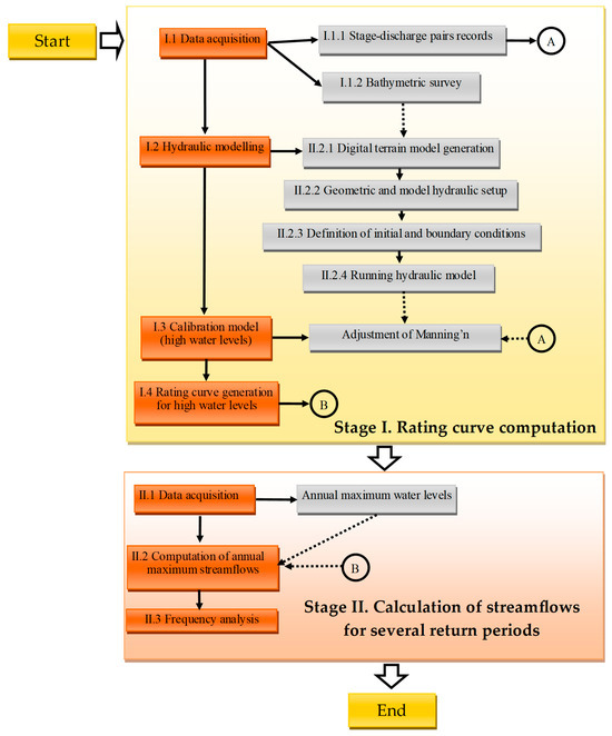
Figure 1. Proposed methodology in this study.

2.1.1. Rating Curve Computation

To develop a reliable rating curve, it is necessary to undertake the following data acquisition activities (Stage I.1):

• Stage–discharge paired records: These data points are essential, as they are used for calibration purposes. Typically, local governments have environmental agencies responsible for carrying out these measurements. The greater the number of paired records, the higher the confidence in the resulting rating curve. In Colombia, the Institute of Hydrology, Meteorology, and Environmental Studies (IDEAM, by its Spanish acronym) typically conducts several measurements at each hydrological station.
• Bathymetric survey: To develop a hydraulic model, the bathymetric data must be collected not only at the location of the hydrological station but also upstream and downstream of it.

Based on the bathymetric survey, a Digital Terrain Model (DTM) is generated (see Stage II.1) for the development of the hydraulic model. This can be produced using various tools available in current modelling software. Using this information, the model’s geometric configuration can be established, covering the area surveyed during the bathymetric campaign.

Subsequently, the initial and boundary conditions must be defined. For supercritical and subcritical flow regimes, an appropriate water level must be imposed upstream and downstream, respectively. These generally depend on engineering judgement and are subsequently verified during the calibration stage. The hydraulic model is then run for different water levels, from the reference measurement level up to high flows in the analysed river. Typically, records of stage–discharge pairs are limited to average-flow conditions. Since pair records are measured under steady-state conditions, this type of modelling is required to compute rating curves.

The governing equations of the HEC-RAS model are presented in Table 1.

Table 1. Hydraulic software for 1D modelling in HEC-RAS.

Type of Equation	Governing Equations	Equation No.	Observations	References
Energy	$Z_2+Y_2+{\displaystyle \frac{{\alpha }_2{V}_2^2}{2g}}=Z_1+Y_1+{\displaystyle \frac{{\alpha }_1{V}_1^2}{2g}}+h_e$ where, $Z$ refers to elevation of the main river inverts, $Y$ corresponds to depth of water, $V$ is the average water velocity, $\alpha$ is the velocity weighting coefficients, and $h_e$ represents the energy head loss.	$\left(1\right)$	It is applied for modelling events of gradually varied flow.	[21,22]
Momentum	${\displaystyle \frac{Q_2^2{\beta }_2}{g{A}_2}}+A_2\overline{Y_2}+\left({\displaystyle \frac{A_1+A_2}{2}}\right)L{S}_0-\left({\displaystyle \frac{A_1+A_2}{2}}\right)L\overline{S_f}={\displaystyle \frac{Q_1^2{\beta }_1}{g{A}_1}}+A_1\overline{Y_1}$ where, $\overline{S_f}$ = fiction slope, $L$ = distance between cross-sections 1 and 2, $A$ = wetted area, $S_0$ = slope of the channel, $\beta$ = momentum coefficient, and $Q$ = water discharge.	$\left(2\right)$	This equation is employed for rapidly varying flow events.

After that, the Manning’s coefficient must be adjusted in the hydraulic model to generate a rating curve that follows the trend of the recorded stage–discharge pairs, as presented in Figure 2. It highlights the importance of properly calibrating the Manning’s coefficient to fit stage–discharge measurements accurately. It is also crucial to emphasise that models based solely on exponential regression cannot account for extreme flow conditions, as they rely on mathematical equations that neglect variations in cross-sectional area at high water levels. In practice, environmental agencies are rarely able to obtain measurements during extreme events; therefore, a physically based modelling approach that explicitly accounts for changes in cross-sectional geometry is required to adequately describe the relationship between water level and discharge under such conditions.

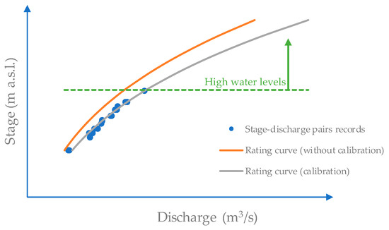
Figure 2. Rating curve generation for high water levels.

2.1.2. Calculation of Discharge for Several Return Periods

This research suggests that recorded extreme events must be interpreted in terms of high water levels using the proposed rating curve.

The estimation of annual maximum discharges for different return periods must be conducted using the probability distributions listed in Table 2 (Generalized Extreme Value (GEV) [23], Gumbel [24], Pearson type III [25], and Log-Pearson Type III [26]).

Table 2. Hydrological distributions.

Distribution	Formula	Equation No.
GEV	$f\left(Q\right)={\displaystyle \frac{1}{a}}{\left[1-{\displaystyle \frac{b}{a}}\left(Q-\mathrm{c}\right)\right]}^{{\displaystyle \frac{1}{b}}-1}\exp \left\{-{\left[1-{\displaystyle \frac{b}{a}}\left(Q-\mathrm{c}\right)\right]}^{{\displaystyle \frac{1}{b}}}\right\}$	(3)
Gumbel	$f\left(Q\right)={\displaystyle \frac{1}{\alpha }}\exp \left[-{\displaystyle \frac{Q-\mu }{\alpha }}-\exp \left(-{\displaystyle \frac{Q-\mu }{\alpha }}\right)\right]$	(4)
Pearson Type III	$f\left(Q\right)={\displaystyle \frac{1}{a\mathit{\Gamma }\left(b\right)}}{\left({\displaystyle \frac{Q-c}{a}}\right)}^{b-1} e^{\left[-\left({\displaystyle \frac{Q-c}{a}}\right)\right]}$	(5)
Log-Pearson Type III	$f\left(Q\right)={\displaystyle \frac{1}{a\mathit{\Gamma }\left(b\right)}}{\left({\displaystyle \frac{\ln Q-\mathrm{c}}{a}}\right)}^{b-1}{e}^{\left[-\left({\displaystyle \frac{\ln Q-c}{a}}\right)\right]}$	(6)

Note(s): Where, $f\left(Q\right)$ = Probability density function, $Q=$ annual maximum discharge, $a$ = scale parameter (GEV, Pearson Type III, and Log-Pearson Type III), $b$ = shape parameter (GEV, Pearson Type III, and Log-Pearson Type III), $c$ = location parameter (GEV, Pearson Type III, and Log-Pearson Type III), $\alpha$ = scale parameter (Gumbel), $\mu$ = location parameter (Gumbel).

To fit the hydrological distributions described in Table 2, the maximum likelihood and L-moment methods were used to estimate the parameters of each distribution, as shown in Table 3. These fitting methods were selected based on the adjustments reported in various investigations.

Table 3. Methods for estimating the parameters of hydrological distributions.

Method	Formula	Equation No.
Maximum likelihood	$L(\mathit{\theta })={\displaystyle \prod _{i=1}^n}{f}_Q\left(\left.Q_i\right|\mathit{\theta }\right)$	(7)
L-moments	$\left\{\begin{array}{c}\widehat{{\lambda }_1}=\widehat{{\beta }_0}\\ \widehat{{\lambda }_2}=2\widehat{{\beta }_1}-\widehat{{\beta }_0}\\ \widehat{{\lambda }_3}=6\widehat{{\beta }_2}-\widehat{{\beta }_1}+\widehat{{\beta }_0}\\ \widehat{{\lambda }_4}=20\widehat{{\beta }_3}-30\widehat{{\beta }_2}+12\widehat{{\beta }_1}-\widehat{{\beta }_0}\end{array}\right.$	(8)

Note(s): Where, $L\left(\mathit{\theta }\right)$ = likelihood function, $Q=$ annual maximum discharge, $\mathit{\theta }$ = set of parameters, $f_Q$ = hydrological density function, $n$ = number of observations, $\widehat{\lambda }$ = i L-moments, and $\beta$ = unbiased estimator.

To select the most suitable hydrological distributions, three statistical goodness-of-fit measures were employed: (i) the Chi-square test, (ii) the Kolmogorov–Smirnov test, and (iii) the Anderson–Darling test. The Chi-square test is commonly used to assess whether there is a significant difference between observed and expected discharges under a given hydrological distribution. The Kolmogorov–Smirnov and Anderson–Darling tests are used to evaluate and compare multiple hydrological distributions, with lower statistic values indicating a better agreement between the theoretical distribution and the observed data.

2.2. Study Area

This study focuses on the lower Magdalena River basin at the municipality of Magangué, Bolívar (Colombia), where the channel is classified as a lowland river due to its low energy and slope [27]. The municipality of Magangué is part of the Momposina Depression, a concave area of approximately 40,000 km² that is subject to continuous subsidence driven by the weight of sediments deposited annually during the overflows of rivers and streams [28]. Around 80% of the Caribbean region’s total wetlands are concentrated in the Momposina Depression, which is fed by four fluvial systems: the Magdalena, Cesar, Cauca, and San Jorge rivers [29].

The dataset used in this research was obtained from the hydrological station on the Magdalena River at Magangué (station code: 25027680). This station is located at latitude 528,375.25 and longitude 1,021,397.56, which is operated by IDEAM. Figure 3 presents the location of the case study.

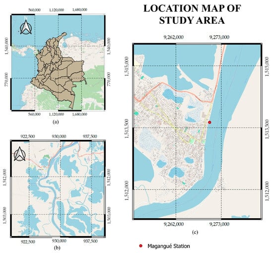
Figure 3. Location of the study area: (a) map of Colombia; (b) location of the Magangué Municipality; and (c) location of the study area.

The hydrological station has maintained a continuous record since 1973, providing a robust, long-term dataset for hydrological analysis. Over this period, considerable variability in Magdalena River discharge has been documented, with 2010 particularly notable for the highest historical discharge of 11,127 m³/s (reported by IDEAM) during the most severe rainy season to affect the country. Hydrological records at the Magangué gauging station inherently incorporate the effects of lateral inflows, direct rainfall, evaporation, baseflow, and channel losses.

The dataset comprises stage-discharge pairs (see Table 4) and annual maximum water levels (see Table 5) measured at the Magangué gauging station on the Magdalena River. All water levels are referenced to a benchmark (BM) located at an elevation of 8.051 m a.s.l.

Table 4. Stage-discharge pairs records at the Magangué gauging station on the Magdalena River.

Date	Stage (m a.s.l.)	Discharge (m3/s)
9 February 2018	13.09	4277
20 February 2019	11.39	2676
26 May 2019	14.17	5685
20 February 2020	12.03	3512
17 February 2021	12.08	3511
4 September 2021	15.17	3127

Table 5. Annual maximum water levels at the Magangué gauging station on the Magdalena River are reported by IDEAM.

Year	Water Level (m a.s.l.)	Year	Water Level (m a.s.l.)	Year	Water Level (m a.s.l.)
1973	17.01	1990	15.74	2007	17.23
1974	17.10	1991	14.59	2008	17.57
1975	17.01	1992	14.13	2009	16.92
1976	14.96	1993	15.85	2010	18.01
1977	16.00	1994	15.94	2011	17.67
1978	15.45	1995	16.37	2012	17.50
1979	16.74	1996	16.54	2013	15.05
1980	15.19	1997	14.62	2014	15.08
1981	16.94	1998	16.35	2015	13.39
1982	16.19	1999	17.21	2016	15.84
1983	14.48	2000	16.80	2017	16.18
1984	17.24	2001	15.35	2018	15.93
1985	15.52	2002	15.21	2019	15.45
1986	15.63	2003	16.50	2020	16.07
1987	16.44	2004	16.54	2021	16.86
1988	17.19	2005	17.44	2022	17.29
1989	16.39	2006	16.71	2023	17.16

Note: Water levels reported by IDEAM were converted to metres above sea level (m a.s.l.).

A bathymetric surface covering approximately 7 km of the Magdalena River was used. Along this reach, cross-sections were defined at 20 m intervals, allowing the channel profile to be captured at regular intervals. These sections accurately depict key hydraulic features, including variations in width, depth, and river curvature. Based on the surveyed bathymetry, the channel margins and centerline were delineated. This procedure enabled the construction of a geometric model that reliably reflects the natural conditions of the riverbed. Figure 4 illustrates the survey configuration, which employed an echo sounder that transmitted acoustic pulses to measure riverbed depth.

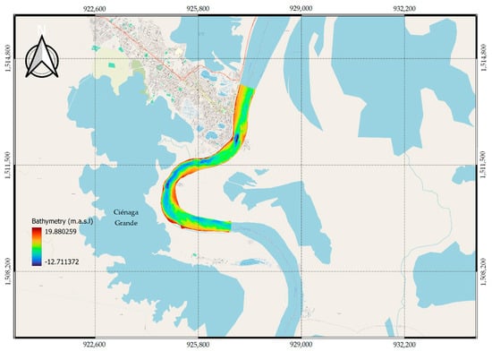
Figure 4. Bathymetry survey in the study area.

3. Results

3.1. Hydraulic Modelling

In this study, the HEC-RAS 1D (one-dimensional hydraulic model) software (Version 6.6) was used to calibrate the Manning’s coefficient for the branch at the Magangué station. The procedure begins with data acquisition and preprocessing, followed by the generation of a digital terrain model from the bathymetric survey. Subsequently, the channel geometry was modeled in HEC-RAS, and the boundary and flow-regime conditions were specified for the hydraulic simulation. For model execution, a 5 × 5 Digital Elevation Model (DEM) was provided to the software, generated from the bathymetric survey with cross-sections taken every 25 m from bank to bank. The required geometry was then defined in HEC-RAS, including the river centerline and banks, the study area, and the cross-sections. The hydraulic analysis was conducted under steady-flow conditions, assuming that flow properties—such as discharge, depth, and velocity—remain constant during the instantaneous measurements. This assumption is justified by the long time of concentration of the Magdalena River in this reach. This approach is suitable for comparing numerical results with field discharge measurements obtained under stable conditions. As the upstream boundary condition, representative unit discharges reflecting the river’s average behavior were applied. At the downstream boundary, an energy slope of 0.017% was prescribed, corresponding to the longitudinal slope of the analysed reach, which provided the best calibration at the Magangué gauging station. The flow in this river reach is governed by subcritical conditions.

To determine the values at which the Manning’s coefficient varies, the stage-discharge pairs records were analysed, as shown in Figure 5, and it was found that the coefficient ranges from 0.046 to 0.052. Then, the coefficient was calibrated over the range of hydraulic conditions represented in the dataset, and the resulting values are considered valid for the measurement zone. In this research, all available measurements were considered; however, the measurement recorded on 4 September 2021 (Table 4) was identified as an outlier and was therefore excluded from the calculations, as the reported water level was unrealistically high and inconsistent with comparable measurements.

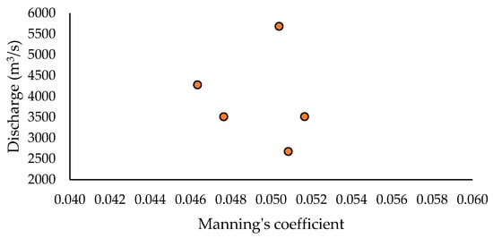
Figure 5. Characterisation of Manning’s roughness coefficient based on field measurements.

Figure 6 presents the velocity heat map derived using HEC-RAS 1D. The hydraulic modelling was performed using the entire cross-sectional geometry, including the main channel and part of the adjacent floodplains (see green lines in Figure 6), thereby representing compound-channel flow when water levels exceed bankfull conditions.

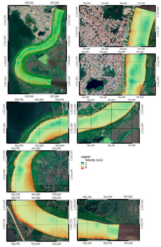
Figure 6. Plan view of the velocity contour map.

The calibration process was carried out by adjusting Manning’s roughness coefficients for the banks and the main channel, obtaining values of 0.052 and 0.046 for the channel banks and for the main river, respectively, which are applicable for high water levels and are consistent with the Manning’s coefficient evaluated for regular events (see Figure 7).

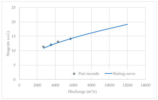
Figure 7. Rating curve for computing high water levels at the Magangué station (chainage K0+260 at the hydraulic model).

The Nash–Sutcliffe Efficiency (NSE) coefficient was adopted as a statistical measure to evaluate the accuracy of the rating curve [30]. It is beneficial for comparing observed values with those simulated by a model [31], employing the formula:

$$NSE=1-{\displaystyle \frac{{\sum }_{i=1}^n{(O_i-S_i)}^2}{{\sum }_{i=1}^n{(O_i-\overline{O})}^2}}$$

(9)

where $O_i=$ discharge obtained from the records, $S_i$ = discharge simulated using HEC-RAS, $\overline{O}$ = mean of discharge obtained from the records, and $N$ = number of observations.

An NSE of 0.92 was obtained, indicating a good fit and reliability for simulations of high water levels in the Magangué River.

The Root Mean Square Error (RMSE) was computed for the zone with available information, as expressed by:

$$RMSE=\sqrt{{\displaystyle \frac{1}{n}}\sum _{i=1}^n{(O_i-S_i)}^2}$$

(10)

For the recorded stage–discharge pairs, an RMSE of 287 m³/s was obtained. This value is considered acceptable given the order of magnitude of the measurements, which range from 2675.62 to 5688.06 m³/s, indicating a satisfactory agreement between observed and simulated discharges.

Figure 8 presents the HEC-RAS modelling results for the different water levels measured at the Magangué gauging station, showing that all levels are confined to the main channel and do not extend into the floodplain.

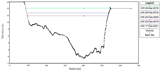
Figure 8. Water levels corresponding to the stage–discharge measurements at the cross-section of the Magangué gauging station.

3.2. Computation of Maximum Discharges for Several Return Periods

Once the HEC-RAS hydraulic model was calibrated, the annual maximum discharges were evaluated using the water-level records from the hydrometric station (see Table 5). In this regard, the rating curve shown in Figure 7 was used to estimate the annual maximum discharge, as shown in Table 6.

Table 6. Annual maximum discharge at the Magangué gauging station on the Magdalena River computed using the proposed methodology.

Year	Discharge (m3/s)	Year	Discharge (m3/s)	Year	Discharge (m3/s)
1973	9175	1990	7560	2007	9468
1974	9295	1991	6219	2008	9928
1975	9175	1992	5710	2009	9055
1976	6640	1993	7695	2010	10,536
1977	7880	1994	7806	2011	10,065
1978	7213	1995	8344	2012	9833
1979	8820	1996	8560	2013	6744
1980	6906	1997	6252	2014	6779
1981	9081	1998	8319	2015	4960
1982	8117	1999	9441	2016	7683
1983	6094	2000	8898	2017	8104
1984	9481	2001	7094	2018	7794
1985	7296	2002	6929	2019	7213
1986	7427	2003	8508	2020	7966
1987	8432	2004	8560	2021	8976
1988	9414	2005	9752	2022	9548
1989	8369	2006	8781	2023	9374

The frequency analysis was carried out using several hydrological probability distributions based on the maximum discharges listed in Table 6. As the principal aim is to model flood events (i.e., peak flows), only probability distributions explicitly suited to extreme-value analysis were considered. These distributions—Gumbel, Generalised Extreme Value (GEV), Pearson Type III, and Log-Pearson Type III—are widely used in hydrology because they reliably capture the statistical behaviour of rare and extreme events, such as river floods, enabling the estimation of peak discharges for various return periods.

Table 7 summarises the results of three goodness-of-fit tests (Kolmogorov–Smirnov, Chi-Square, and Anderson–Darling) for each distribution using two parameter estimation methods: L-moments and Maximum Likelihood. Lower test statistics indicate a better fit between the theoretical distribution and the observed data.

Table 7. Test statistic for selecting the best hydrological distribution.

Distribution	Fitting Method	Statistical Test
		Kolmogorov–Smirnov	Chi-Square	Anderson–Darling
Log-Pearson III	L-Moments	0.04	2.92	0.14
Generalized Extreme Value	L-Moments	0.05	3.71	0.13
Pearson III	L-Moments	0.05	4.49	0.17
Gumbel	L-Moments	0.14	12.33	1.62
Log-Pearson III	Maximum Likelihood	0.05	4.49	0.14
Generalized Extreme Value	Maximum Likelihood	0.05	3.31	0.15
Pearson III	Maximum Likelihood	0.05	2.92	0.19
Gumbel	Maximum Likelihood	0.11	12.73	1.13

According to the results, the Log-Pearson III distribution fitted using L-moments performs best overall. This option consistently produced the lowest values across all three statistical tests, indicating the closest agreement with the observed maximum discharges. The Generalized Extreme Value distribution using L-moments presents the second-best option. In contrast, the Gumbel distribution exhibited a poor fit for extreme flows. Overall, the results highlight the superior performance of L-moments over Maximum Likelihood.

Frequency analysis was conducted for several return periods using HEC-SSP 2.3, with the Log-Pearson III distribution fitted to L-moments, as shown in Figure 9. This software was employed because it allows the application of L-moment methods, whose usefulness has been widely demonstrated in the literature, particularly for the analysis of extreme high-magnitude events [32,33]. For a 100-year return period, the estimated peak discharge is 10,543 m³/s, whereas for a 5-year return period, it is 9308 m³/s. The 5% and 95% confidence limits are also presented, indicating that all observed annual maximum discharges fall within this interval. The observed maximum yearly discharges (blue circles) align closely with the theoretical Log-Pearson III curve, indicating an adequate representation of the flood regime at the Magangué gauging station.

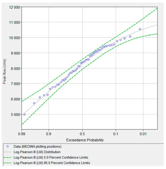
Figure 9. Frequency analysis of annual maximum discharge at the Magangué gauging station.

4. Discussion

A sensitivity analysis of annual maximum discharge was conducted for return periods ranging from 10 to 200 years, comparing IDEAM-reported values with those obtained using the proposed methodology. Table 8 summarises the annual maximum discharges published by IDEAM for the Magangué gauging station. These values are derived from a rating curve developed using an exponential regression applied to the available stage–discharge records.

Table 8. Annual maximum discharge at the Magangué gauging station on the Magdalena River, as reported by IDEAM.

Year	Discharge (m3/s)	Year	Discharge (m3/s)	Year	Discharge (m3/s)
1973	8531	1990	6661	2007	9025
1974	8849	1991	5878	2008	9532
1975	8483	1992	5743	2009	8502
1976	7098	1993	8084	2010	11,127
1977	8145	1994	7661	2011	10,503
1978	7371	1995	7510	2012	10,192
1979	8890	1996	7824	2013	6350
1980	7325	1997	5192	2014	6384
1981	9110	1998	7474	2015	4299
1982	8568	1999	8992	2016	7455
1983	6587	2000	8292	2017	7983
1984	8305	2001	6270	2018	7738
1985	6814	2002	5891	2019	7141
1986	7666	2003	7743	2020	7913
1987	8335	2004	7824	2021	8920
1988	9086	2005	9364	2022	9300
1989	8426	2006	8130	2023	7832

Based on the IDEAM discharge series (Table 8), a frequency analysis was conducted using the Pearson III distribution with L-moments to estimate peak discharges for several return periods, since it performed best in the statistical tests (Kolmogorov–Smirnov, Chi-Square, and Anderson–Darling). Table 9 presents a comparison between the maximum discharge for each return period, contrasting IDEAM’s values with those computed using the proposed methodology.

Table 9. Comparison of annual maximum discharge and water level for different return periods using IDEAM data and the methodology proposed in this research.

Return Period (Years)	Annual Maximum Discharge (m3/s)		Ratio
	IDEAM	Proposed Methodology
2	7958	8300	4.1%
5	9010	9308	3.2%
10	9521	9750	2.3%
20	9925	10,066	1.4%
50	10,358	10,370	0.1%
100	10,636	10,543	−0.9%
200	10,881	10,680	−1.9%

For return periods ranging from 2 to 50 years, the proposed methodology yields higher discharge estimates than those derived from the IDEAM frequency analysis. The relative increase ranges from approximately 4.1% for the 2-year event (7958 versus 8300 m³/s) to around 1.4–3.2% for the 5- to 20-year events. For the 50-year return period, a marginal difference of around 0.1% is observed. In contrast, for more extended return periods (100–200 years), the methodology yields lower discharge values than IDEAM. The difference remains approximately 0.9% lower for the 100-year event and approximately 1.9% lower for the 200-year event. It is important to emphasise that the Magdalena River is considerably less sensitive to the rating curve than many other watercourses, as reflected by the relatively low discharge ratios across return periods (for example, a ratio of only 1.08 between the 100- and 10-year events).

The present study assumes that the channel cross-sectional geometry remains constant over time, despite the occurrence of erosion and sedimentation processes. Steady-state flow conditions were adopted for the derivation of the rating curve.

The implemented one-dimensional HEC-RAS model does not account for interactions with the Ciénaga Grande located near the Magdalena River (See Figure 4), which can influence flood propagation and flow attenuation during extreme events.

5. Conclusions

This research presents a methodology for deriving rating curves, which is crucial for interpreting maximum water levels that are often not directly measured. The proposed approach is based on paired stage–discharge records, used in conjunction with a hydraulic model to compute annual maximum discharges. This method overcomes a key limitation of traditional exponential regressions, which are unable to adequately represent extreme flow conditions because they fail to capture cross-sectional variation at elevated stages. A detailed frequency analysis must then be carried out to identify the most appropriate hydrological distribution for estimating discharges across a range of return periods. For the case study at the Magangué station on the Magdalena River in Colombia, the Log-Pearson Type III distribution, fitted using L-moments, yielded the best overall performance across multiple goodness-of-fit criteria. Accordingly, a sensitivity analysis of maximum water levels was carried out for return periods between 2 and 200 years, showing discrepancies of up to 4.2% relative to the traditional exponential regression method.

Engineering projects should adopt this methodology when interpreting annual maximum discharges to avoid over- and underestimation of design discharges across different return periods.

References

- Hodson, T.O.; Doore, K.J.; Kenney, T.A.; Over, T.M.; Yeheyis, M.B. Ratingcurve: A Python Package for Fitting Streamflow Rating Curves. Hydrology 2024, 11, 14. [Google Scholar] [CrossRef]
- Martin, I.; Salcedo, R.; Font, R. Flujo Interno de Fluidos Incomprensibles y Comprensibles. In Mecanica de Fluidos; Universidad de Alicante: San Vicente del Raspeig, Spain, 2011; pp. 15–16. [Google Scholar]
- Ali, G.; Maghrebi, M.F. A Robust Approach for the Derivation of Rating Curves Using Minimum Gauging Data. J. Hydrol. 2023, 623, 129609. [Google Scholar] [CrossRef]
- Rojas, M.; Quintero, F.; Young, N. Analysis of Stage–Discharge Relationship Stability Based on Historical Ratings. Hydrology 2020, 7, 31. [Google Scholar] [CrossRef]
- Al-abadi, A.M. Modeling of Stage—Discharge Relationship for Gharraf River, Southern Iraq Using Backpropagation Artificial Neural Networks, M5 Decision Trees, and Takagi—Sugeno Inference System Technique: A Comparative Study. Appl. Water Sci. 2014, 6, 407–420. [Google Scholar] [CrossRef]
- Goel, A.; Pal, M. Stage-discharge modeling using support vector machines. Int. J. Eng. 2012, 25, 1–9. [Google Scholar] [CrossRef]
- Kuhanestani, P.K.; Bomers, A.; Booij, M.J.; Hulscher, S.J.M.H. Hydraulic River Model Calibration and Validation for Comprehensive Hydrograph Simulation: Evaluating Accuracy across Discharge Ranges. J. Hydrol. 2025, 660, 133210. [Google Scholar] [CrossRef]
- Kong, L.; Li, Y.; Yuan, S.; Li, J.; Tang, H.; Yang, Q.; Fu, X. Research on Water Level Forecasting and Hydraulic Parameter Calibration in the 1D Open Channel Hydrodynamic Model Using Data Assimilation. J. Hydrol. 2023, 625, 129997. [Google Scholar] [CrossRef]
- Costabile, P.; Costanzo, C.; Ferraro, D.; Barca, P. Is HEC-RAS 2D Accurate Enough for Storm-Event Hazard Assessment? Lessons Learnt from a Benchmarking Study Based on Rain-on-Grid Modelling. J. Hydrol. 2021, 603, 126962. [Google Scholar] [CrossRef]
- Pappenberger, F.; Beven, K.; Horritt, M.; Blazkova, S. Uncertainty in the Calibration of Effective Roughness Parameters in HEC-RAS Using Inundation and Downstream Level Observations. J. Hydrol. 2005, 302, 46–69. [Google Scholar] [CrossRef]
- Bruno, L.S.; Mattos, T.S.; Oliveira, P.T.S.; Almagro, A.; Rodrigues, D.B.B. Hydrological and Hydraulic Modeling Applied to Flash Flood Events in a Small Urban Stream. Hydrology 2022, 9, 223. [Google Scholar] [CrossRef]
- Santos, R.; Cubillos, C.; Vargas, A. Modelación Hidráulica de Un Sector de Río Caudaloso Con Derivaciones Empleando HEC-RAS. In Avances en Recursos Hidráulicos; Universidad Nacional de Colombia: Medellín, Colombia, 2008; pp. 43–54. [Google Scholar]
- Acuña, G.J.; Ávila, H.; Canales, F.A. River Model Calibration Based on Design of Experiments Theory. A Case Study: Meta River, Colombia. Water 2019, 11, 1382. [Google Scholar] [CrossRef]
- Vatanchi, S.M.; Maghrebi, M.F. Estimating streamflow by an innovative rating curve model based on hydraulic parameters. Environ. Earth Sci. 2024, 83, 266. [Google Scholar] [CrossRef]
- McMahon, T.A.; Peel, M.C. Uncertainty in Stage–Discharge Rating Curves: Application to Australian Hydrologic Reference Stations Data. Hydrol. Sci. J. 2019, 64, 255–275. [Google Scholar] [CrossRef]
- Kumar, V.; Sen, S. Rating Curve Development and Uncertainty Analysis in Mountainous Watersheds for Informed Hydrology and Resource Management. Front. Water 2023, 5, 1323139. [Google Scholar] [CrossRef]
- Negatu, T.A.; Zimale, F.A.; Steenhuis, T.S. Establishing Stage–Discharge Rating Curves in Developing Countries: Lake Tana Basin, Ethiopia. Hydrology 2022, 9, 13. [Google Scholar] [CrossRef]
- Baruah, A.; Spies, R.; Devi, D.; Cohen, S.; Aristizabal, F.; Nikrou, P.; Tian, D.; Pruitt, C. Predicting Synthetic Rating Curve Adjustment Factors with Explainable Machine Learning for Enhancing the United States Operational Flood Inundation Mapping Framework. J. Hydrol. 2025, 662, 134086. [Google Scholar] [CrossRef]
- Salgado, J.; Jaramillo-Monroy, C.; Link, A.; Lopera-Congote, L.; Velez, M.I.; Gonzalez-Arango, C.; Yang, H.; Panizzo, V.N.; McGowan, S. Riverine Connectivity Modulates Elemental Fluxes through a 200- Year Period of Intensive Anthropic Change in the Magdalena River Floodplains, Colombia. Water Res. 2025, 268, 122633. [Google Scholar] [CrossRef]
- Rivillas-Ospina, G.; Díaz, K.; Gutiérrez, R.R.; Berrío, Y.; Doria, R.; Felizzola, M. Numerical Simulation and Application of Nature Based Solutions to Solve Bank Erosion in Hydrosystems. Ecohydrol. Hydrobiol. 2024, 25, 556–572. [Google Scholar] [CrossRef]
- Brunner, G. HEC-RAS, River Analysis System Hydraulic Reference Manual; Version 6.0 Beta; US Army Corps of Engineers—Hydrologic Engineering Center (HEC): Davis, CA, USA, 2020. [Google Scholar]
- Teleszewski, T.J. Experimental Investigation of the Kinetic Energy Correction Factor in Pipe Flow. In Proceedings of the 10th Conference on Interdisciplinary Problems in Environmental Protection and Engineering EKO-DOK 2018, E3S Web of Conferences, Polanica-Zdrój, Poland, 16–18 April 2018; EDP Sciences: Les Ulis, France, 2018; Volume 44, pp. 1–6. [Google Scholar] [CrossRef]
- Provost, S.B.; Saboor, A.; Cordeiro, G.M.; Mansoor, M. On the Q-Generalized Extreme Value Distribution. REVSTAT-Stat. J. 2018, 16, 45–70. [Google Scholar] [CrossRef]
- Wang, J.; Qin, S.; Jin, S.; Wu, J. Estimation Methods Review and Analysis of Offshore Extreme Wind Speeds and Wind Energy Resources. Renew. Sustain. Energy Rev. 2015, 42, 26–42. [Google Scholar] [CrossRef]
- Singh, V.P. Pearson Type III Distribution. In Entropy-Based Parameter Estimation in Hydrology; Springer: Dordrecht, The Netherlands, 1998; pp. 231–251. [Google Scholar] [CrossRef]
- Ulusoy, I.C.; Erdik, T. An Investigation of Prospective Current Power Generation with the Log Pearson Type 3 Distribution in the Upper Layer in the Vicinity of the Northern Bosphorus. Sustain. Energy Technol. Assess. 2021, 47, 101363. [Google Scholar] [CrossRef]
- Díaz, E.; Ollero, A. Metodologia Para La Clasificación Geomorfológica De Los Cursos Fluviales De La Cuenca Del Ebro. Geographicalia 2005, 47, 23–45. [Google Scholar] [CrossRef]
- Alzate, C.; Turbay, S. La Fauna de La Depresión Momposina; Lealon: Los Angeles, CA, USA, 2020. [Google Scholar]
- Herrera, L.; Sarmiento, G.; Romero, F.; Botero, P.; Berrio, J.C. Evolución Ambiental De La Depresión Momposina (Colombia) Desde El Pleistoceno Tardío a Los Paisajes Actuales. Geol. Colomb. 2001, 26, 95–121. [Google Scholar]
- Coy, M.L. Ajuste Y Validación Del Modelo Precipitación-Escorrentía Gr2M Aplicado a La Subcuenca Nevado; Universidad Santo Tomas: Bogotá, Colombia, 2017; pp. 1–11. [Google Scholar]
- Krause, P.; Boyle, D.P.; Bäse, F. Comparison of Different Efficiency Criteria for Hydrological Model Assessment. Adv. Geosci. 2005, 5, 89–97. [Google Scholar] [CrossRef]
- Anghel, C.G. Revisiting the Use of the Gumbel Distribution: A Comprehensive Statistical Analysis Regarding Modeling Extremes and Rare Events. Mathematics 2024, 12, 2466. [Google Scholar] [CrossRef]
- Chen, X.; Shao, Q.; Xu, C.Y.; Zhang, J.; Zhang, L.; Ye, C. Comparative Study on the Selection Criteria for Fitting Flood Frequency Distribution Models with Emphasis on Upper-Tail Behavior. Water 2017, 9, 320. [Google Scholar] [CrossRef]
Disclaimer/Publisher’s Note: The statements, opinions and data contained in all publications are solely those of the individual author(s) and contributor(s) and not of MDPI and/or the editor(s). MDPI and/or the editor(s) disclaim responsibility for any injury to people or property resulting from any ideas, methods, instructions or products referred to in the content. |
© 2026 by the authors. Licensee MDPI, Basel, Switzerland. This article is an open access article distributed under the terms and conditions of the Creative Commons Attribution (CC BY) license.