Predicting Offshore Oil Slick Formation: A Machine Learning Approach Integrating Meteoceanographic Variables

Abstract

The presence of oil slicks in the ocean presents significant environmental and regulatory challenges for offshore oil processing operations. During primary oil–water separation, produced water is discharged into the ocean, carrying residual oil, which is measured using the total oil and grease (TOG) method. The formation and spread of oil slicks are influenced by metoceanographic variables, including wind direction (WD), wind speed (WS), current direction (CD), current speed (CS), wind wave direction (WWD), and peak period (PP). In Brazil, regulatory limits impose sanctions on companies when oil slicks exceed 500 m in length, making accurate prediction of their occurrence and extent crucial for offshore operators. This study follows three main stages. First, the performance of five machine learning classification algorithms is evaluated, selecting the most efficient method based on performance metrics from a Brazilian company’s oil slick database. Second, the best-performing model is used to analyze the influence of metoceanographic variables and TOG levels on oil slick occurrence and detection probability. Finally, the third stage examines the extent of detected oil slicks to identify key contributing factors. The prediction results enhance decision-support frameworks, improving monitoring and mitigation strategies for offshore oil discharges.

1. Introduction

Once extracted from the ocean, crude oil undergoes primary processing to separate the oil, water, and gas phases. It is estimated that tens of millions of barrels of water are produced daily worldwide during this process, posing a significant challenge for the oil industry in terms of water treatment [1]. Produced water often contains oil and grease, and elevated levels of these compounds can harm the marine environment when discharged back into the ocean. Several methods are available to evaluate the amount of oil in the produced water, including spectrophotometric, gravimetric, and calorimetric techniques. Therefore, monitoring the total oil and grease (TOG) levels is essential to ensure environmental compliance. In Brazil, the National Council for the Environment (CONAMA) regulates the discharge of produced water into the ocean through Resolution 393/2007 [2]. According to these guidelines, water discharge must meet specific TOG limits and must not alter the sea’s characteristics beyond the mixing zone, defined as a 500-m radius from the disposal point. Oil slicks exceeding this limit can result in penalties for primary oil processing companies. Satellite and aerial images can capture these oil slicks depending on their extent and the presence of meteoceanographic variables.

Predicting the occurrence of oil slicks through TOG metric and meteoceanographic variables is a valuable result when exploring oil offshore. This was approached in this study using various machine learning classification methods. Multivariate techniques were also employed to mitigate the effects of variable correlation, along with central composite and factorial designs and advanced classification algorithms.

Given these considerations, this study aims to evaluate the relationship between TOG levels and meteoceanographic variables concerning oil slick classification and extent. This study incorporates spectrophotometric TOG measurements and considers the following meteoceanographic factors: wind direction (WD, °), wind speed (WS, m/s), current direction (CD, °), current speed (CS, m/s), wind wave direction (WWD, °), and peak period (PP, s).

The remainder of this paper is structured as follows. Section 2 provides an overview of produced water on offshore oil slick formation, the role of meteoceanographic variables, and machine learning approaches on oil slicks classification and extension. Section 3 details the materials and methods. Section 4 presents and discusses the results, and Section 5 concludes with the key findings and recommendations. A more theoretical overview of the machine learning techniques is in Appendix A.

2. Background and Literature Review

2.1. The Problem of Oil Slick Formation Caused by Produced Water from Marine Offshore Oil Exploration

The formation of oil slicks due to produced water in offshore oil exploration is a significant environmental concern. Produced water is a byproduct of oil and gas extraction, consisting of water that comes from underground reservoirs, along with hydrocarbons. This water often contains residual oil, chemicals, heavy metals, and other contaminants. When discharged into the ocean without proper treatment, the oil content in produced water can accumulate on the surface, leading to the formation of slicks that spread over large areas, affecting marine ecosystems and coastal environments.

The environmental impact of these oil slicks is severe. Marine organisms, including fish, seabirds, and mammals, are particularly vulnerable, as oil exposure can damage their skin, feathers, and respiratory systems. Oil slicks also block sunlight from penetrating the water surface, reducing photosynthesis in marine plants and phytoplankton, which are crucial for the ocean’s food chain. Additionally, the accumulation of oil in seabeds and coastal regions disrupts the ecological balance, causing long-term harm to biodiversity. The presence of toxic substances in produced water can further contribute to bioaccumulation, affecting not only marine life but also human populations that depend on seafood.

The National Oceanic and Atmospheric Administration (NOAA) classifies oil slick formation into five categories based on thickness. These range from the Sheen class, a thin, nearly transparent layer, to Emulsified Oil (Mousse), a dense water-in-oil mixture. Intermediate categories include Metallic, Transitional Dark, and Dark (True) Color, with increasing thickness and opacity [3].

Economically, the consequences of oil slicks from produced water discharge are significant. Fisheries suffer from declining fish stocks due to contamination, impacting livelihoods and food supply. Coastal tourism is also affected, as polluted beaches deter visitors, leading to financial losses for local businesses. Furthermore, cleaning up oil slicks and mitigating environmental damage requires costly and time-consuming efforts, placing an additional burden on governments and industries.

To address this issue, stringent environmental regulations and advanced treatment technologies are essential. Produced water should undergo thorough separation processes to remove oil and harmful substances before being discharged. Techniques such as mechanical separation, chemical treatment, and biological filtration can significantly reduce the oil content in produced water. Additionally, reinjection of produced water into underground formations is a sustainable method to prevent marine pollution. Implementing strict monitoring and enforcement of discharge standards can help minimize the risk of oil slick formation, ensuring the protection of marine ecosystems and sustainable offshore oil exploration.

2.2. TOG as a Method to Monitor Produced Water from Marine Offshore Oil Exploration

Total oil and grease (TOG) analysis is a widely used method for monitoring produced water in marine offshore oil exploration. The TOG measurement is crucial for assessing the concentration of oil and grease in produced water to ensure compliance with environmental regulations and minimize the impact on marine ecosystems. A TOG analysis involves quantifying the total concentration of petroleum hydrocarbons, fats, oils, and other organic compounds present in water samples. The most common methods for TOG measurement include solvent extraction, followed by infrared spectroscopy or gravimetric analysis. In infrared spectroscopy, the extracted hydrocarbons are analyzed based on their absorption of infrared light at specific wavelengths, providing a precise measurement of the oil content. Gravimetric analysis, on the other hand, involves evaporating the solvent and weighing the residual oil to determine the concentration. Both techniques are effective in detecting even trace amounts of oil in produced water. Monitoring the TOG in produced water is essential for environmental protection and regulatory compliance. Most countries impose strict discharge limits on offshore oil and gas operations to prevent excessive oil pollution. Regular TOG measurements allow operators to ensure that produced water treatment systems, such as oil–water separators, filtration units, and chemical treatments, are functioning effectively. If the TOG levels exceed permissible limits, corrective actions, such as improving separation efficiency or reinjecting produced water into underground reservoirs, may be required. In addition to regulatory compliance, TOG monitoring helps oil and gas companies optimize water treatment processes and reduce environmental risks. By continuously tracking oil content, operators can detect leaks, equipment malfunctions, or inefficiencies in separation systems, preventing uncontrolled discharges into the marine environment. Advanced technologies, such as online TOG analyzers, provide real-time monitoring, enabling an immediate response to fluctuations in oil content and enhancing operational efficiency. Overall, TOG analysis plays a critical role in managing produced water in offshore oil exploration. By ensuring accurate monitoring and adherence to environmental regulations, it helps protect marine life, maintain water quality, and promote sustainable oil and gas operations.

2.3. The Role of Meteoceanographic Variables in Oil Slick Formation

The meteoceanographic variables considered herein are wind direction (WD, °), wind speed (WS, m/s), current direction (CD, °), current speed (CS, m/s), wind wave direction (WWD, °), and peak period (PP, s). These variables play a crucial role in the formation, movement, and dispersion of oil slicks in marine environments. They significantly influence how oil spreads and behaves after a spill or discharge. Considering these variables is essential for predicting oil slick trajectories, improving spill response strategies, and minimizing environmental damage.

Wind is one of the most important factors affecting oil slick formation and dispersion. Strong winds can break up the slick into smaller patches, increasing the rate of evaporation and dispersion, while calm conditions allow the oil to accumulate and form thicker layers on the surface. The wind-driven transport of oil occurs at approximately 3–4% of the wind speed, meaning that the slick moves in the direction of prevailing winds, often leading to coastal contamination if the wind pushes oil toward the shore. The percentage represents a proportional factor used in oil spill modeling to estimate the effect of wind on oil transport. The exact value may vary depending on environmental conditions, such as water currents and oil properties. For example, if the wind speed is 10 m/s, the oil slick is expected to move at 0.3 to 0.4 m/s

Ocean currents also play a significant role in oil slick movement. Surface currents can transport oil over long distances, spreading contamination across a wider area. In regions with strong tidal influences, oil slicks may be carried back and forth, prolonging their presence in a particular area and increasing environmental exposure. Additionally, upwelling and downwelling processes can affect oil distribution by mixing it vertically within the water column, making cleanup efforts more challenging.

Wave action influences oil slick thickness and breakup. Large waves tend to break the slick into smaller droplets, which can become suspended in the water column and undergo natural degradation. However, in rough seas, oil can mix with water to form emulsions, such as “chocolate mousse”, which are more persistent and difficult to clean. Calm waters, on the other hand, allow the slick to remain on the surface, leading to greater potential for coastal contamination.

It is worth mentioning that sea surface temperature affects the physical properties of oil, such as viscosity and evaporation rate, while atmospheric pressure and weather systems also contribute to oil slick dynamics. In this study, these variables will be considered as noise variables and will not be included in the models.

The findings in the recent literature on the role of meteoceanographic variables in oil slick formation are abundant and serve as the foundation for justifying the machine learning model implemented in this study. Some key findings are outlined below.

The interaction between wind and current directions plays a significant role in determining the movement and spread of oil slicks on the ocean surface. When wind and current directions are nearly opposite, their opposing forces can counteract each other, leading to reduced spreading of the oil. Conversely, when the wind direction is approximately perpendicular to the current, it can promote lateral spreading of the oil, resulting in a wider slick that covers more area. This lateral dispersion may, however, limit the along-current spread of the oil, depending on the thickness of the oil layer. These dynamics are crucial for accurately predicting oil spill trajectories and implementing effective response strategies [4,5,6,7,8,9,10].

Wind speed significantly influences the behavior and dispersion of oil slicks on the ocean surface. At lower wind speeds, wind can promote the spreading and elongation of oil slicks, with the extent and direction of spread depending on the wind’s alignment with ocean currents and their relative velocities. However, as wind speeds increase, the dynamics change notably. Higher wind speeds lead to the formation of breaking waves, which enhance the natural dispersion of oil. These breaking waves can fragment the oil slick into smaller droplets, which are then mixed into the upper layers of the ocean. Once dispersed as fine droplets, especially those smaller than a certain size threshold, the oil is less likely to resurface, effectively reducing the surface slick’s extent. This process results in shorter and smaller visible slicks on the water surface. Considering this relationship between wind speed and oil dispersion is crucial for accurately predicting oil spill behavior and implementing effective response strategies [6,11,12].

The relationship between wind conditions and wave parameters is crucial in understanding the dispersion of oil slicks on the ocean surface. Wind speeds above 7 m/s can dissipate an oil slick, whereas stronger currents often generate more extensive slicks. Wind-generated waves are not instantaneous; there is a temporal lag between changes in wind speed and direction and the corresponding adjustments in wave characteristics, such as direction and peak period. This lag means that wave parameters can serve as indicators of past wind conditions. During periods of decreasing (waning) wind speeds, existing waves, having been generated by stronger winds, may remain larger than what the current wind speeds would typically produce. This discrepancy can lead to greater dispersion of surface oil slicks than expected based solely on the present wind conditions. Conversely, during periods of increasing (waxing) wind speeds, the sea state may not yet have adjusted to the new wind conditions, resulting in smaller waves than the current winds would eventually generate. Therefore, to accurately predict oil slick behavior, it is essential to consider the relative orientations and magnitudes of wind and current, as well as the temporal evolution of wave parameters. By integrating these factors, one can develop a more predictive understanding of oil slick dispersion dynamics [8,13,14,15,16,17].

2.4. Machine Learning on Oil Slick Classification and Extension

The occurrence and extension of oil slicks can be understood as a function of meteoceanographic variables and total oil and grease (TOG) metrics. Oil slick formation refers to the initial appearance of an oil layer on the water surface, while oil slick extension describes how the slick spreads over time and space. Both processes are influenced by a combination of environmental factors and operational discharges, making accurate prediction essential for effective spill management.

This regression model can be implemented using machine learning techniques, such as linear regression, random forests, or deep learning, to predict oil slick behavior based on real-time environmental and operational data.

In this function, oil slick formation refers to the initial appearance of an oil layer on the water surface, while oil slick extension describes how the slick spreads over time and space.

Machine learning (ML) offers a powerful approach to modeling the complex, nonlinear relationships between these factors and predicting oil slick behavior. By training on historical and real-time data, ML algorithms models can estimate the probability of oil slick formation under specific conditions. Furthermore, these models can forecast the trajectory and spread of existing slicks, providing crucial information for spill response efforts. Integrating ML with remote sensing, satellite imagery, and ocean monitoring systems enables offshore operators to enhance oil spill prevention strategies, reducing both environmental impact and economic losses. In this study, five commonly applied machine learning methods were selected: random forest (RF), k-nearest neighbors (KNN), artificial neural network multi-layer perceptron (MLP), logistic regression (LR), and support vector machine (SVM); these are presented in Appendix A. Some recent studies on oil slicks using a machine learning approach can be found in [18,19,20,21].

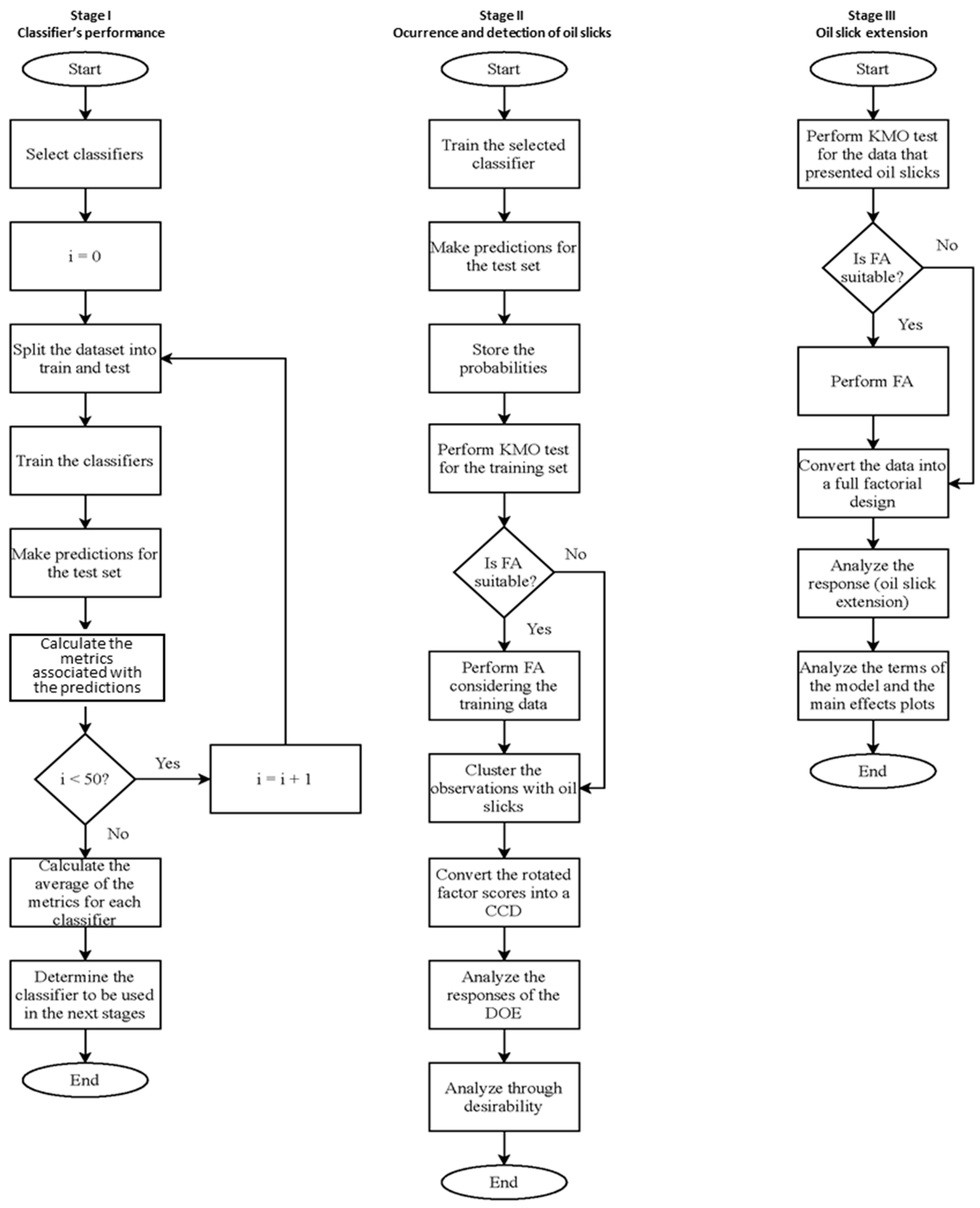
3. Materials and Methods

The dataset used in this study was collected between April 2018 and August 2020 from an offshore platform involved in primary oil processing in Brazil. It consists of 300 observations, evenly divided between two classes: 150 observations without an oil slick exceeding 500 m in length (classified as class 0) and 150 observations with such an oil slick (classified as class 1).

Figure 1 presents the classification of data based on the presence or absence of an oil slick, as a function of the predictor variables of WD, WSD, CS, WWD, PP, and TOG, showing that the problem is not a linear classification problem. Therefore, it is more suitable for machine learning models that account for non-linearity between predictor variables and the binary response, defined here as the occurrence or not of oil slicks.

Another response variable assessed in this study was the extent of the oil slick, measured in nautical miles for the 150 cases where such features were detected. It is worth noting that the detection of an oil slick is conducted via satellite, while meteoceanographic variables are measured by the Center for Weather Forecasting and Climate Studies (Centro de Previsão de Tempo e Estudos Climáticos—CPTEC). Additionally, TOG measurements are obtained through a spectrophotometric method, allowing multiple readings throughout the day to enable proactive decision-making by platform managers.

Satellites detect oily features in the ocean using optical and radar sensors, with synthetic aperture radar (SAR) being one of the most effective methods. SAR sends microwave pulses to the sea surface and measures the reflected signal, with oil reducing surface roughness, creating dark regions in SAR images. A key advantage of SAR is its ability to operate in all weather conditions, but false positives can occur due to thermal fronts, algal blooms, and calm seas.

To verify satellite detections, vessels and aircraft are deployed. Aircraft equipped with optical, infrared, and radar sensors capture high-resolution images and provide near real-time data, while drones assist in monitoring smaller areas. Vessels collect water and oil samples to determine the oil type, degradation, and origin.

The integration of satellite, aerial, and maritime data enhances oil spill detection and response, reducing uncertainties and enabling rapid action. This combined approach was used in this study to accurately classify oil slick formation.

In addition, the historical data of meteoceanographic variables were obtained from CPTEC and cross-checked with meteorological stations on the platform itself to mitigate bias. Additionally, through a data mining process, other variables with ambiguous data were discarded to ensure a reliable database.

The methodology adopted in this study encompasses three main stages. The first stage involves evaluating the performance of five classification algorithms: RF, KNN, MLP, BLR, and SVM, as mentioned before. In the second stage, the influence of meteoceanographic variables and TOG levels on the probability of oil slick occurrence and detection (P_os) is analyzed. Finally, the third stage examines the extent of the detected oil slick to identify contributing factors. Figure 2 illustrates the methodological flowchart, detailing the steps undertaken in this research.

I.

Classifiers’ performance

The initial objective of this study was to compare various classifiers to predict the probability of occurrence and detection of an oil slick. The first step involved defining the classifiers to be employed and configuring the parameters associated with each algorithm. For a robust comparison, the training and testing datasets were partitioned into 50 distinct configurations, ensuring that the class proportions remained consistent across both sets.

Once the classifiers were selected, the models were trained and tested using all the defined configurations. Performance metrics, including accuracy (Ac), specificity (Sp), and sensitivity (Sn), were computed according to Equation (1), Equation (2), and Equation (3), respectively. True positives (TP) and true negatives (TN) represent the correct classifications, while false positives (FP) and false negatives (FN) represent classification errors. The average values of these metrics were extracted for comparative purposes.

Based on the comparative analysis, the classifier that achieved the best performance according to the averaged metrics was selected for further use in the next stage of the study. This systematic approach ensures the selection of the most effective method for predicting oil slick occurrence and detection.

$$A_{cc}={\displaystyle \frac{TP+TN}{TP+TN+FP+FN}}$$

(1)

$$S_p={\displaystyle \frac{TN}{TN+FP}}$$

(2)

$$S_n={\displaystyle \frac{TP}{TP+FN}}$$

(3)

II.

Occurrence and detection of an oil slick

The selected method was applied to model the training data and generate predictions for the test set. The probabilities of oil slick occurrence and detection were stored for further analysis. A crucial step is evaluating the suitability of the training data for factor analysis. If the data follow a multivariate normal distribution, the Bartlett test of sphericity can be used to test the hypothesis that the variables are uncorrelated. However, given that the data in this study did not exhibit a multivariate normal distribution, the Kaiser–Meyer–Olkin (KMO) sampling adequacy measure was employed. Values ranging from 0.5 to 1.0 for this index indicate that factor analysis is appropriate. Factor analysis is recommended if at least one of these tests yields a favorable result.

If factor analysis is deemed appropriate, the rotated factor scores are stored and subsequently treated as predictor variables. The training set was divided into two clusters: one containing observations where oil slick occurrence and detection were recorded, and another with observations without such occurrences. The input data were then transformed into a response surface array based on the central composite design (CCD) to assess the main effects, interactions, and quadratic effects of the factors that represent the original variables.

Modeling the probabilities involved selecting the significant terms from the model. Given the potential significance of interaction and quadratic terms, relying solely on main effects analysis could lead to inaccurate conclusions. Therefore, an optimization algorithm was used to capture the complete spectrum of variable effects, ensuring a comprehensive understanding of the relationships and dependencies within the data.

III.

Oil slick extension

For the data subset where the oil slick was detected and its extension measured, the suitability of conducting a factor analysis was reassessed. However, the Kaiser–Meyer–Olkin (KMO) test did not yield values greater than 0.5 for most variables, indicating that factor analysis was not appropriate. Consequently, the predictors were converted into a full factorial design for analysis.

The choice to adopt a full factorial design was driven by the observation that including quadratic effects and interactions did not enhance the model’s quality. On the contrary, these additions led to a decrease in the adjusted coefficient of determination ($R_{adj}^2$), indicating a reduction in model fit efficiency. Therefore, a simpler model structure was maintained to ensure more accurate and robust predictions.

4. Results

4.1. Classifiers’ Performance

For this article, five commonly applied methods were selected, namely, RF, KNN, MLP, LR, and SVM. We ran 50 different training and test sets using the kfold.split function available in Python (https://www.python.org) with 535 observations for training and 60 for testing. Consequently, 50 different models were created for each of these methods, so that the accuracy of each one was computed at each step and the average was stored.

Table 1. Parametrization and precision metrics for the methods as defined by equations (1–3).

Machine Learning Algorithm	Main Parameters	Acc	Sp	Sn
RF	Estimators = 150 Max features = 3	0.77	0.73	0.82
KNN	k = 5	0.74	0.65	0.84
MLP	Number of hidden layers = 2 Number of units = 4 Activation function = Relu Solver = LBFGS α = 0.05 Learning rate = invscaling	0.71	0.68	0.76
BLR	Link function = logit	0.74	0.70	0.80
SVM	Kernel = RBF γ = 0.1 C = 1	0.75	0.65	0.85

shows the methods used, their parameterization, and the metrics obtained (on average) for the test set.

The random forest (RF) algorithm demonstrated the best performance among the evaluated methods, as depicted in Figure 3. As a result, it was selected for use in Section 4.2. To gain a deeper understanding of the influence of predictor variables on the occurrence and detection of an oil slick, the feature importance graph generated by the RF model was analyzed and stored. This graph provides valuable insights into the contribution of each variable to the prediction process, supporting a more informed interpretation of the model’s outcomes.

4.2. Occurrence and Detection of an Oil Slick

Maintaining the same proportion for the training and test sets as previously mentioned, the random forest (RF) model yielded the confusion matrix presented in

Table 2. Confusion matrix for the random forest model.

		Prediction
		Class 0	Class 1
Actual	Class 0	12	2
	Class 1	1	15

. This matrix provides valuable information regarding the classification performance, including the number of true positives, true negatives, false positives, and false negatives, allowing a comprehensive evaluation of the model’s predictive accuracy.

The feature importance graph for the RF model, which highlights the contribution of each predictor variable to the classification task, is depicted in Figure 4. Additionally, Figure 5 shows the receiver operating characteristic (ROC) curve, which illustrates the model’s ability to distinguish between classes by plotting the true positive rate against the false positive rate at various threshold settings. If we have a model that predicts oil slicks (positive) or no oil slicks (negative) using satellite images, the model gives a probability score. When setting different thresholds, a lower threshold implies more oil slicks detected (higher true positive rate), but also more false alarms (higher false positive rate). A higher threshold implies fewer false alarms but also misses some real oil slicks. Plotting the true positive rate (y-axis) vs. false positive rate (x-axis) for different thresholds forms the ROC curve. The area under the curve (AUC) serves as a key metric for evaluating the model’s classification performance. The AUC represents the overall performance of the model in distinguishing between oil slicks and non-oil slicks. A higher AUC (closer to 1.0) means the model is excellent at detecting oil slicks while minimizing false alarms. An AUC of 0.5 indicates the model is no better than random guessing, while an AUC below 0.5 suggests the model is performing worse than chance, meaning it might be systematically wrong. In practical terms, a high AUC ensures reliable detection, allowing environmental teams to respond effectively to real oil spills while avoiding unnecessary interventions.

Considering the training set, the predictor variables exhibit moderate yet statistically significant correlations with each other, as illustrated in

Table 3. Correlation matrix (with Pearson’s correlation/p-values in each cell).

	WS	CD	CS	WWD	PP	TOG
WD	−0.325 0.000	0.003 0.957	−0.247 0.000	0.267 0.000	0.098 0.109	0.097 0.110
WS		0.063 0.302	0.281 0.000	−0.430 0.000	−0.298 0.000	−0.128 0.035
CD			0.193 0.001	−0.158 0.009	−0.119 0.050	−0.146 0.016
CS				−0.251 0.000	−0.176 0.004	0.070 0.252
WWD					0.482 0.000	0.083 0.176
PP						0.092 0.132

and shown in Figure 6. These correlations provide insights into the relationships among variables, which can impact the model’s ability to generalize and identify patterns in the data.

To assess whether the data were suitable for factor analysis, the Kaiser–Meyer–Olkin (KMO) test was conducted using R (https://www.r-project.org) yielding an overall value of 0.70. The KMO test is a measure of how suitable a dataset is for factor analysis and identifies underlying relationships between variables by grouping them into factors. It assesses the proportion of variance in the data that can be attributed to these underlying factors by comparing observed correlations with partial correlations. The KMO value ranges from 0 to 1, where higher values indicate stronger correlations and greater suitability for factor analysis. Generally, a KMO below 0.50 suggests that factor analysis is inappropriate, while values above 0.60 indicate increasing adequacy. Additionally, all the individual values exceeded 0.6, indicating that the data were appropriate for factor analysis. Although five factors were sufficient to explain over 84.0% of the variance, six factors were chosen, accounting for 93.3% of the variability. This selection avoided the issue of having loadings with opposite signs predominantly explained by the same factor, which would complicate the interpretation of the variables’ influence on the probability of occurrence and detection of an oil slick.

Table 4. Factor loadings and communalities obtained through factor analysis.

Variable	F1	F2	F3	F4	F5	F6	Communality
PP	0.924	−0.036	0.04	0	−0.073	0.09	0.87
WWD	0.719	−0.359	−0.228	0.147	0.026	0.061	0.724
WS	−0.204	0.941	0.14	−0.004	0.068	−0.133	0.969
WD	0.079	−0.14	−0.971	−0.02	−0.049	0.116	0.985
CD	−0.078	0.013	−0.018	−0.985	0.075	−0.093	0.992
TOG	0.044	−0.057	−0.046	0.073	−0.991	0.021	0.996
CS	−0.113	0.127	0.117	−0.098	0.022	−0.972	0.998
Var.	1.4393	1.0542	1.0322	1.0081	1.0019	0.9973	6.5329
% Var.	0.206	0.151	0.147	0.144	0.143	0.142	0.933

presents the loadings and communalities resulting from the factor analysis.

As a result, factor analysis was employed to derive latent variables (rotated factor scores, F1…F6) that were uncorrelated, meaning that each factor represents a distinct underlying dimension of the dataset without overlapping information. Factor analysis is a statistical technique used to reduce data dimensionality by identifying patterns among the observed variables and grouping them into factors that capture shared variance. To improve interpretability and ensure that the factors remain independent, a rotation method (such as Varimax or Oblimin) is applied, which redistributes factor loadings to clarify their contributions. Additionally, communality is presented, which represents the proportion of each variable’s variance that is explained by the extracted factors. A high communality value indicates that the factor model effectively captures the variable’s information, whereas a low communality suggests that some variance remains unexplained. By using factor analysis and considering both the rotated factor scores and communalities, this study ensures that the latent constructs are well-defined and that the model accurately represents the underlying structure of the data.

The training set was divided into two clusters based on the occurrence of an oil slick: one set comprising all the cases where oily features were detected and another containing cases where no detection of oily features occurred. For the dataset that included only cases with a detected oil slick, the rotated factor scores were transformed into a response surface array. The $P_{os}$ values previously obtained using the random forest method were stored as the responses for this array. Subsequently, the model was analyzed using the weighted least squares algorithm, an approach that has been successfully applied in classical studies.

The obtained model for $P_{os}$ can be viewed in Equation (4).

$$\begin{array}{cc}{\mathrm{P}}_{\mathrm{O}\mathrm{S}}=0.91835+\hfill & 0.05445{\mathrm{F}}_1-0.10487{\mathrm{F}}_2-0.05100{\mathrm{F}}_3-0.04612{\mathrm{F}}_4\hfill \\ & -0.07502{\mathrm{F}}_5+0.01667{\mathrm{F}}_6-0.1126{\mathrm{F}}_2^2-0.10042{\mathrm{F}}_3^2\hfill \\ & -0.10987{\mathrm{F}}_6^2+0.0296{\mathrm{F}}_1{\mathrm{F}}_2-0.13547{\mathrm{F}}_2{\mathrm{F}}_3+0.19621{\mathrm{F}}_3{\mathrm{F}}_6\hfill \end{array}$$

(4)

To gain a deeper understanding of the effects associated with each variable, the response optimizer available in Minitab software (version 19, https://www.minitab.com) was employed. A target value of 0.4 was set for $P_{os}$, with all the factors held constant except for one, which was allowed to vary at a time. This approach aimed to isolate and assess the impact of each variable on $P_{os}$, as illustrated in each row of Figure 7.

The contour and surface plots presented in Figure 8 illustrate the behavior of P_os based on the factors WS and CS, with all the other variables held constant. Three distinct scenarios were analyzed: (a) the TOG level set to the first quartile value ($Q_1=9.33333$), (b) the TOG level set to the median ($Q_2=11.8045$), and (c) the TOG level set to the third quartile value ($Q_3=15.45835$). Additionally, in (d), the response surface for the P_os model is depicted, providing a comprehensive visualization of the variable interactions and their influence on $P_{os}$.

The relationship between the original variables and the factors can be viewed in the models presented from Equation (5) to Equation (11).

$$\begin{array}{cc}WD=114.49+\hfill & 7.02F_1-9.86F_2-91.35F_3-1.656F_4-4.589F_5\hfill \\ & +10.83F_6\hfill \end{array}$$

(5)

$$\begin{array}{cc}WS=5.3021-\hfill & 0.5024F_1+2.2457F_2+0.4079F_3-0.0182F_4\hfill \\ & +0.1734F_5-0.3361F_6\hfill \end{array}$$

(6)

$$\begin{array}{cc}CD=186.878-\hfill & 4.447F_1-0.679F_2-0.386F_3\hfill \\ & -5.8341F_4+4.453F_5-5.550F_6\hfill \end{array}$$

(7)

$$\begin{array}{cc}CS=0.49233-\hfill & 0.03385F_1+0.04149F_2\hfill \\ & +0.03319F_3+0.02878F_4\hfill \\ & +0.00650F_5-0.28887F_6\hfill \end{array}$$

(8)

$$\begin{array}{cc}WWD=118.75\hfill & +45.53F_1-31.25F_2-10.17F_3\hfill \\ & +8.53F_4+1.77F_5+3.62F_6\hfill \end{array}$$

(9)

$$\begin{array}{cc}PP=10.576+\hfill & 2.2512F_1+0.155F_2-0.0102F_3\hfill \\ & +0.0162F_4-0.1826F_5+0.2263F_6\hfill \end{array}$$

(10)

$$\begin{array}{cc}TOG=11.4212\hfill & +0.2052F_1-0.3319F_2\hfill \\ & -0.1676F_3+0.3209F_4-4.4034F_5\hfill \\ & +0.0913F_6\hfill \end{array}$$

(11)

4.3. Extension of the Oil Slick

At this stage, factor analysis was not performed as previously mentioned. It is important to emphasize that the dataset used here differs from the one employed in Section 4.2, since data without the occurrence of an oily feature were excluded. The linear model demonstrated good performance, prompting the conversion of the data into a customized full factorial array.

Table 5. Regression table for the oil slick size model.

Term	Effect	Coefficient	Standard Error	t-Value	p-Value	VIF
Constant		3.818	0.103	37.24	0.000
WD	−1.655	−0.827	0.107	−7.72	0.000	1.57
WS	−5.234	−2.617	0.186	−14.04	0.000	1.79
CS	4.066	2.033	0.156	13.06	0.000	1.61
PP	−2.522	−1.261	0.139	−9.05	0.000	1.89
TOG	1.823	0.912	0.13	7.03	0.000	3.16

presents the coded coefficients associated with each term of the linear model, along with the p-values obtained through the WLS algorithm. The model achieved $R^2$ and $R_{adj}^2$ values of 86.78% and 86.7%, respectively, indicating a good fit to the data.

The main findings of the model reveal that wind speed (WS) has the strongest effect (coefficient = −2.617), meaning it plays a major role in reducing oil slick extension. Current speed (CS) has the strongest positive effect (coefficient = 2.033), meaning faster currents cause larger slicks. All the variables are statistically significant (p < 0.05), so they all meaningfully impact oil slick extension. There were no severe multicollinearity issues (VIF < 5), meaning the model is stable.

Since the model does not include interactions or quadratic effects, it was possible to evaluate the main effects plot presented in Figure 9. The plot reveals that higher values of WD, WS, and PP are associated with a decrease in the mean extension of the oil slick. On the other hand, increases in CS and TOG lead to a greater extension of the oil slick. These observations highlight the distinct impact of each variable on the phenomenon under study.

The regression equation in uncoded units can be viewed in Equation (12).

$$\begin{array}{c}Oilslickextension\hfill \\ & =7.516-0.004655WD-0.5452WS+2.990CS\hfill \\ & -0.2404PP+0.0755TOG\hfill \end{array}$$

(12)

The regression equation in uncoded units provides a direct way to interpret how each predictor variable affects the oil slick extension in its original measurement scale. It reveals that the baseline oil slick extension (when all the predictors are zero) is 7.516 units (e.g., nautical miles). Each coefficient represents how much the oil slick extension changes for a one-unit increase in the corresponding variable. Specifically, a 1-degree increase in wind direction (WD) decreases the oil slick extension by 0.004655 units, suggesting that certain wind directions may help contain the slick. A 1 m/s increase in wind speed (WS) reduces the extension by 0.5452 units, indicating that stronger winds help disperse the oil. Conversely, a 1 m/s increase in current speed (CS) expands the oil slick by 2.990 units, highlighting the role of ocean currents in spreading the oil. A 1 mm increase in precipitation (PP) decreases the slick by 0.2404 units, possibly due to rain mixing the oil into the water column. Finally, a 1-unit increase in total oil and grease (TOG) enlarges the slick by 0.0755 units, confirming that higher oil concentrations contribute to larger spills. This equation allows for practical forecasting, helping authorities predict oil slick behavior and implement targeted response strategies.

5. Discussion and Conclusions

The primary objective of this study was to investigate the influence of metoceanographic variables and total oil and grease (TOG) levels on the occurrence, detection, and extension of oil slicks in an offshore oil processing platform. The key predictor variables included wind direction (WD), wind speed (WS), current direction (CD), current speed (CS), wind wave direction (WWD), peak period (PP), and TOG values. The initial phase focused on evaluating the performance of five classification methods: random forest (RF), k-nearest neighbors (KNN), multi-layer perceptron (MLP), binary logistic regression (BLR), and support vector machine (SVM), with the objective of predicting the binary outcome of an oil slick occurrence. To ensure robustness, the dataset was split into 50 different training and testing sets, and metrics such as accuracy, specificity, and sensitivity were computed for each iteration and averaged for comparison.

Main Findings:

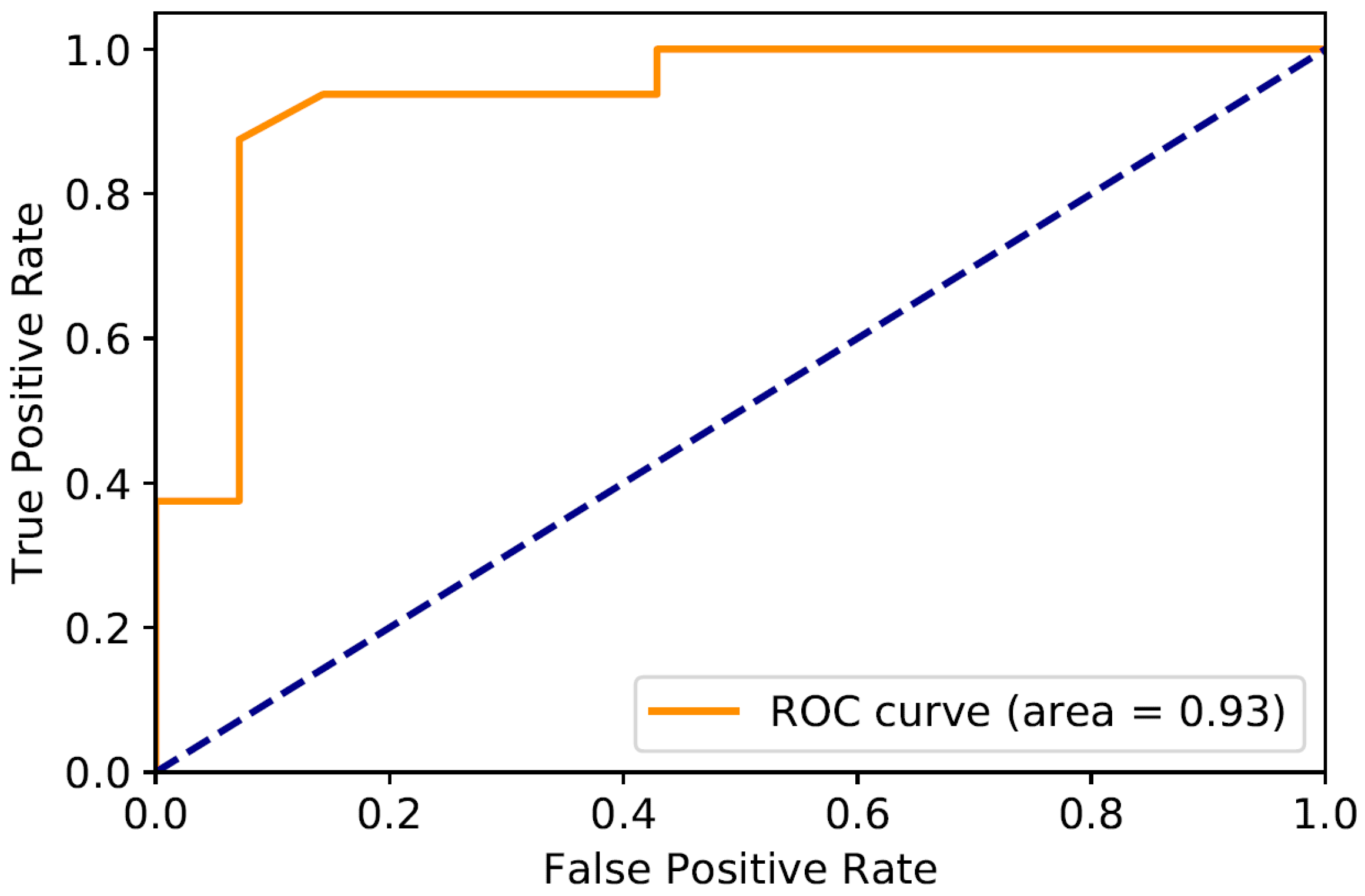
• Among the evaluated methods, random forest (RF) consistently outperformed the others, achieving the highest scores across all the evaluation metrics.
• The RF model effectively predicted oil slick occurrence using metoceanographic variables and spectrophotometric TOG measurements, producing a highly satisfactory confusion matrix and a strong area under the ROC curve (AUC), indicating reliable classification performance.
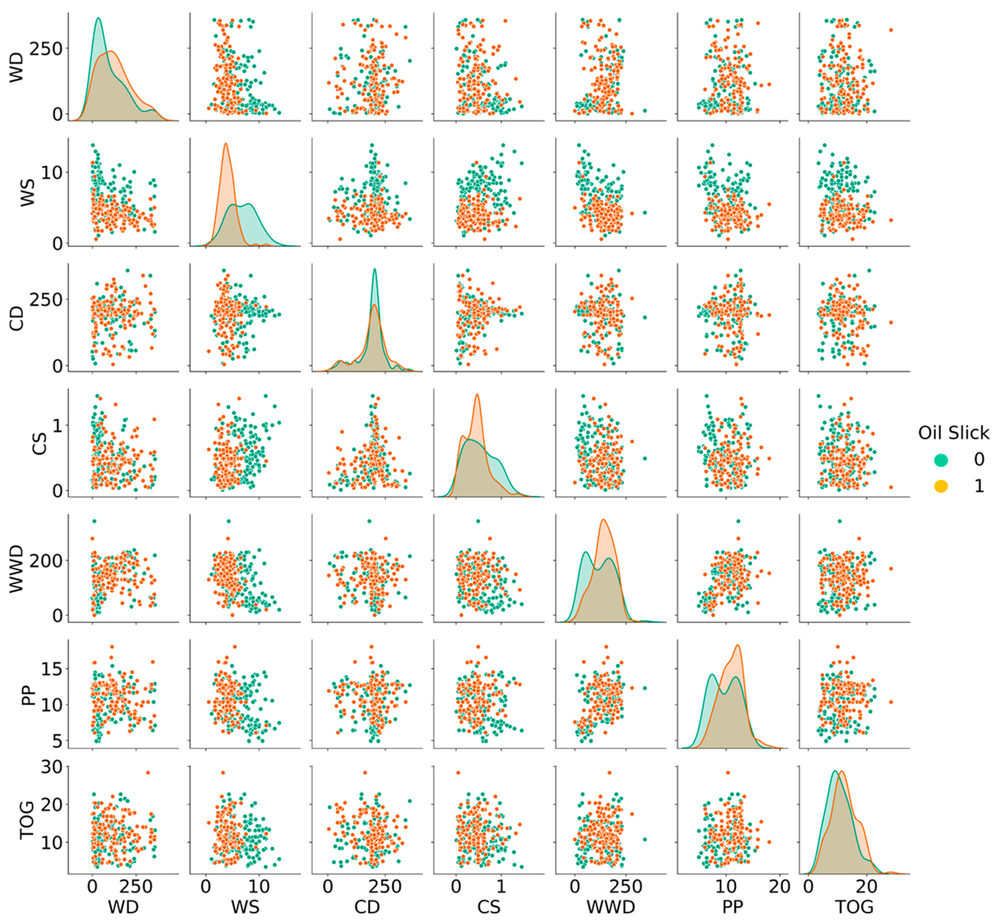
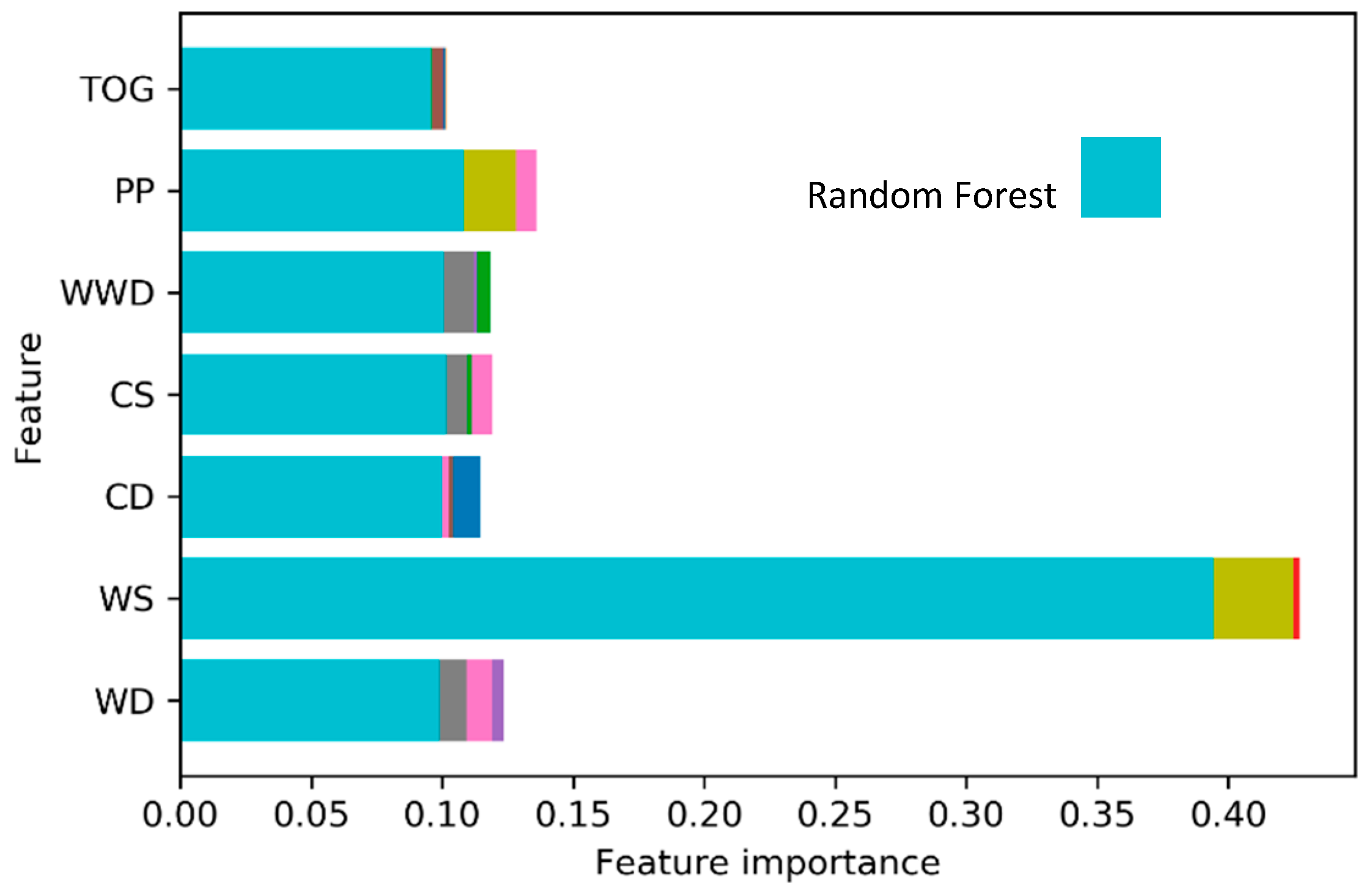
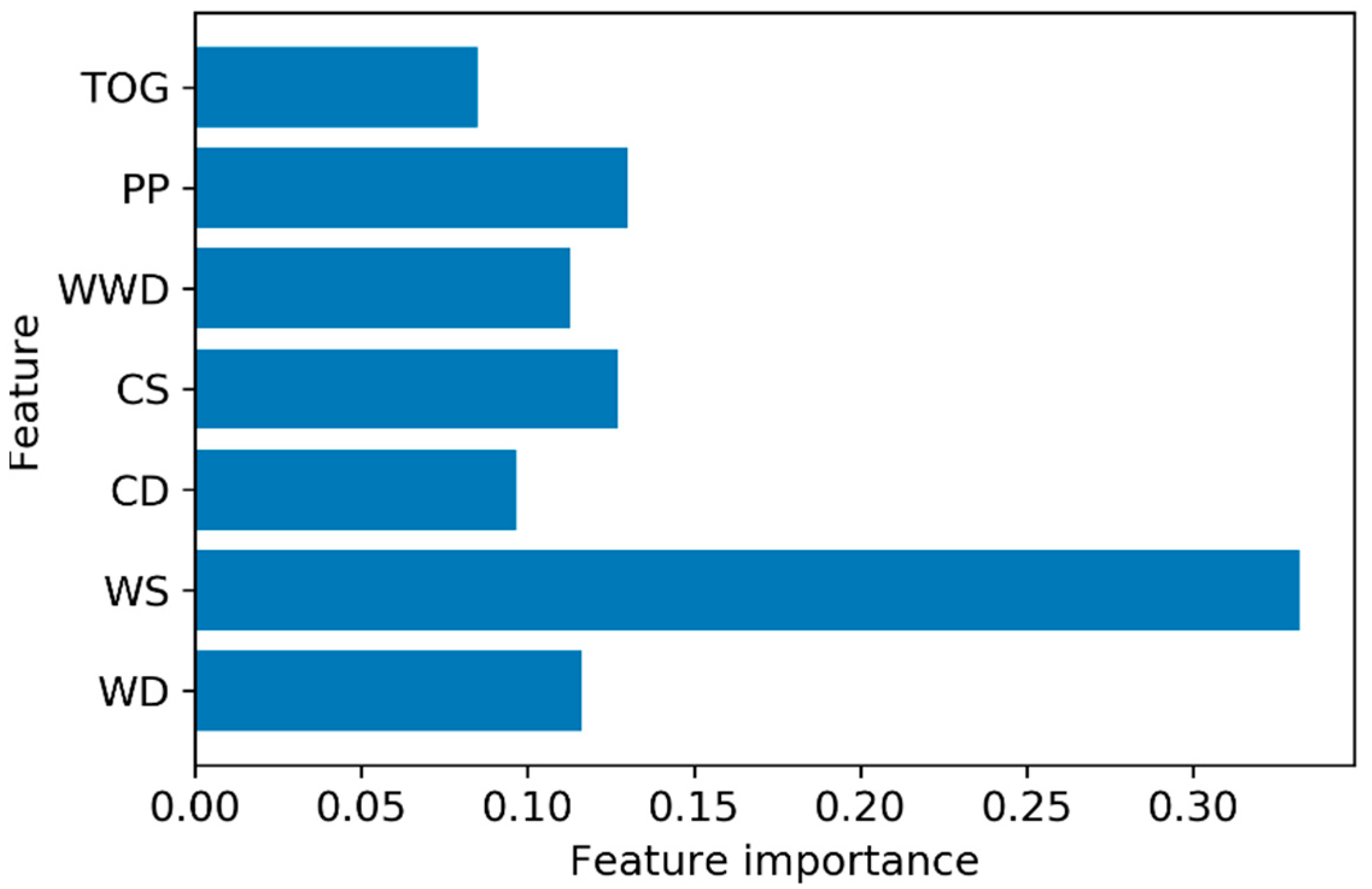
• The variable importance analysis identified WS as the most influential factor for class separation.
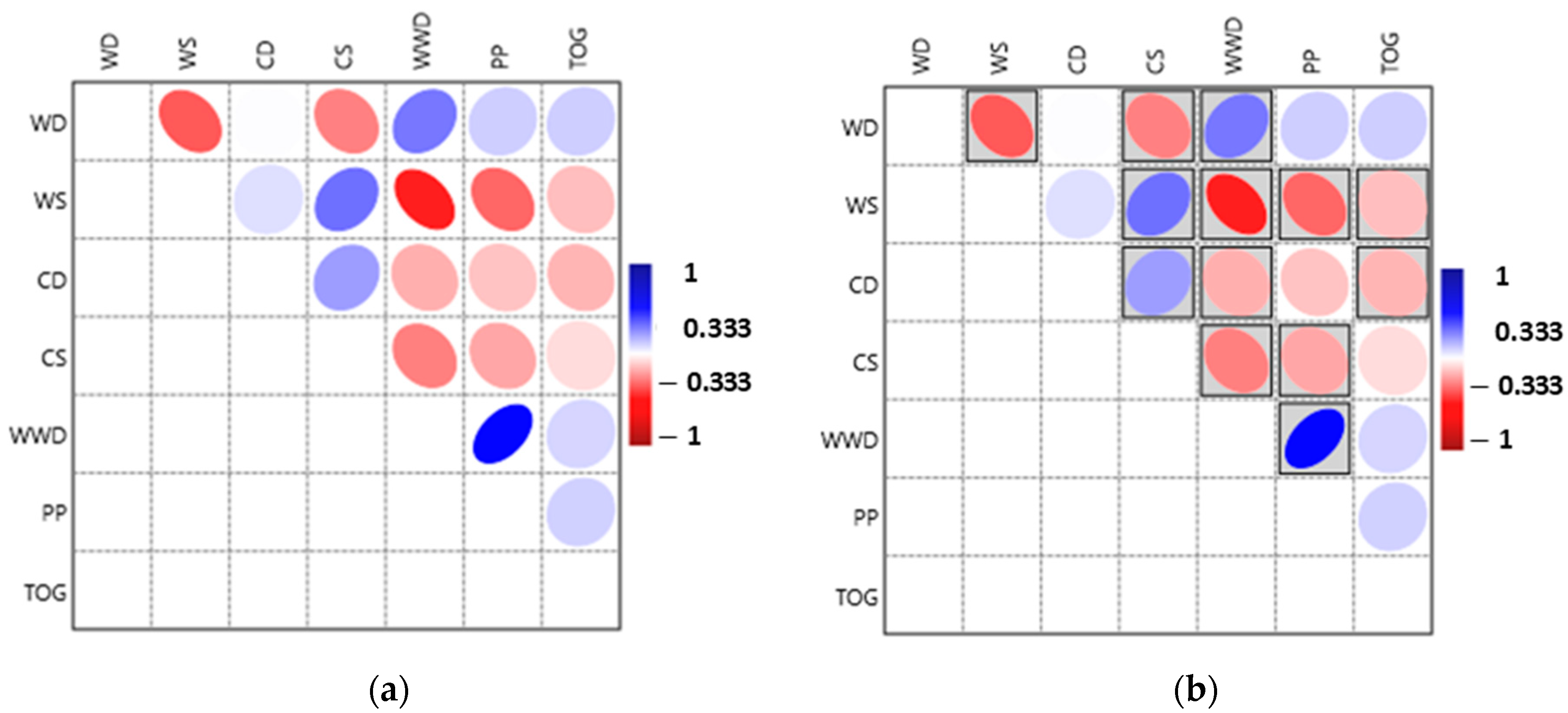
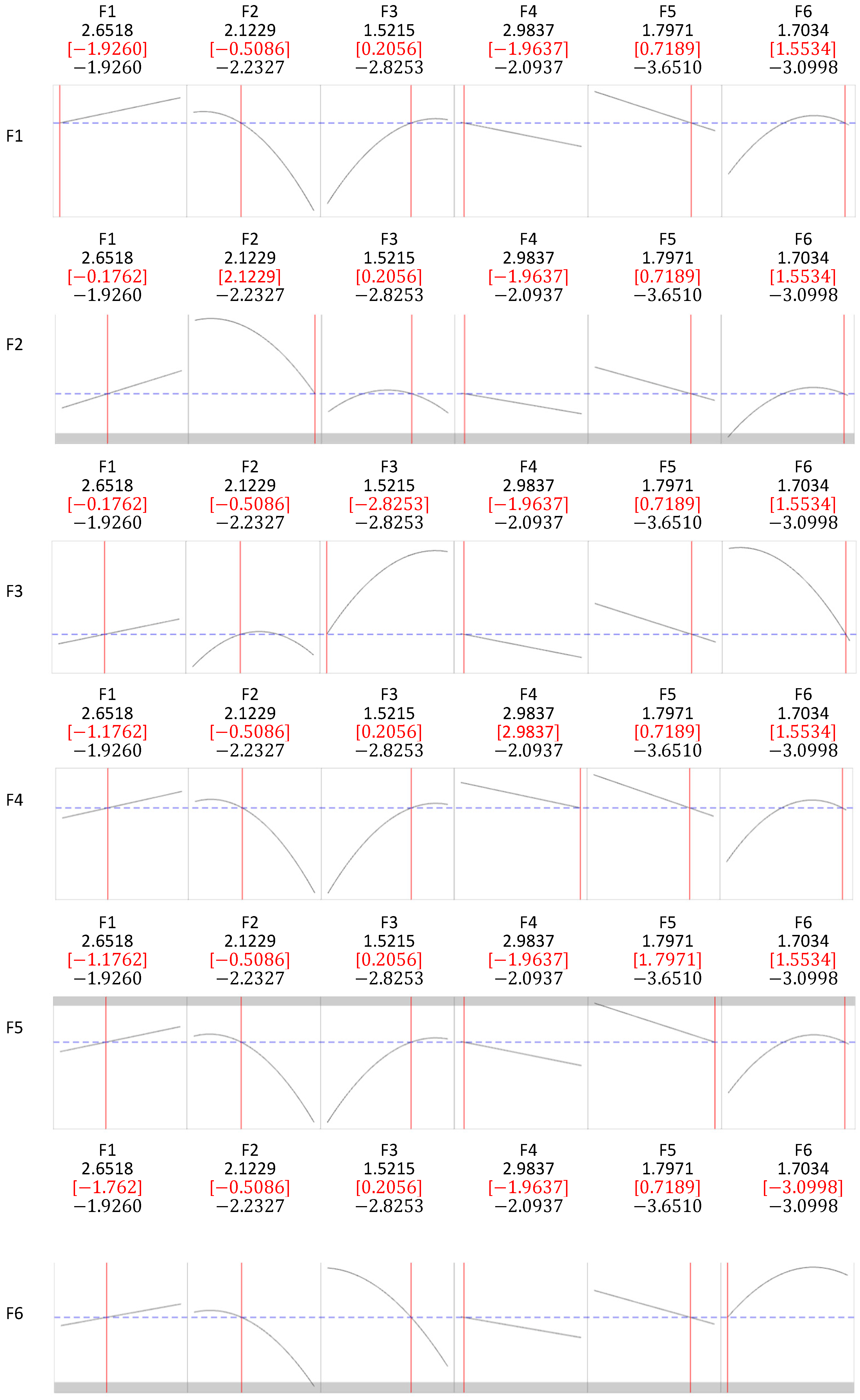
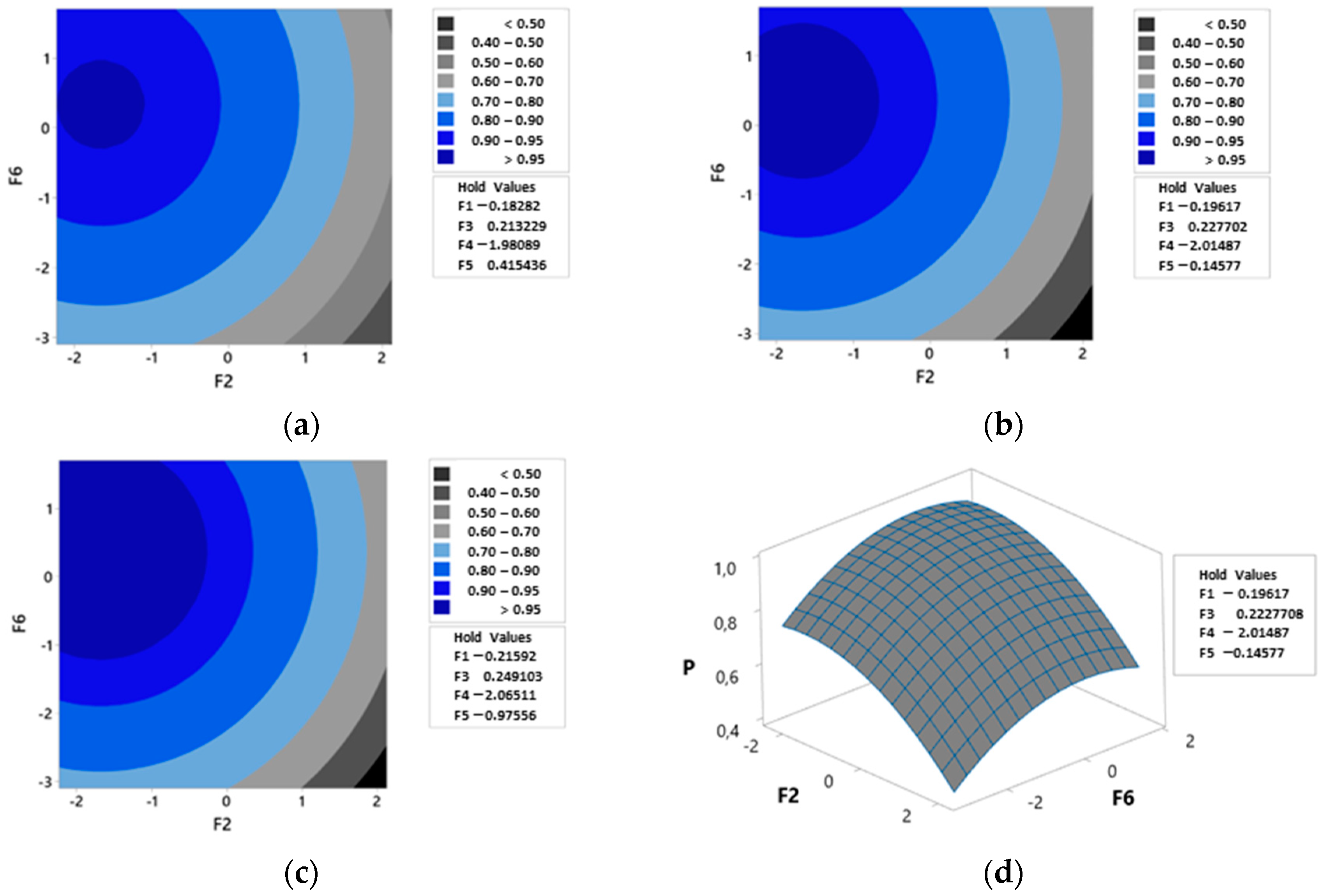
• Moderate but statistically significant correlations among predictor variables led to factor analysis, improving the model by reducing redundancy. The rotated factor scores were then converted into a central composite design (CCD) array, where the probabilities of oil slick occurrence and detection served as response variables. Optimization using the desirability technique facilitated a sensitivity analysis of the variables.
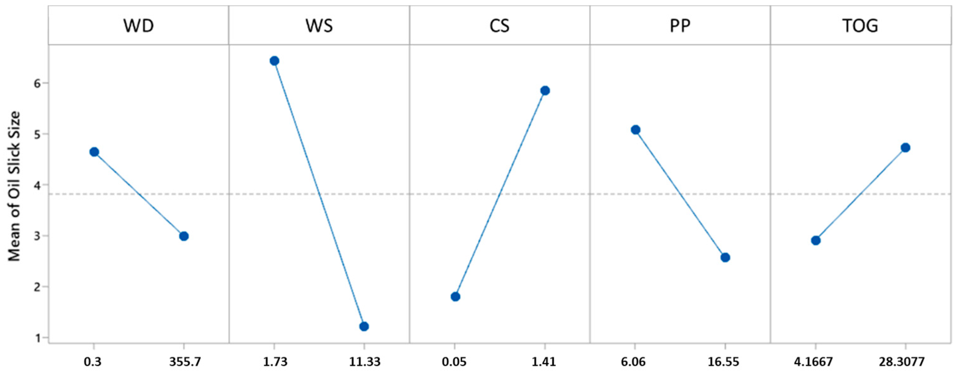
• Higher WS, WD, and CS values were associated with a lower probability of oil slick occurrence and detection.
• Conversely, higher TOG, PP, WWD, and CD values increased the probability of oil slick occurrence and detection.
• In the oil slick extension model, WS had the strongest negative effect, meaning higher wind speeds significantly reduced oil slick extension.
• CS had the strongest positive effect, meaning faster currents caused larger slicks.
• All the predictor variables were statistically significant, confirming that each variable meaningfully influenced oil slick extension.
• Higher WD, WS, and PP values were associated with smaller oil slicks, while increases in CS and TOG led to larger slicks.
• No severe multicollinearity issues were found in the model (VIF < 5), indicating model stability.

These findings provide valuable insights into how environmental and operational factors influence oil spill dynamics, supporting informed decision-making in offshore oil platform management. As a practical outcome, a user-friendly software tool was developed to assist offshore platform operators in preventing oil slick formation. One of its key features includes a visual interface displaying the probability of oil slick occurrence based on metoceanographic variables and TOG values (Figure 10).

For future research, the authors suggest an experimental study to better establish the cause-and-effect relationship between the variables and oil slick occurrence and extension. The predictor developed in this study, based on nearly three years of observational data from an offshore oil platform, proved useful for forecasting oil slicks. However, observational studies have limited power in uncovering deeper causal relationships compared to experimental approaches. The observational method was used here due to the inherent challenges of conducting experiments with meteoceanographic variables and TOG metrics.

References

1. Klemz, A.C.; Damas, M.S.P.; Weschenfelder, S.E.; González, S.Y.G.; Pereira, L.d.S.; Costa, B.R.d.S.; Junior, A.E.O.; Mazur, L.P.; Marinho, B.A.; de Oliveira, D.; et al. Treatment of real oilfield produced water by liquid-liquid extraction and efficient phase separation in a mixer-settler based on phase inversion. Chem. Eng. J. 2021, 417, 127926. [Google Scholar] [CrossRef]
2. CONAMA Resolution No. 393/2007. Available online: http://www.braziliannr.com/brazilian-envi%0Aronmentallegislation/conama-resolution-39307/ (accessed on 4 May 2021).
3. National Oceanic and Atmospheric Administration (NOAA). Open Water Oil Identification Job Aid (NO-AA-CODE) for Aerial Observation; NOAA/ORCA: Silver Spring, MD, USA, 2016.
4. Office of Response and Restoration. Trajectory Analysis Handbook; National Oceanic and Atmospheric Administration (NOAA): Silver Spring, MD, USA, 2012. Available online: https://response.restoration.noaa.gov/sites/default/files/Trajectory_Analysis_Handbook.pdf (accessed on 23 April 2021).
5. Röhrs, J.; Dagestad, K.F.; Asbjørnsen, H.; Nordam, T.; Skancke, J.; Jones, C.E.; Brekke, C. The effect of vertical mixing on the horizontal drift of oil spills. Ocean Sci. 2018, 14, 1581–1601. [Google Scholar] [CrossRef]
6. Zhang, Y.; Guo, W.; Liang, D.; Wu, W.; Zhao, Y.; Wu, L. Effect of Wind-Wave-Current Interaction on Oil Spill in the Yangtze Estuary. J. Mar. Sci. Eng. 2023, 11, 494. [Google Scholar] [CrossRef]
7. Elliott, A.J.; Hurford, N. The effects of wind and turbulence on the spreading of oil slicks. N. Z. J. Mar. Freshw. Res. 1977, 11, 311–321. [Google Scholar] [CrossRef]
8. Drozdowski, A.; Nudds, S.; Hannah, C.G.; Niu, H.; Peterson, I. Modeling oil spill transport and fate in the Arctic: A review. Arct. Sci. 2018, 4, 314–339. [Google Scholar] [CrossRef]
9. Hoult, D.P. Oil spreading on the sea. Annu. Rev. Fluid Mech. 1979, 4, 341–368. [Google Scholar] [CrossRef]
10. Reed, M.; Turner, C.; Odulo, A. Oil spill modeling: Risk analysis and response strategies. In Oil Spill Science and Technology, 2nd ed.; Spaulding, M.L., Ed.; Elsevier: Amsterdam, The Netherlands, 2018; pp. 163–220. [Google Scholar] [CrossRef]
11. Ren, L.; Wang, Y.; Zhang, W.; Yang, H.; Wang, H.; Wei, J.; Flores Mateos, L.M. Characterizing wind fields at multiple temporal scales: A case study of the adjacent sea area of Guangdong–Hong Kong–Macao Greater Bay Area. Energy Rep. 2022, 8, 212–223. [Google Scholar] [CrossRef]
12. Albergel, C.; Polcher, J.; Mahendran, A.; Prigent, C. Impact of wind and precipitation on oil slick drift. Ocean Sci. 2019, 15, 725–741. [Google Scholar] [CrossRef]
13. Larasati, A.; Husrin, S.; Pranowo, W.S. Spatial and temporal oil spill distribution analysis using remote sensing data in the Makassar Strait. AIP Conf. Proc. 2023, 3069, 020133. [Google Scholar] [CrossRef]
14. Le Hénaff, M.; Kourafalou, V.H.; Srinivasan, A.; Beron-Vera, F.J.; Reniers AJ, H.M.; Shay, L.K. Surface transport pathways connecting the Deepwater Horizon oil spill regions to the Florida Keys and Southeast Florida. J. Phys. Oceanogr. 2014, 44, 145–164. [Google Scholar] [CrossRef]
15. Pisano, A.; De Dominicis, M.; Biamino, W.; Bignami, F.; Gherardi, S.; Colao, F.; Coppini, G.; Marullo, S.; Sprovieri, M.; Trivero, P.; et al. An oceanographic survey for oil spill monitoring and model forecasting validation using remote sensing and in situ data in the Mediterranean Sea. Deep. Sea Res. Part II Top. Stud. Oceanogr. 2016, 133, 132–145. [Google Scholar] [CrossRef]
16. Zatsepa, S.N.; Ivchenko, A.A.; Korotenko, K.A.; Solbakov, V.V.; Stanovoy, V.V. The Role of Wind Waves in Oil Spill Natural Dispersion in the Sea. Oceanology 2018, 58, 517–524. [Google Scholar] [CrossRef]
17. Daneshgar Asl, S.; Dukhovskoy, D.S.; Bourassa, M.; MacDonald, I.R. Hindcast modeling of oil slick persistence from natural seeps. Remote Sens. Environ. 2017, 189, 96–107. [Google Scholar] [CrossRef]
18. Xu, J.; Cheng, M.; Li, B.; Chu, L.; Dong, H.; Yang, Y.; Qian, S.; Huang, Y.; Yuan, J. Oil Slick Identification in Marine Radar Image Using HOG, Random Forest and PSO. IEEE Geosci. Remote Sens. Lett. 2024, 21, 1–5. [Google Scholar] [CrossRef]
19. Ebecken, N.F.F.; de Miranda, F.P.; Landau, L.; Beisl, C.; Silva, P.M.; Cunha, G.; Lopes, M.C.S.; Dias, L.M.; Carvalho, G.d.A. Computational Oil-Slick Hub for Offshore Petroleum Studies. J. Mar. Sci. Eng. 2023, 11, 1497. [Google Scholar] [CrossRef]
20. Genovez, P.C.; Ponte, F.F.d.A.; Matias, Í.d.O.; Torres, S.B.; Beisl, C.H.; Mano, M.F.; Silva, G.M.A.; Miranda, F.P.d. Development and Application of Predictive Models to Distinguish Seepage Slicks from Oil Spills on Sea Surfaces Employing SAR Sensors and Artificial Intelligence: Geometric Patterns Recognition Under a Transfer Learning Approach. Remote Sens. 2023, 15, 1496. [Google Scholar] [CrossRef]
21. Wang, L.; Lu, Y.; Wang, M.; Zhao, W.; Lv, H.; Song, S.; Wang, Y.; Chen, Y.; Zhan, W.; Ju, W. Mapping of oil spills in China Seas using optical satellite data and deep learning. J. Hazard. Mater. 2024, 480, 135809. [Google Scholar] [CrossRef] [PubMed]
22. Breiman, L. Random Forests. Mach. Learn. 2001, 45, 5–32. [Google Scholar]
23. Musbah, H.; Aly, H.H.; Little, T.A. Energy management of hybrid energy system sources based on machine learning classification algorithms. Electr. Power Syst. Res. 2021, 199, 107436. [Google Scholar] [CrossRef]
24. Dai, B.; Gu, C.; Zhao, E.; Qin, X. Statistical model optimized random forest regression model for concrete dam deformation monitoring. Struct. Control Health Monit. 2018, 25, 1–15. [Google Scholar] [CrossRef]
25. Sanquetta, C.R.; Piva, L.R.; Wojciechowski, J.; Corte, A.P.; Schikowski, A.B. Volume estimation of Cryptomeria japonica logs in southern Brazil using artificial intelligence models. South. For. J. For. Sci. 2018, 80, 29–36. [Google Scholar] [CrossRef]
26. Zuo, W.; Zhang, D.; Wang, K. On kernel difference-weighted k-nearest neighbor classification. Pattern Anal. Appl. 2008, 11, 247–257. [Google Scholar] [CrossRef]
27. Zhang, S.; Cheng, D.; Deng, Z.; Zong, M.; Deng, X. A novel kNN algorithm with data-driven k parameter computation. Pattern Recognit. Lett. 2018, 109, 44–54. [Google Scholar] [CrossRef]
28. Ezzat, A.; Elnaghi, B.E.; Abdelsalam, A.A. Microgrids islanding detection using Fourier transform and machine learning algorithm. Electr. Power Syst. Res. 2021, 196, 107224. [Google Scholar] [CrossRef]
29. El-Dahshan, E.S.A.; Bassiouni, M.M. Computational intelligence techniques for human brain MRI classification. Int. J. Imaging Syst. Technol. 2018, 28, 132–148. [Google Scholar] [CrossRef]
30. Zhang, S. Nearest neighbor selection for iteratively kNN imputation. J. Syst. Softw. 2012, 85, 2541–2552. [Google Scholar] [CrossRef]
31. Swetapadma, A.; Mishra, P.; Yadav, A.; Abdelaziz, A.Y. A non-unit protection scheme for double circuit series capacitor compensated transmission lines. Electr. Power Syst. Res. 2017, 148, 311–325. [Google Scholar] [CrossRef]
32. Ganbold, G.; Chasia, S. Comparison Between Possibilistic c-Means (PCM) and Artificial Neural Network (ANN) Classification Algorithms in Land Use/Land Cover Classification. Int. J. Knowl. Content Dev. Technol. 2017, 7, 57–78. [Google Scholar]
33. Islam, M.S.; Hannan, M.A.; Basri, H.; Hussain, A.; Arebey, M. Solid waste bin detection and classification using Dynamic Time Warping and MLP classifier. Waste Manag. 2014, 34, 281–290. [Google Scholar] [CrossRef]
34. Olson, J.; Valova, I.; Michel, H. WSCISOM: Wireless sensor data cluster identification through a hybrid SOM/MLP/RBF architecture. Prog. Artif. Intell. 2016, 5, 233–250. [Google Scholar] [CrossRef]
35. Puggina Bianchesi, N.M.; Romao, E.L.; Lopes, M.F.B.P.; Balestrassi, P.P.; De Paiva, A.P. A design of experiments comparative study on clustering methods. IEEE Access 2019, 7, 2953528. [Google Scholar] [CrossRef]
36. Yilmaz, I.; Kaynar, O. Multiple regression, ANN (RBF, MLP) and ANFIS models for prediction of swell potential of clayey soils. Expert. Syst. Appl. 2011, 38, 5958–5966. [Google Scholar] [CrossRef]
37. Kuo, H.F.; Faricha, A. Artificial Neural Network for Diffraction Based Overlay Measurement. IEEE Access 2016, 4, 7479–7486. [Google Scholar] [CrossRef]
38. Balestrassi, P.P.; Popova, E.; Paiva, A.P.; Marangon Lima, J.W. Design of experiments on neural network’s training for nonlinear time series forecasting. Neurocomputing 2009, 72, 1160–1178. [Google Scholar] [CrossRef]
39. Aizenberg, I.; Sheremetov, L.; Villa-Vargas, L.; Martinez-Muñoz, J. Multilayer Neural Network with Multi-Valued Neurons in time series forecasting of oil production. Neurocomputing 2016, 175, 980–989. [Google Scholar] [CrossRef]
40. Silva, I.N.; Spatti, D.H.; Flauzino, R.A.; Liboni, L.; Alves, S.F.D.R. Artificial Neural Networks: A Practical Course; Springer International Publishing AG: Cham, Switzerland, 2017. [Google Scholar]
41. Lin, S.K.; Hsiu, H.; Chen, H.S.; Yang, C.J. Classification of patients with Alzheimer’s disease using the arterial pulse spectrum and a multilayer-perceptron analysis. Sci. Rep. 2017, 11, 8882. [Google Scholar] [CrossRef]
42. Peres, A.M.; Baptista, P.; Malheiro, R.; Dias, L.G.; Bento, A.; Pereira, J.A. Chemometric classification of several olive cultivars from Trás-os-Montes region (northeast of Portugal) using artificial neural networks. Chemom. Intell. Lab. Syst. 2011, 105, 65–73. [Google Scholar] [CrossRef]
43. Wang, H.; Moayedi, H.; Kok Foong, L. Genetic algorithm hybridized with multilayer perceptron to have an economical slope stability design. Eng. Comput. 2020, 37, 3067–3078. [Google Scholar] [CrossRef]
44. Chau, N.L.; Tran, N.T.; Dao, T.P. A hybrid approach of density-based topology, multilayer perceptron, and water cycle-moth flame algorithm for multi-stage optimal design of a flexure mechanism. Eng. Comput. 2021, 38 (Suppl. S4), 2833–2865. [Google Scholar] [CrossRef]
45. Bissacot, A.C.G.; Salgado, S.A.B.; Balestrassi, P.P.; Paiva, A.; Souza, A.Z.; Wazen, R. Comparison of neural networks and logistic regression in assessing the occurrence of failures in steel structures of transmission lines. Open Electr. Electron. Eng. J. 2016, 10, 11–26. [Google Scholar] [CrossRef]
46. Hosmer, J.R.; Lemeshow, S.; Sturdvant, R.X. Applied Logistic Regression, 3rd ed.; John Wiley & Sons, Inc.: Hoboken, NJ, USA, 2013. [Google Scholar]
47. Mitiche, I.; Morison, G.; Nesbitt, A.; Hughes-Narborough, M.; Stewart, B.G.; Boreham, P. Classification of EMI discharge sources using time–frequency features and multi-class support vector machine. Electr. Power Syst. Res. 2018, 163, 261–269. [Google Scholar] [CrossRef]
48. Simões, L.D.; Costa, H.J.D.; Aires, M.N.O.; Medeiros, R.P.; Costa, F.B.; Bretas, A.S. A power transformer differential protection based on support vector machine and wavelet transform. Electr. Power Syst. Res. 2021, 197, 107297. [Google Scholar] [CrossRef]
49. Erişti, H.; Uçar, A.; Demir, Y. Wavelet-based feature extraction and selection for classification of power system disturbances using support vector machines. Electr. Power Syst. Res 2010, 80, 743–752. [Google Scholar] [CrossRef]
50. Yu, X.; Yu, Y.; Zeng, Q. Support vector machine classification of streptavidin-binding aptamers. PLoS ONE 2014, 9, e99964. [Google Scholar] [CrossRef]
51. Johnson, R.A.; Wichern, D.W. Applied Multivariate Statistical Analysis, 6th ed.; Pearson Education, Inc.: Upper Saddle River, NJ, USA, 2007. [Google Scholar]
52. Rencher, A.C.; Christensen, W.F. Methods of Multivariate Analysis, 3rd ed.; John Wiley & Sons, Inc.: Hoboken, NJ, USA, 2012. [Google Scholar]
53. Aquila, G.; Peruchi, R.S.; Rotela, P., Jr.; Rocha, L.C.S.; de Queiroz, A.R.; de Oliveira Pamplona, E. Analysis of the wind average speed in different Brazilian states using the nested GR&R measurement system. Measurement 2018, 115, 217–222. [Google Scholar] [CrossRef]
54. Aquila, G.; de Queiroz, A.R.; Balestrassi, P.P.; Rotela Junior, P.; Rocha LC, S.; Pamplona, E.O.; Nakamura, W.T. Wind energy investments facing uncertainties in the Brazilian electricity spot market: A real options approach. Sustain. Energy Technol. Assess. 2020, 42, 100876. [Google Scholar] [CrossRef]
Figure 1. Graph of observations separated by class versus input variables.
Water 17 00939 g001
Figure 2. Flowchart of the methodology proposed in this paper.
Water 17 00939 g002
Figure 3. Feature importance plot for 50 random forest models. The colors represent several classifiers of Table 1.
Water 17 00939 g003
Figure 4. Feature importance plot for random forest model.
Water 17 00939 g004
Figure 5. ROC curve for random forest model.
Water 17 00939 g005
Figure 6. (a) Correlation plot; (b) correlation plot with p-value < 0.05 boxed.
Water 17 00939 g006
Figure 7. Desirability results varying one factor at a time.
Water 17 00939 g007
Figure 8. Contour and surface plots for the occurrence and detection probability model.
Water 17 00939 g008
Figure 9. Main effects plot for the oil slick extension.
Water 17 00939 g009
Figure 10. Screenshot of the oil slick prediction tool in use.
Water 17 00939 g010