Abstract
The medium river basins (MRBs) in Nepal originate from mid-hills. These medium-range rivers are typically non-snow-fed, relying on rain and other water sources. These rivers are typically small, and the sizes of medium river basins vary between 500 and 5000 km2. These MRBs are often used for irrigation and other agricultural purposes. In this analysis, we first set up, calibrated, and validated three hydrological models (i.e., HBV, HEC HMS, and SWAT) at the Kankai River Basin (one MRB in eastern Nepal). Then, the best-performing SWAT hydrological model was forced with cutting-edge climate models (CMs) using thirteen CMIP6 models under four shared socioeconomic pathways (SSPs). We employed ten bias correction (BC) methods to capture local spatial variability in precipitation and temperature. Finally, the likely streamflow alteration during two future periods, i.e., the near-term timeframe (NF), spanning from 2031 to 2060, and the long-term timeframe (FF), covering the years 2071 to 2100, were evaluated against the historical period (baseline: 1986–2014), considering the uncertainties associated with the choice of CMs, BC methods, or/and SSPs. The study results confirm that there will not be any noticeable shifts in seasonal variations in the future. However, the magnitude is projected to alter substantially. Overall, the streamflow is estimated to upsurge during upcoming periods. We observed that less deviation is expected in April, i.e., around +5 to +7% more than the baseline period. Notably, a higher percentage increment is projected during the monsoon season (June–August). During the NF (FF) period, the flow alteration will be around +20% (+40%) under lower SSPs, whereas the flow alteration will be around +30% (+60%) under higher SSPs during high flow season. Thus, the likelihoods of flooding, inundation, and higher discharge are projected to be quite high in the coming years.
1. Introduction
Nepal’s unique geographic and climatic diversity, shaped by its altitude range from 73 to 8848.86 m above mean sea level, creates distinct ecological zones that influence biodiversity and human livelihoods [1,2]. The country is divided into three geographic regions: the Himalayas, Mountains and Hills, and the Lowland Tarai, each with its own environmental complexity [3]. Major rivers such as the Mahakali, Karnali, Narayani, and Koshi originate in the Himalayan region, where snow and glacier meltwater are predominant [4]. These rivers traverse the rugged terrains of the mountains and hills, contributing significantly to the country’s freshwater resources [5]. Nepal is endowed with substantial water resources, estimated at 210,200 million cubic meters annually, accounting for 2.3% of the world’s total renewable freshwater resources [6]. However, the hydrology of the Himalayan region is undergoing rapid changes due to climate change, exacerbating the vulnerability of the country to natural disasters such as floods, landslides, and droughts [7,8,9].
Climate change is particularly impactful in Nepal, where the hydrological regime is highly sensitive to changes in precipitation and temperature patterns [10,11]. Increasing temperatures, erratic rainfall, and more frequent extreme events are threatening water security and human well-being [12,13]. Nepal ranks 4th in terms of vulnerability to climate-related hazards and 20th among the most multi-hazard-prone countries globally, with approximately 80% of its population living in high-risk areas [14,15]. The country’s summer monsoon, occurring from June to September, contributes over 80% of its annual rainfall and is critical for agriculture, which is predominantly rain-fed [16]. These challenges highlight the need for robust water resource management strategies that account for future climate variability.
Previous studies have highlighted the impacts of climate change on hydrological processes in Nepal, focusing on snow-fed river basins and large-scale river systems [17,18,19]. However, medium-sized river basins (MRBs), which are predominantly rain-fed and used for irrigation and other agricultural purposes, have received less attention [20]. These basins, typically ranging in size from 500 to 5000 km², are highly susceptible to changes in precipitation patterns and are critical for local livelihoods [21]. For example, the Kankai River Basin, located in eastern Nepal, is a significant trans-boundary river system that supports hydropower generation and provides irrigation water to downstream areas [22]. Understanding the hydrological dynamics of such basins under changing climate conditions is essential for effective water resource management.
Hydrological models are crucial tools for simulating and predicting how river basins respond to climatic and meteorological influences. Conceptual hydrological models, such as the Hydrologiska Byråns Vattenbalansavdelning (HBV) model [23], the Hydrologic Engineering Center’s Hydrologic Modeling System (HEC-HMS) [24,25], and the Soil and Water Assessment Tool (SWAT) [26], have been widely used for this purpose. These models vary in their ability to simulate different hydrological processes and are often calibrated and validated using historical data to ensure their accuracy [27,28,29]. The HBV model is particularly effective in simulating snow and glacier melt processes in high-altitude regions [30], while SWAT is better suited for agricultural landscapes due to its ability to incorporate land use and soil characteristics [26]. HEC-HMS, on the other hand, is known for its robustness in simulating peak flows and is widely used for flood analysis [24,25].
Recent advancements in climate modeling, such as the Coupled Model Intercomparison Project Phase 6 (CMIP6) [31,32], provide improved frameworks for simulating future climate conditions. CMIP6 introduces Shared Socioeconomic Pathways (SSPs) that combine socioeconomic scenarios with Representative Concentration Pathways (RCPs), offering more comprehensive projections of future climate impacts [33]. These models, when combined with bias correction techniques, can provide reliable inputs for hydrological simulations [34]. However, no studies in Nepal have yet utilized CMIP6 outputs to project future water availability in medium-sized river basins such as the Kankai River Basin.
1.1. Objective
This manuscript investigates the impacts of climate change on streamflow in the Kankai River Basin, a medium-sized river basin in eastern Nepal. The study is motivated by the need to understand how changing climatic conditions, particularly alterations in precipitation and temperature patterns, will affect water availability and hydrological dynamics in the region. Given Nepal’s high vulnerability to climate-related hazards and its reliance on freshwater resources for agriculture, hydropower, and domestic use, this research aims to provide a comprehensive assessment of future hydrological changes using advanced modeling techniques and climate projections. The findings are expected to contribute to the development of robust water resource management strategies and climate adaptation plans in the region.
1.2. Detailed Objectives
- Model Setup and Calibration
Objective: To set up, calibrate, and validate three hydrological models (HBV, HEC-HMS, and SWAT) using historical data from the Kankai River Basin.
Significance: Accurate calibration of hydrological models is essential for reliable predictions of future streamflow. By using multiple models, we can compare their performance and identify the most suitable model for the study area.
- 2.
- Historical Streamflow Simulation
Objective: To evaluate the performance of the three hydrological models in simulating historical streamflow in the Kankai River Basin.
Significance: Assessing the models’ ability to reproduce historical hydrological conditions helps to validate their applicability for future projections. This step ensures that the models can accurately capture the temporal dynamics and volume of streamflow.
- 3.
- Future Streamflow Projections
Objective: To project future streamflow alterations under different climate scenarios using bias-corrected climate projections from 13 CMIP6 models under four Shared Socioeconomic Pathways (SSPs).
Significance: Understanding how streamflow will change in the future is crucial for planning water resource projects, such as irrigation systems, hydropower facilities, and flood control infrastructure. Projections under different SSPs provide insights into potential hydrological extremes and their implications for water availability and flood risk.
- 4.
- Uncertainty Assessment
Objective: To assess the uncertainties associated with climate model selection, bias correction methods, and socioeconomic pathways.
Significance: Climate projections are subject to uncertainties arising from model selection, bias correction techniques, and future socioeconomic scenarios. Evaluating these uncertainties helps in developing more robust and reliable water management strategies by accounting for potential variability in future hydrological conditions.
- 5.
- Contribution to Water Resource Management
Objective: To provide valuable insights for water resource management and climate adaptation strategies in the Kankai River Basin and similar regions.
Significance: The findings of this study will inform policymakers and water resource managers about the projected changes in streamflow and potential risks associated with climate change. This information is critical for designing adaptive management strategies, improving flood control infrastructure, and ensuring sustainable water use in the region.
The manuscript aims to fill the research gap in understanding the hydrological impacts of climate change in medium-sized river basins, specifically focusing on the Kankai River Basin in Nepal. By integrating multiple hydrological models with state-of-the-art climate projections, the study provides a comprehensive assessment of future streamflow alterations and their uncertainties. The results are expected to contribute to sustainable water resource management and climate adaptation efforts in the region, ultimately enhancing resilience to climate change impacts.
1.3. Research Gap
Previous studies have extensively highlighted the impacts of climate change on hydrological processes in Nepal, focusing primarily on snow-fed river basins and large-scale river systems. However, medium-sized river basins (MRBs), which are predominantly rain-fed and used for irrigation and other agricultural purposes, have received less attention. These basins, typically ranging in size from 500 to 5000 km2, are highly susceptible to changes in precipitation patterns and are critical for local livelihoods. For example, the Kankai River Basin, located in eastern Nepal, is a significant transboundary river system that supports hydropower generation and provides irrigation water to downstream areas. Understanding the hydrological dynamics of such basins under changing climate conditions is essential for effective water resource management.
2. Materials and Methods
This research assesses climate change impacts on streamflow in the Kankai River Basin using advanced hydrological models. Key models include HBV (developed by SMHI, Sweden, for continuous runoff simulation), HEC-HMS (developed by the U.S. Army Corps of Engineers for rainfall-runoff transformation), and SWAT (developed by the USDA Agricultural Research Service for watershed-scale water balance). Calibration and validation were conducted using historical data, with SWAT enhanced via ArcSWAT (ArcGIS version 10.5). Future climate conditions were simulated using CMIP6 projections under various SSPs, with bias correction applied to refine accuracy. This integrated approach provides a comprehensive framework for evaluating hydrological changes and uncertainties. The research was carried out to analyze the impact of future climate change on river flow at the medium-sized watershed basin of Nepal. A framework of the overall methodology is presented in Figure 1.

Figure 1.
The framework of the overall method.
2.1. Regional Characteristics
2.1.1. Study Area
The Kankai River is a significant transboundary river that flows through the hills of Ilam and the plains of Jhapa District in Nepal. It begins at the confluence of the Mai Khola and Deb Mai Khola rivers, with a drainage area of approximately 1148 km2. The river flows southward into India, where it joins the Mahananda River in Bihar. Covering a total area of about 1294 km2, approximately 40% of the basin lies below 600 m, while only 12% is situated above 2000 m. The altitude within the basin ranges from 73 m in the southern region to 3603 m in the north [26], as presented in Figure 2.
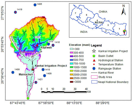
Figure 2.
Site of stream grid and meteorological stations. Note: 1–7 represent the seven provinces of Nepal.
The Kankai River Basin is wider at the headwater and narrows downstream. It is a transboundary river that begins from the central mountain and inclines towards the lowland region of Tarai. Mai Khola and Puwa Khola are the main tributaries of the Kankai River. The river basin is a rain-fed, perennial system, with its water resources highly susceptible to climatic variability. Given its critical role in supporting hydropower generation and providing irrigation water to the downstream southern plains, a comprehensive understanding of its hydrologic dynamics is essential for effective water resource management.
2.1.2. Hydrometeorological Characteristics
Nepal’s hydrometeorological characteristics are influenced by its diverse topography, ranging from the lowland Terai plains to the snow-capped peaks of the Himalayas. The country has a monsoon-dominated climate, with four main seasons: winter, spring, monsoon, and autumn. During the monsoon season (June to September), the southwest monsoon brings heavy rainfall, especially to the Terai region, while the mountainous areas receive less precipitation. Nepal’s rivers, such as Koshi, Gandaki, and Karnali, are primarily fed by snowmelt and rainfall, providing vital water resources for agriculture, domestic use, and hydroelectric power generation. However, these rivers are also prone to flooding and landslides during the monsoon season, causing damage to infrastructure and livelihoods. Additionally, some areas, particularly in the rain shadow of the Himalayas, experience droughts and water scarcity during dry months. These extreme weather events and seasonal water fluctuations pose challenges for managing Nepal’s water resources, agriculture, and disaster preparedness. Figure 3 illustrates the temporal variation in everyday rainfall and daily highest and lowest temperatures in the study area. Basin-wide average precipitation was calculated by averaging the data from nine precipitation stations. Similarly, average maximum and minimum temperatures were derived by averaging the values recorded at climate stations. These individual rainfall and temperature data points were utilized as inputs for driving the hydrological model. Similarly, Figure 4 reveals the temporal variation in daily river discharge at the Mainachuli station.
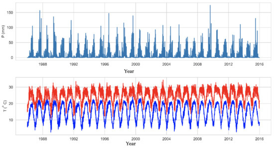
Figure 3.
Temporal variations in daily weather. Note: Precipitation (P), maximum temperature (red), and minimum temperature (blue).
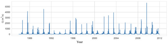
Figure 4.
Temporal variation of daily river discharge at Mainachuli.
2.1.3. Data Acquisition and Processing
The essential data for this research contained the DEM, river network, land cover data, soil data, and climate data time series. These datasets were sourced from various references, as shown in Table 1. The input data were pre-processed and restructured to align with the model’s requirements.

Table 1.
Data point type and description.
2.1.4. Hydrometeorological Data
This study collected daily precipitation and temperature data from meteorological and hydrological station maintained by the Department of Hydrology and Meteorology of the Government of Nepal. Daily rainfall accounts from nine rainfall stations and daily lowest and highest temperature data from four climate stations were utilized to configure the hydrological model. The particulars of the hydrometeorological stations in the research area are outlined in Table 2.
Table 2.
List of hydrometeorological stations.
Daily hydrological data spanning the years 2005 to 2011 at the Mainachuli hydrological station were used for hydrological model standardization and validation because of the good data quality of the discharge data during that period. The hydrological station is also located near the intake of the Kankai Irrigation Project. Daily discharge data are the most granular data publicly accessible from the DHM.
2.1.5. Land Use Land Cover and Soil Data
The research gathered land user land cover data from the International Centre for Integrated Mountain Development. The LULC map for the year 2010 used in this study was created by ICIMOD (2013) at a spatial resolution of 30 m. Further details on the LULC data can be found in ref. [29]. Over half of the study area is occupied by forest, and approximately 36% is used for agriculture (Figure 5). Shrub and grasslands cover about 5% of the study area. The remaining 2.5% is covered by water (1.5%), barren land (0.5%), and urban (0.5%). The resolution of the land surface map influences the accuracy of water balance and sediment yield predictions for a basin. In addition, the number of HRUs generated also depends on the resolution. Higher-resolution soil data increase model prediction accuracy [30].

Figure 5.
Spatial distribution of land use pattern and soil types of the Kankai River Basin.
This study utilized the Soil and Terrain Database (SOTER) for Nepal, which was developed by the International Soil Resource and Information Center (ISRIC). The SOTER soil data has a spatial resolution of 1:1,000,000. The study basin consists of seven soil types. Over half of the study area is occupied by chromic cambisols (CMx), with sand, silt, and clay percentages of roughly 40, 21, and 39, respectively (Figure 5). Other dominant soil types are dystric regosols (RGd), with 15% coverage of the study area, and the soil type has sand, silt, and clay percentages of roughly 82, 7, and 11%, respectively, and eutric cambisols (CMe), with 10% coverage of the study area, and the soil type has sand, silt, and clay percentages of roughly 36, 37, and 27%, respectively. Other soil types have 2 to 3% coverage. Overall, upstream sub-basins have camisole-dominant soil types. The twenty-six sub-basins used in this study have sub-basin areas varying from less than 0.5 km2 to 108 km2.
2.1.6. Climate Model Data
The climate models used to analyze future streamflow are summarized in Table 3. This study used the historical period (1986–2014) as a baseline and evaluated two future periods: the near-term timeframe (2031–2060) and the long-term timeframe (2071–2100). Four scenarios were selected for analysis: (i) SSP 1 combined with RCP 2.6 (referred to as SSP 126), (ii) SSP 2 combined with RCP 4.5 (SSP 245), (iii) SSP 3 combined with RCP 7.0 (SSP 370), and (iv) SSP 5 combined with RCP 8.5 (SSP 585). The selected CMIP6 models incorporated earlier RCP information while offering more detailed and realistic future projection pathways [32,33]. Additionally, the combined climate scenarios enhanced the understanding of potential future conditions. Assessing water availability under current and projected climatic conditions is essential for planning and managing water infrastructure, including irrigation systems, water supply networks, and hydropower facilities.
Table 3.
Climate models used in the research.
2.2. DEM in Hydrological Modeling
In this study, the ALOS PALSAR 12.5 m Digital Elevation Model (DEM) played a crucial role in defining the topographical and hydrological characteristics of the Kankai River Basin, which was essential for setting up and running the hydrological models (HBV, HEC-HMS, and SWAT). The DEM was processed and analyzed to support various hydrological modeling components, ensuring accurate representation of watershed characteristics.
2.2.1. Watershed Delineation and Stream Network Extraction
The DEM was used to delineate watershed boundaries, identify drainage networks, and define sub-basins. Using GIS-based hydrological tools, flow direction and accumulation were determined to map the main river course and its tributaries. The stream network was extracted by applying a flow accumulation threshold, distinguishing between major and minor streams. This process ensured accurate hydrological connectivity within the basin, allowing for refined water flow analysis.
2.2.2. Elevation Bands for HBV Model
For the HBV model, the DEM was utilized to divide the basin into 10 elevation bands at 750 m intervals. These elevation bands were crucial for representing precipitation distribution, temperature lapse rates, and runoff generation at different altitudes. The inclusion of elevation-based classification improved the model’s ability to simulate hydrological processes under diverse terrain conditions.
2.2.3. Slope Classification and HRU Definition for SWAT Model
The DEM was instrumental in classifying slopes into four categories: 0–15%, 15–45%, 45–60%, and >60%. These classifications were used to define Hydrologic Response Units (HRUs) by integrating land use, soil type, and slope characteristics. The HRUs played a significant role in determining runoff generation, infiltration, and soil erosion processes, thereby enhancing the accuracy of hydrological simulations in the SWAT model.
2.2.4. Channel and Sub-Basin Parameterization for HEC-HMS Model
The DEM provided essential elevation and slope data for the HEC-HMS model, aiding in computing channel properties and routing parameters. It helped to estimate time of concentration and surface roughness, both of which influence flood hydrograph generation and overall water flow dynamics within the basin.
2.2.5. Impact of DEM Resolution on Model Accuracy
The selection of a high-resolution DEM (12.5 m) was critical for improving hydrological model accuracy. Coarser-resolution DEMs often oversimplify watershed topography, leading to inaccuracies in streamflow simulation. The fine resolution allowed for a more detailed representation of terrain variability, resulting in improved calibration and performance of the hydrological models.
By integrating the DEM-derived topographic data into hydrological modeling, we enhanced the reliability of streamflow simulations and water resource assessments. This comprehensive approach enabled better predictions of hydrological responses under climate change scenarios, supporting effective water resource management and flood risk mitigation.
2.3. Overview of CMIP6
See Supplemental Material at S4 for more about the model. To adapt global climate change scenarios to a local scale suitable for basin-level analysis, a downscaling method is required. The dynamic downscaling technique enhances resolution by utilizing a Regional Climate Model (RCM) that incorporates boundary conditions derived from Global Climate Model (GCM) simulations [35]. A new series of coordinated climate experiments was recently conducted as part of phase 6 of the CMIP initiative CMIP5 projections, relying on 2100 radiative forcing values corresponding to four greenhouse gas (GHG) concentration pathways. Conversely, CMIP6 incorporates Shared Socioeconomic Pathways (SSPs) while building upon the foundational premises of CMIP5 scenarios. Figure 6 presents an overview of CMIP6 compared with CMIP5 scenarios. The selected scenarios in the current study are SSP 126, SSP 245, SSP 370, and SSP 585.

Figure 6.
Overview of CMIP6. Note: CMIP6 compared with CMIP5 scenarios. The selected scenarios in the analysis are SSP 126, SSP 245, SSP 370, and SSP 585.
SSP 585 represents the scenario with the highest fossil-fuel development and corresponds to RCP 8.5, representing a high-radiative imposing pathway that projects an increase to 8.5 W/m2 by the end of the century. On the other hand, SSP 245 reflects a middle-ground scenario regarding socioeconomic challenges for mitigation and adaptation. It aligns with RCP 4.5, which represents a steadiness pathway without overrun, stabilizing at 4.5 W/m2 after 2100. SSP 126 represents sustainability regarding socioeconomic challenges for mitigation and adaptation. It corresponds to the lower emission scenario of RCP 2.6, i.e., peak in radiating forcing at ~3 W/m2 before the end of the century and falling off to 2.6 W/m2 by 2100. Finally, SSP 370 represents the highest socioeconomic challenges for mitigation and adaptation and corresponds to emission scenarios between RCP 4.5 and RCP 8.5. A sample plot of the temporal variations in projected precipitation and temperature (Tmax and Tmin) under thirteen CMIP6 climate models at a climate station at the Illam Tea Estate is presented in Figure 7.
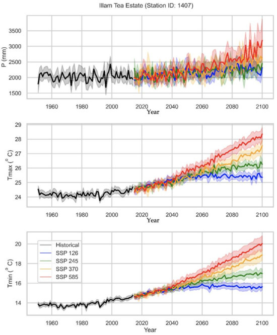
Figure 7.
Plot of historical and future projections of weather at a sample station.
In CMIP6 climate model simulations, the projection scenarios are generated from 2015 onward (i.e., prospective run), and the period up to 2014 is simulated as a historic run (i.e., retrospective run). That means the historical simulation for any climate model is available up to 2014, and SSP scenarios are available from 2015. In this study, the baseline stage from the historical data spanned from 1986 to 2014. The performance of climate model outputs for precipitation and temperature was therefore compared with observations during the same period. For projected future scenarios, this study focused on two periods: the near-term timeframe (2031–2060) and long-term timeframe (2071–2100). First, the adjusted hydrological model was used to simulate future streamflow for two future periods based on bias-corrected precipitation and temperature input at individual precipitation and climate stations. Then, the likely shifts in the future hydrological regime were compared with the baseline period hydrological regime based on the hydrological simulations. Before that, this research reports the climate model outputs in subsequent sections.
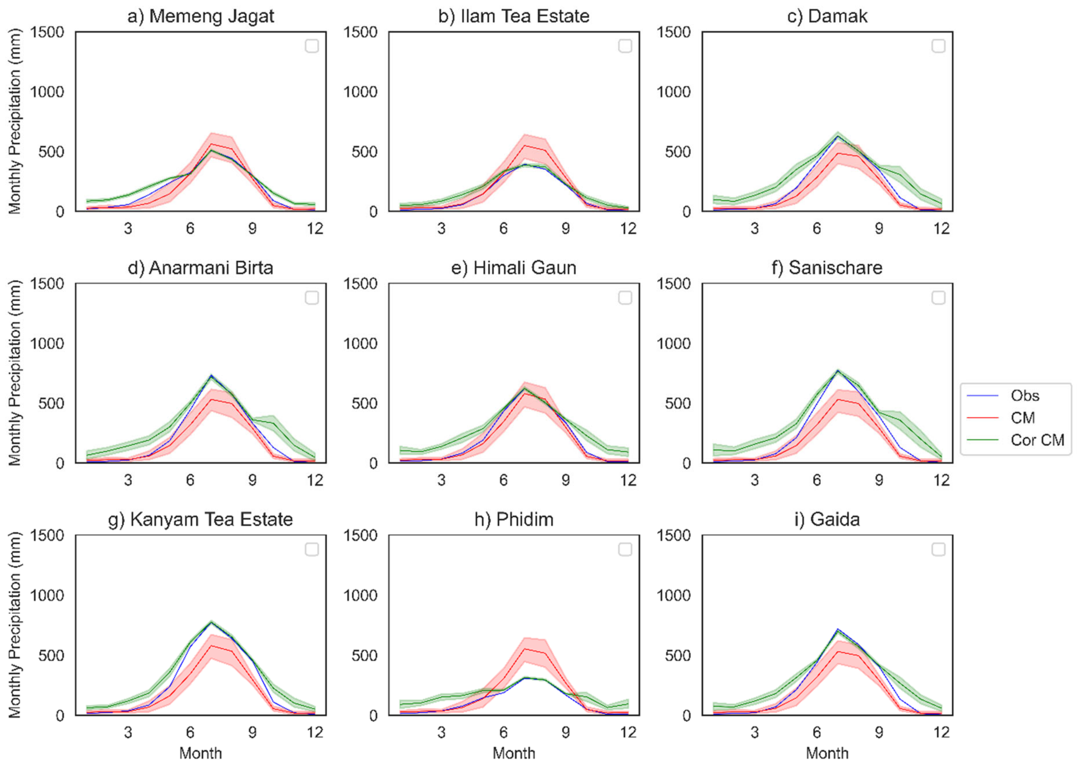
The intermodal variation of the mean monthly precipitation distribution at nine stations was based on raw and bias-corrected climate models using the power transformation method. Here, the mean monthly precipitation represented the temporal average of monthly precipitation during the baseline period (1986–2014). The power transformation showed superior performance for precipitation bias correction. Based on monthly mean precipitation at these nine locations, it was quite clear that the biases between the observations and raw climate models were resolved at all locations. Out of eight bias correction methods explored in this study, expasympt and simple scale also showed similar patterns to the power transformation method (some results are presented in the Appendix A; refer to Figure A1 and Figure A2. Other methods (even nonparametric methods, including EQM and ERQM, refer to Figure A3 and Figure A4) still showed larger discrepancies from the observations. For the sake of brevity, the results of other bias correction methods are not presented. After application of bias correction, the local spatial and seasonal variability was well captured by the selected climate models.
2.4. Projection of Precipitation, Temperature, and Streamflow
2.4.1. Precipitation Projection
The inter-annual variation results of precipitation under four SSPs using different bias correction methods are presented. Some bias correction methods, including ERQM, expasympt.x0, linear, EQM, and power.x0, showed a higher range of values, whereas some bias correction methods, including scale, power, expasympt, and raw, showed a lower range of values. Overall, increasing precipitation was projected under the changing climate. The tendency of increasing precipitation was projected to increase more under higher SSPs than under lower SSPs. The higher SSP scenarios, i.e., SSP 370 and SSP 585, see Supplementary Section Figure S4. showed projections of substantially increasing precipitation. After 2050, the increment rate was projected to be even higher than that before 2050.
By contrast, the lower SSP scenarios, i.e., SSP 126 and SSP 245 see Supplementary Section Figure S4, showed projections of only slightly increasing precipitation. However, year-to-year fluctuations were clear under all scenarios, indicating that the precipitation variability from one year to another was large. It was clear from the analysis that the selection of bias correction techniques also crucially affected the precipitation projection during future periods.
The inter-annual variation of precipitation under four SSPs based on different climate models is presented. Overall, most climate models showed increasing precipitation tendencies under the changing climate. See Supplementary Section Figure S5. Year-to-year variations were clear for all climate models. ACCESS-ESM1-5, ACCESS-CM2 and NorESM2-LM are some wetter climate models that projected higher precipitation. NorESM2-MM, MPI-ESM1-2-LR, and BCC-CSM2-MR are some drier climate models that projected lower precipitation across the study area. Therefore, relying on a few climate models can sometimes provide a biased projection. For example, if only two ACCESS models were selected for the study area, the likelihood of increased precipitation was high throughout the period. By contrast, if two NorESM2 models were selected, the selection might be wise because one model projected along the higher side and the other model projected on the lower side. Therefore, multi-model analysis is needed to decrease the uncertainty related to the selection of climate models. The selection of climate model is crucial for any climate change assessment.
2.4.2. Temperature Projection
The inter-annual variation of Tmax under four SSPs using different bias correction methods is presented see Supplementary Section Figure S8. Most bias correction methods, including EQM, linear, expasympt, expasympt.x0, power, power.x0, and ERQM, showed similar ranges of values, whereas scale and raw showed lower ranges of values. Overall, increasing Tmax was projected under the changing climate. As expected, the warming tendency for Tmax was projected to increase more under higher SSPs than under lower SSPs. The higher SSP scenarios, i.e., SSP 370 and SSP 585, showed projections of substantially increasing Tmax. After 2050, the increment rate was projected to be even higher than that before 2050.
By contrast, the lower SSP scenarios, i.e., SSP 126 and SSP 245, see Supplementary Section Figure S5 showed projections of only slightly increasing Tmax. SSP 126 projected a plateau in warming after 2050, meaning that the increment after 2050 was not that substantial. However, year-to-year fluctuations were clear under all scenarios, indicating that the Tmax variability from one year to another was large. Although the selection of bias correction techniques crucially affected the temperature projection, the variation caused by the selection of bias correction methods was not that large compared to precipitation.
The inter-annual variation of Tmax under four SSPs based on different climate models is presented. Overall, all climate models showed warming tendencies under the changing climate, see Supplementary Section Figure S7. Year-to-year variations were clear for all climate models. ACCESS-CM2, ACCESS-ESM1-5, and CanESM5 are some warmer climate models that projected higher Tmax. MPI-ESM1-2-LR, MPI-ESM1-2-HR, and BCC-CSM2-MR are some cooler climate models that projected lower Tmax across the study area. Therefore, relying on a few climate models can sometimes provide a biased projection. For example, if only two ACCESS models were selected for the study area, the likelihood of increased Tmax and high precipitation values (discussed earlier) was high throughout the period. Similarly, if two MPI-ESM1-2 models were selected, the likelihood of high Tmax was low throughout the period. Therefore, analysis based on an ensemble and a range of individual models is suggested when dealing with project climate change analysis.
The inter annual variation of Tmin under four SSPs using different bias correction methods is presented, see Supplementary Section Figure S9. Similar to Tmax, most bias correction methods, including expasympt.x0, linear, expasympt, EQM, ERQM power, and power.x0, showed similar ranges of values, whereas scale and raw showed lower ranges. Overall, rising Tmin was projected, similar to Tmax, under the changing climate. As expected, the warming tendency for Tmin was also projected to increase more under higher SSPs than under lower SSPs. The higher SSP scenarios, i.e., SSP 370 and SSP 585, showed projections of substantially increasing Tmin, like Tmax. After 2050, the increment rate was projected to be even higher than that before 2050, like the tendency of Tmax.
By contrast, the lower SSP scenarios, i.e., SSP 126 and SSP 245, showed projections of only slightly increasing Tmin. Similar to Tmax, SSP 126 projected a plateau in warming after 2050, meaning that the increment after 2050 was not that substantial. However, year-to-year fluctuations were clear under all scenarios, indicating that the Tmin variability from one year to another was large. Similar to Tmax, the variations caused by the selection of bias correction methods were not that large compared to precipitation.
The inter-annual variation of Tmin under four SSPs based on different climate models is presented, see Supplementary Section Figure S10. Overall, similar to Tmax, all climate models showed rising tendencies for Tmin under the changing climate. Year-to-year variations were quite clear for all climate models. ACCESS-CM2, CanESM5, and ACCESS-ESM1-5 are some warmer climate models that projected higher Tmin. MPI-ESM1-2-LR, MPI-ESM1-2-HR, and BCC-CSM2-MR are cooler climate models that projected lower Tmin across the study area. Therefore, relying on a few climate models can sometimes provide a biased projection. For example, suppose only two ACCESS models were selected for the study area. In that case, the likelihood of increased Tmin, followed by increased Tmax and high precipitation values (discussed earlier), was high throughout the period. Similarly, if two MPI-ESM1-2 models were selected, the likelihood of high Tmin and Tmax (discussed earlier) was low throughout the period. Therefore, multi-model analysis is wise when dealing with projected climate change analysis. This study simulated hundreds of scenarios using all thirteen bias-corrected climate models using eight techniques under four different SSPs with a local correction factor at each precipitation and climate station.
2.4.3. Streamflow Projection
The inter-annual variation of average streamflow under four SSPs using different bias correction methods is presented. Some bias correction methods, including power.x0, linear, expasympt.x0, ERQM, and EQM, showed higher ranges of values, whereas some bias correction methods, including scale, power, expasympt, and raw, showed lower ranges of values. The tendency was like that of precipitation, indicating that the choice of bias correction method substantially modulated precipitation. Overall, increasing streamflow was projected under the changing climate. Rising streamflow was projected to increase more under higher SSPs than under lower SSPs, consistent with precipitation and temperature. The higher SSP scenarios, i.e., SSP 370 and SSP 585, showed projections of substantially increasing precipitation. After 2050, the increment rate was projected to be even higher than that before 2050.
By contrast, the lower SSP scenarios, i.e., SSP 126 and SSP 245, showed projections of only slightly increasing streamflow, similar to precipitation. However, year-to-year fluctuations were clear under all scenarios, indicating that the streamflow variability from one year to another was large. The precipitation and temperature variability largely controlled the streamflow variability. It was clear from the analysis that the selection of bias correction techniques also crucially affected the resulting streamflow projection, followed by precipitation and temperature projections, during future periods.
Figure 8 shows the inter-annual variation of streamflow under four SSPs based on different climate models. Overall, most climate models showed increasing streamflow tendencies under the changing climate. Year-to-year variations were clear for all climate models. ACCESS-CM2, ACCESS-ESM1-5, and CanESM5 are some climate models that projected higher streamflow. And the MPI-ESM1-2-LR, BCC-CSM2-MR, and NorESM2-MM climate models predicted reduced streamflow across the analysis area. The extent of this quantitative deviation in flow is explored in detail in the following section.
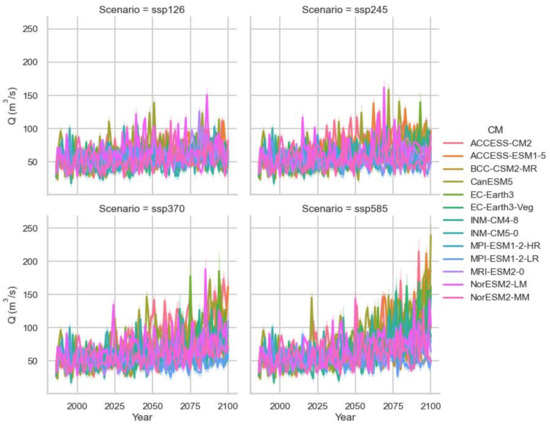
Figure 8.
Inter-annual variation of simulated streamflow under four SSPs forced with different climate models.
Figure 9 shows the projected monthly streamflow variation under four SSPs across the historical, near-term timeframe, and long-term timeframe periods. The uncertainty spread shows the variation projected by the selection of bias correction methods. The range of variability shown by the bias correction methods was not so large compared to the mean values. During both the near-term timeframe and long-term timeframe periods, the projected monthly streamflow was larger than in the historical period. Also, a clear increasing tendency of streamflow could be seen throughout the year. However, the magnitude of variation varied from month to month. As anticipated, the absolute values were higher during the rainy season compared to other seasons. The following section delves into the percentage deviation relative to monthly streamflow during the historical period.
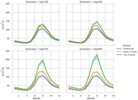
Figure 9.
Monthly variation in simulated streamflow during the historical, near-term timeframe, and long-term timeframe periods, showing the uncertainty related to bias correction methods.
Regarding the average streamflow during two future periods, a clear higher streamflow was projected in the long-term timeframe than sooner. The results suggested that streamflow in the long-term timeframe was projected to be higher than in the near-term timeframe, while the near-term timeframe was expected to have greater streamflow compared to the historical period. Overall, the pattern of monthly variation (i.e., intra-annual variation or seasonality) appeared to remain consistent across the future periods, resembling the patterns observed during the baseline period. A shift in the monthly hydrological regime was not projected with the analyzed selected thirteen climate models under all four SSPs. July and August are two months with high streamflow, and December to February are winter months with low streamflow. Under the two favorable circumstances of SSP 126 and SSP 245, the likely shifts in monthly streamflow were not that substantial compared to those under SSP 370 and SSP 585.
Figure 10 shows the projected monthly streamflow variation under four SSPs during the historical, near-term timeframe, and long-term timeframe periods, like Figure 9 However, the uncertainty spread in Figure 9 shows the variation projected by the selection of climate models. The range of variability shown by the selection of climate models was quite large compared to the mean values and sizeable to the range of variability shown by the bias correction methods. Therefore, the choice of climate models is crucial for conducting climate change assessments. Multiple criteria are necessary in selecting climate models to decrease the associated uncertainties with individual climate models.
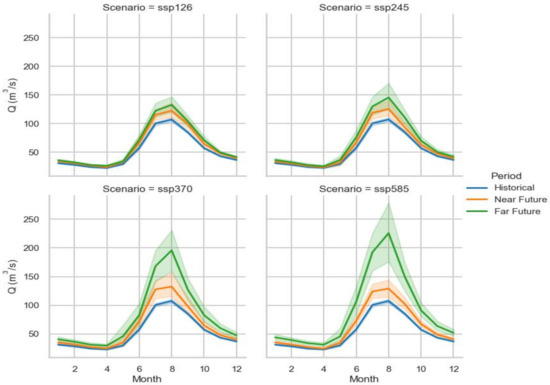
Figure 10.
Monthly variation of simulated streamflow during the baseline, near-term timeframe, and long-term timeframe periods, showing the uncertainty related to the selection of climate models.
As discussed earlier, during both the near-term timeframe and long-term timeframe periods, the projected monthly streamflow was larger than in the historical period. Also, a clear increasing tendency of streamflow could be seen throughout the year, meaning all twelve months. As discussed earlier, the magnitude of variation varied from month to month. As expected, the absolute values were higher in the monsoon season than in other seasons.
2.4.4. Projected Streamflow Deviation
Throughout the year, meaning all twelve months, streamflow was expected to rise during the future periods with respect to the historical period. A higher percentage increment was projected during the rainy season (June through August). During the near-term timeframe period, under SSP 126 and SSP 245, the percentage increment was around +20%, whereas under SSP 370 and SSP 585, the percentage increment was around +30% for the high flow season. The range of individual climate models varied greatly from less than 10% to up to 40–50% during the near-term timeframe period.
Similarly, during the long-term timeframe period, under SSP 126 and SSP 245, the percentage increment was below + 40%, see Supplementary Section Figure S11. By contrast, under SSP 370 and SSP 585, the percentage increment was greater than +60% for the high-flow season. Individual climate models varied comparatively more than during the near-term timeframe period. The ranges varied from less than 20% to 100% during the long-term timeframe period under different SSPs. According to the ensemble of thirteen climate models, the projected deviation on a monthly scale for two future periods is computed. Table 4 provides a synopsis of the projected monthly deviation for two future periods under four SSPs.
Table 4.
Monthly percentage deviation of projected streamflow relative to the historical baseline period (1986–2014).
During the near-term timeframe period (2031–2060), streamflow in November to March was projected to increase by around ten percent more than in the historical period. Higher SSPs projected even up to 13%. The deviation in April was projected to be the least, around 5 to 7% more than in the historical period. A greater increase was projected in the remaining months. Especially, higher increments were projected in June to August. Thus, the likelihood of flooding and higher discharge was high in the coming days. As a greater streamflow than the design discharge is not useful for water resource projects like irrigation, hydropower, or water supply, flooding discharge should be well designed for safe passage. Otherwise, these extreme events could damage water resource projects.
Similarly, during the long-term timeframe period (2071–2100), see Supplementary Section Figure S12. streamflow in November to April was projected to increase by less than twenty percent under two lower SSPs and up to 40% under two higher SSPs than in the historical period. Streamflow in the remaining months was projected to increase sharply. Especially, substantially higher increments were projected from June to August. Thus, the likelihood of flooding and higher discharge was even higher during the late century. If water resource projects are to be designed for the next 80 years, by the end of the period, managing the likelihood of higher streamflow and peak discharge will be crucial. Under the highest warming scenarios, deviations exceeding 100% were projected compared to the past stage.
3. Results
The performances of three hydrological models—HBV, HEC-HMS, and SWAT—were evaluated in the Kankai River Basin, focusing on calibration, parameter sensitivity, and overall model accuracy. Calibration processes for each model revealed distinct characteristics regarding parameter optimization and model performance
3.1. Hydrological Model Results
3.1.1. HBV Model
The optimization process adjusted one parameter at a time, while keeping all other parameters constant during the calibration phase. This one-dimensional optimization was iteratively repeated for a total of nineteen parameters. Rain Correction (PKRORR), Elevation Correction (HPKORR), Evaporation (LP), Fast Drainage Coefficient (KUZ2), Slow Drainage Coefficient (KUZ1), Threshold (UZ1), and Threshold Rain/Snow (TX) were found to be most sensitive for the study area. The optimization simulation was conducted within each parameter’s defined range, reflecting their physical properties. Numerous researchers have tested the HBV model, demonstrating its effectiveness in high mountain regions.
The HBV model differs from other simple hydrological models by its ability to incorporate threshold temperature, precipitation, snow, glacier dynamics, and soil processes while providing lead-time runoff forecasts. See Supplemental Material at S1 for more about the model. Its snow module employs the degree-day method to simulate snow accumulation and melting. However, the contribution of snow in the selected study area was minimal. For groundwater flow representation, three linear reservoir equations were utilized, with parameter ranges spanning from the lowest to the highest default values. During model calibration, the sensitive parameter ranges identified in previous studies were applied. Table 5 presents a list of parameters and their calibrated values for the study area. Figure 11 shows the performance of the HBV model on a daily scale.
Table 5.
Calibrated parameters of the HBV model for the study area.

Figure 11.
Comparison plots of daily observed and simulated flows for HBV model in the calibration (2005–2008) and validation (2009–2011) periods.
Overall, the highest runs were not taken with the model. However, the temporal variation and rainfall response processes were well captured with good agreement. Looking at the scatter plots, both under- and over-estimations could be noticed. Under-estimation was more noticeable for bigger discharge, whereas over-estimation was noticeable for lower discharge. In general, the volume was well captured, indicating that the HBV model was applicable when the interest was water volume rather than exact mimicking peak and lean flows.
3.1.2. HEC HMS Model
Manual and automatic methods were used in the optimization, and the Simplex method was found to be suitable for auto-calibration and is recommended for results by auto-calibration. Such auto-optimization was performed for fourteen parameters, as shown in Table 6. K, X, Number of Steps, and Recession factor were more sensitive, respectively. The optimization of the simulation was conducted within each parameter’s specified range, adhering to the model’s technical reference guidelines. The HEC-HMS model stood out from other simple models due to its ability to simulate peak values across various time scales, from yearly to hourly. See Supplemental Material at S2 for more about the model. Additionally, the selected research area exhibited higher flow rates despite receiving less rainfall compared to other basins. So, the current setup with daily simulations performed relatively better.
Table 6.
Calibrated parameters of the HECHMS model for the study area.
Figure 12 illustrates the results of the HEC HMS model at both daily and monthly scales. While the model struggled to accurately capture peak flow, it outperformed the HBV model in this regard. Similar to the HBV model, the HEC-HMS model effectively captured the temporal variation and rainfall response processes, showing good agreement. Scatter plots revealed both under- and over-estimations, with over-estimation being particularly notable. However, the model accurately represented the overall volume. In conclusion, the HEC-HMS model appeared to be more reliable for the Kankai River Basin, especially when focusing on total water volume and the magnitude of both higher and lower flows.
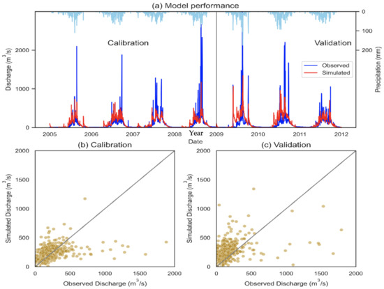
Figure 12.
Comparison plots of regular witnessed and simulated flows for the HEC-HMS model in the calibration (2005–2008) and validation (2009–2011) periods.
3.1.3. SWAT Model
Twenty-one input parameters were selected referring to the literature and published studies across Nepal. At first, considering the streamflow during the calibration period, 500 simulations were performed with 21 parameters. Then, another 500 simulations were performed with the revised range of these parameters, meaning 1000 simulations. This study found twelve sensitive parameters with p-values ≤ 0.05 (i.e., highly sensitive). The two-step process helped to fine-tune the range of sensitive parameters and understand the level of sensitivity. The most subtle parameters with p-values ≤ 0.1 [34] are shown in Table 7. NSE was chosen as an impartial function because it has many applications.
Table 7.
Calibrated sensitive parameters of the SWAT model.
GW_DELAY, RCHRG_DP, GWQMN, GW_REVAP, and ALPHA_BNK were recognised as important parameters for the river basin. These parameters modulate the base flow and groundwater. ALPHA-BNK, the baseflow alpha factor for bank storage (in days), characterizes the bank storage recession curve. Higher ALPHA_BNK values flatter the recession. If no value is entered, it is normally set to the same value as ALPHA_BF of the groundwater (gw) parameter CN2. The initial SCS curve numbers for moisture condition II (CN2) and LAT_TIME (lateral flow travel time in days) are equally sensitive parameters. CN2 depends on factors such as soil permeability, land use, and prior soil moisture conditions. LAT_TIME is the lateral flow travel time. These two parameters dictate the rainfall–runoff process. A few constraints that are meaningfully subtle to the streamflow in the Kankai River Basin are SOL_AWC and CANMX. SOL_AWC is the available water capacity of the soil (in mm water/mm soil). It is the difference between the water content at field capacity and the permanent wilting point. CANMX is the maximum canopy storage (in mm water), significantly affecting infiltration, surface runoff, and evaporation. CH_K2 and CH_N2 are the hydraulic conductivity and roughness coefficients, respectively, which are dependent on the physical properties of the soil type, LULC, and topography. See Supplemental Material S3 for more about the model.
Figure 13 presents the temporal variation in simulated streamflow at two ungauged locations (i.e., Kankai River Basin outlet and Kankai Irrigation Project Intake). These simulated results were derived from the calibrated model at the Mainachuli station. The green spread shows the 95 ppu based on the range of selected parameters and their ranges forced with hundreds of simulations.
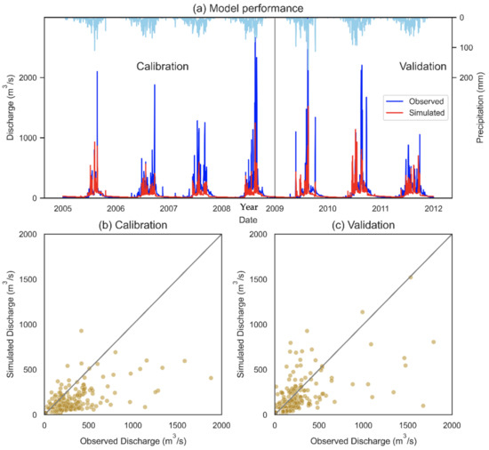
Figure 13.
Similarity plots of daily detected and replicated flows of SWAT model. Note: Model performance of SWAT at the Mainachuli hydrometric station on a daily scale during the calibration (2005–2008) and validation (2009–2011) periods.
3.2. Comparison of Three Hydrological Models
The intricacy of a watershed, along with the sensitivity of hydrological modeling parameters, inputs, and observed data to ambiguity, necessitates that researchers test the hydrological model through calibration and validation processes to assess its suitability [36]. This section provides the quantification of the model performance of three hydrological models in Figure 14. On a daily scale, looking at NSE and R2 values, none of the three models were ideal. For example, the HBV model showed NSE and R2 values of approximately 0.68 and 0.58 during calibration and 0.76 and 0.66 during validation, respectively; the HEC HMS model showed NSE and R2 values of approximately 0.67 and 0.71 during the calibration phase and 0.65 and 0.71 during the validation phase, respectively; and the SWAT model showed NSE and R2 values of approximately 0.79 and 0.83 during calibration and 0.75 and 0.81 during validation, respectively. These values indicated that the HBV model performance was inferior to that of the SWAT and HEC HMS models. The results indicated that the SWAT model was more applicable among them.

Figure 14.
Summary of model performance metrics of three hydrological models’ performance metrics for three hydrological models (HBV, HEC HMS, and SWAT) on a daily scale.
When comparing model accuracy and parameter sensitivity, the SWAT model emerged as the most suitable for the Kankai River Basin, particularly for assessing water volume and understanding groundwater processes [37]. Despite the HEC-HMS model’s better performance in simulating peak flow, SWAT’s superior calibration results and ability to handle agricultural processes made it the optimal choice for this study. The HBV model, though effective in snow-fed basins [35], was less accurate in this context due to its weaker performance in modeling rainfall-driven runoff and flow dynamics. Therefore, based on the overall performance metrics, SWAT was selected as the optimal hydrological model for the Kankai River Basin.
3.3. Model Calibration and Parameter Sensitivity
In the HBV model, 19 parameters were calibrated, with the key sensitive parameters identified as Rain Correction (PKRORR), Elevation Correction (HPKORR), Evaporation (LP), and Drainage Coefficients (KUZ1, KUZ2). The calibration results indicated good performance in capturing temporal variation and rainfall–runoff processes, although there were some discrepancies in peak and lean flow estimation. Under-estimation of high discharge and over-estimation of low flow were noted. Despite these errors, the volume of streamflow was well represented, making the HBV model suitable for volume-focused assessments.
The HEC-HMS model, using both manual and automatic optimization methods, focused on fourteen parameters, with the most sensitive being the Recession Factor, K, and X. The model exhibited a stronger ability to simulate peak flow compared to HBV, although it still showed some over-estimations, particularly in low-flow events. Despite challenges in accurately capturing peak flow, HEC-HMS effectively modeled the temporal flow variations, making it more reliable for scenarios requiring accurate peak flow predictions.
The SWAT model calibration involved 21 parameters, with twelve parameters identified as highly sensitive. These included groundwater parameters like GW_DELAY, RCHRG_DP, and baseflow factors like ALPHA_BNK. The two-step calibration process fine-tuned the parameter ranges and produced simulations that effectively captured the temporal variation in streamflow at multiple locations within the basin. Particularly notable was SWAT’s ability to model baseflow, groundwater processes, and its suitability for the agricultural landscape of the Kankai River Basin.
3.4. Bias Correction and GCM Model Selection
To ensure the reliability of the meteorological inputs, bias correction methods were applied to the GCM data. Given the inherent biases in GCM simulations, especially in precipitation and temperature predictions, bias correction was necessary to adjust the GCM outputs to better match observed data at the local scale. The quantile mapping method was selected as the primary bias correction technique. This method is known for its ability to preserve the statistical properties of the data, particularly the tail ends of the distribution, which is crucial for hydrological modeling in regions with significant rainfall variability. See Supplemental Material at S5 for more about bias correction of models.
For the GCM selection, several models were considered based on their historical performance and their ability to represent climate dynamics in the region. The HadGEM2-ES and MPI-ESM-LR models were selected for their relatively better representation of South Asia’s climate dynamics in past simulations. These models offer a range of projections under different emissions scenarios (RCP 4.5 and RCP 8.5), which are commonly used to assess future climate scenarios.
3.5. Downscaling GCM Models to Station Scale
Since GCMs operate at a global scale, downscaling was necessary to bring the GCM outputs to the local scale of the Kankai River Basin. Statistical downscaling was applied to the GCM data to convert coarse-scale outputs to finer spatial resolutions. The method used was the local intensity scaling (LIS), which adjusts the distribution of precipitation intensities and temperature values based on historical data from local weather stations. This approach ensures that the downscaled data better reflects the local climatology, thus improving the accuracy of the hydrological model simulations.
Downscaled data from the selected GCMs were then aggregated into daily meteorological inputs (precipitation, temperature, humidity, wind speed, and solar radiation) at a spatial resolution matching the scale of the SWAT model’s required inputs. This downscaling process was critical in providing reliable inputs for hydrological simulations.
3.6. Application of Multiple GCM Meteorological Data to SWAT
The downscaled meteorological data from multiple GCMs were used as inputs to the SWAT model to assess the range of potential future hydrological responses under different climate scenarios. The use of multiple GCMs allowed for a more comprehensive analysis of climate uncertainty and provided insights into the potential variability in streamflow and other hydrological processes.
In the SWAT model, inputs such as precipitation and temperature were modified based on the downscaled data from each GCM. For each GCM, simulations were conducted for multiple future periods (e.g., 2025–2050, 2050–2075, 2075–2100) under different emission scenarios (RCP 4.5 and RCP 8.5). The SWAT model was calibrated using observed streamflow data for the historical period (2005–2011) before applying future GCM projections to simulate the hydrological impacts of climate change.
3.7. Use of Ensemble Averaging of Multiple GCMs
To further reduce the uncertainty associated with using a single GCM projection, ensemble averaging of multiple GCM outputs was employed. This method involves combining the results from several GCMs to provide a more robust and reliable estimate of future climate conditions. By averaging the projections of multiple models, the influence of individual model biases is minimized, and a range of possible future outcomes is obtained.
Ensemble averaging was applied to the temperature and precipitation data derived from the downscaled GCM outputs. The ensemble mean was then used as the primary input for hydrological simulations in SWAT. This approach allowed for a more balanced representation of future climate conditions, ensuring that the hydrological modeling results were not overly dependent on the assumptions of any single model.
3.8. Model Performance Evaluation
In terms of model performance, the SWAT model demonstrated the highest accuracy across both calibration and validation phases, with the highest NSE and R2 values—0.79 and 0.83 during calibration and 0.75 and 0.81 during validation, respectively. The HEC-HMS model followed, with NSE and R² values of 0.67 and 0.71 during calibration and 0.65 and 0.71 during validation, respectively. The HBV model had the lowest performance metrics, with NSE and R² values of 0.68 and 0.58 during calibration and 0.76 and 0.66 during validation, respectively. These results highlighted SWAT’s superior ability to model the temporal streamflow dynamics in the Kankai River Basin.
Although none of the models perfectly captured peak flows, all three models successfully simulated the overall volume of streamflow. Notably, the SWAT model’s performance was more consistent across both high and low flows, making it the most reliable for water availability assessments in the study area. By comparison, the HEC-HMS model performed better in simulating peak flow, while HBV was more suited to snow-fed basins, which was not the case for the Kankai River Basin.
4. Discussion
4.1. Interpretation and Analysis of Results
The findings of this study provide a comprehensive assessment of flow alterations in the Kankai River Basin under changing climate scenarios using three hydrological models: HBV, HEC-HMS, and SWAT. The results indicate significant variations in flow patterns, with pronounced seasonal differences. The comparative analysis of model outputs suggests that HBV effectively captures base flow conditions, whereas HEC-HMS and SWAT provide better representations of peak flow events. The discrepancies observed between models highlight the inherent variability in hydrological predictions and emphasize the necessity of multi-model approaches for robust water resource management.
The SWAT model, in particular, exhibited higher accuracy in simulating groundwater interactions and long-term streamflow trends, which are crucial for sustainable water resource planning. On the other hand, HEC-HMS was more effective in modeling flood events and high-discharge periods, making it suitable for flood risk assessments. The HBV model, while effective in predicting overall streamflow patterns, exhibited limitations in capturing extreme hydrological events. These differences underscore the importance of using a combination of models to gain a comprehensive understanding of hydrological changes under climate variability.
4.2. Comparison with Existing Literature
The study’s findings align with previous research on flow alterations in similar medium-sized river basins in Nepal and other regions with comparable climatic conditions. Studies such as [38,39] emphasized the sensitivity of non-snow-fed rivers to precipitation variability and land-use changes. However, unlike these previous studies, our research uniquely integrates multiple hydrological models, enhancing the reliability of projections and reinforcing the importance of comparative model assessments in climate impact studies.
Furthermore, a previous study on Himalayan river basins [21] showed that increasing monsoonal precipitation and temperature rise are expected to exacerbate hydrological variability. Our results support these conclusions by projecting an increase in streamflow during monsoon months, raising concerns regarding future flood risks. Additionally, our findings suggest that changes in seasonal flow regimes could impact agricultural water availability, corroborating similar research conducted in the Gandaki and Koshi River Basins.
4.3. Analysis of Research Limitations
Despite the strengths of the study, several limitations must be acknowledged. First, the accuracy of hydrological models is contingent on the availability and quality of the input data, particularly precipitation and land-use data. Any uncertainties in these datasets may propagate through the models, affecting the reliability of results. Additionally, while the selected models are widely used, their inherent structural differences may introduce bias in certain hydrological components.
Another limitation stems from the assumptions embedded in climate models, particularly the bias correction methods used to adjust raw climate projections. While bias correction techniques enhance model accuracy, they may not fully eliminate uncertainties in future climate projections. Additionally, the study does not explicitly consider socioeconomic factors or water management policies, which may also influence flow regimes and require further investigation. Future studies should integrate socio-hydrological models to understand how water demand, land-use changes, and policy decisions interact with hydrological variability.
4.4. Contribution to Academic Knowledge
This research contributes to the academic discourse on hydrological modeling and climate change impacts by demonstrating the utility of multi-model approaches in assessing flow alterations in medium-sized river basins. By identifying the strengths and limitations of different hydrological models, this study provides valuable insights for future hydrological assessments and water resource planning.
Furthermore, this study highlights the importance of using CMIP6 climate models to simulate future hydrological conditions, offering a more refined approach to climate impact assessments compared to earlier studies based on CMIP5 models. The integration of multiple climate scenarios (SSP 126, SSP 245, SSP 370, and SSP 585) allows for a more detailed understanding of future hydrological extremes and their potential consequences.
The findings of this research are particularly relevant for policymakers and water resource managers in designing adaptive strategies for sustainable water management. The projected increase in streamflow during monsoon months underscores the need for improved flood control infrastructure and early warning systems. Conversely, the observed trends in dry season flow reductions highlight the importance of developing efficient irrigation strategies to mitigate water scarcity challenges.
Future research should focus on integrating socioeconomic factors and incorporating downscaled climate models for a more holistic understanding of climate-induced flow alterations. Additionally, further studies should explore nature-based solutions such as reforestation and wetland conservation to enhance water retention and mitigate flood risks. By bridging the gap between hydrological modeling and adaptive water management strategies, this research paves the way for more resilient water resource planning in Nepal and beyond.
5. Conclusions
This study comprehensively assessed the potential impacts of climate change on streamflow in the Kankai River Basin, Nepal, using a multi-model approach that integrated three hydrological models (HBV, HEC-HMS, and SWAT) with state-of-the-art CMIP6 climate models and Shared Socioeconomic Pathways (SSPs). The results indicated significant projected increases in streamflow across future periods, with notable variations depending on the emission scenarios and climate model uncertainties.
The SWAT model emerged as the most suitable tool for simulating streamflow in the Kankai River Basin, demonstrating superior performance in capturing both temporal dynamics and overall water volume. However, the study also highlighted the importance of selecting appropriate hydrological models based on the specific characteristics of the river basin, with HBV showing better applicability in snow-fed basins and HEC-HMS providing reliable peak flow predictions.
The climate model outputs revealed substantial increases in precipitation and temperature, particularly under higher emission scenarios (SSP 370 and SSP 585). These changes were projected to lead to a significant rise in streamflow, especially during the monsoon season (June–August), with potential implications for flooding and water resource management. The study emphasizes the necessity of robust bias correction techniques and multi-model ensembles to reduce uncertainties associated with individual climate models.
Overall, the findings suggested that future water availability in the Kankai River Basin will be characterized by increased streamflow, posing both opportunities and challenges for water resource projects, including irrigation, hydropower, and flood control. The projected changes highlight the need for adaptive management strategies and infrastructure planning to mitigate the impacts of extreme events and ensure sustainable water use in the region. Future research should focus on detailed assessments of individual climate models and their performance at the local scale, as well as exploring the combined effects of land use changes and climate variability on hydrological processes.
Supplementary Materials
The following supporting information can be downloaded at: https://www.mdpi.com/article/10.3390/w17070940/s1, S1: HBV model; S2: HEC-HMS model; S3: SWAT model; S4: CMIP6; S5: Bias Correction of Climate Models; Figure S1: Comparison of observed raw, and bias-corrected thirteen climate models’ precipitation; Figure S2: Comparison of observed raw, and bias-corrected thirteen climate models of the maximum temperature; Figure S3: Comparison of observed raw and bias-corrected thirteen climate models minimum temperature; Figure S4: Inter-annual variation of precipitation under four SSPs using different bias correction methods; Figure S5: Inter-annual variation of precipitation under four SSPs forced with different climate models; Figure S6: Inter-annual variation of Tmax under four SSPs using different bias correction methods; Figure S7: Inter-annual variation of Tmax under four SSPs forced with different climate models; Figure S8: Inter-annual variation of Tmax under four SSPs using different bias correction methods; Figure S9: Inter-annual variation of Tmin under four SSPs forced with different climate models; Figure S10: Inter-annual variation of simulated streamflow under four SSPs using different bias correction methods; Figure S11: Projected monthly deviation during the Near Future (2031–2060) expressed in percentage with respect to the Historical period (1986–2014); Figure S12: Projected monthly deviation during the Far Future (2071–2100) expressed in percentage with respect to the Historical period (1986–2014). References [40,41,42,43,44,45,46,47,48,49,50] are cited in Supplementary Materials.
Author Contributions
Conceptualization, M.S., R.P.S. and S.R.S.; Methodology, M.S., R.P.S. and S.R.S.; Software, M.S., R.P.S. and S.R.S.; Validation, M.S. and R.P.S.; Formal analysis, M.S. and S.R.S.; Investigation, M.S., R.P.S. and S.R.S.; Resources, M.S.; Data curation, M.S., R.P.S. and S.R.S.; Writing—original draft, M.S., R.P.S. and S.R.S.; Writing—review & editing, M.S. and R.P.S.; Visualization, M.S. and S.R.S.; Supervision, R.P.S.; Project administration, R.P.S. All authors have read and agreed to the published version of the manuscript.
Funding
This research received no external funding.
Data Availability Statement
The data will be made available upon reasonable request to the corresponding author.
Acknowledgments
Manan Sharma would like to express my sincere gratitude to Mao Jing Qiao, for his invaluable guidance, support, and encouragement throughout the preparation of this manuscript. His expertise, thoughtful feedback, and continuous mentorship have been instrumental in shaping the direction of this research. Manan Sharma is deeply grateful for his patience and dedication, which made this work possible.
Conflicts of Interest
The authors declare no conflicts of interest.
Abbreviations
The following abbreviations are used in this manuscript:
| ALOS | Advanced Land Observing Satellite |
| CIMP | Coupled Model Intercomparison Project |
| DEM | Digital Elevation Model |
| DHM | Department of Hydrology and Meteorology |
| EQM | Empirical Quantile Mapping |
| FDC | Flow Duration Curve |
| GCM | Global Climate Model |
| GHG | Green House Gas |
| GWRDB | Groundwater Resources Development Board |
| HBV | Hydrologiska Byråns Vattenbalansavdelning |
| HECHMS | Hydrologic Engineering Center’s Hydrologic Modeling System |
| HRU | Hydrological Response Unit |
| LS | Linear Scaling |
| LULC | Land Use Land Cover |
| MoEWRI | Ministry of Energy, Water Resources and Irrigation |
| MDD | Mean Daily Discharge |
| NSE | Nash-Sutcliffe Efficiency |
| PBIAS | Percentage Bias |
| PET | Potential Evaporation Transpiration |
| QM | Quantile Mapping |
| RCP | Representative Concentration Pathway |
| SOTER | Soil and Terrian Database |
| SMHI | Swedish Meteorological and Hydrological Institute |
| SSPs | Shared Socioeconomic Pathways |
| SWAT | Soil and Water Assessment Tool |
| USDA | United State Agriculture department |
| WRRDC | Water Resources Research and Development Centre |
Appendix A
Figure A1.
Comparison of observed and raw, and bias-corrected thirteen climate models precipitation using parametric simple linear transformation.
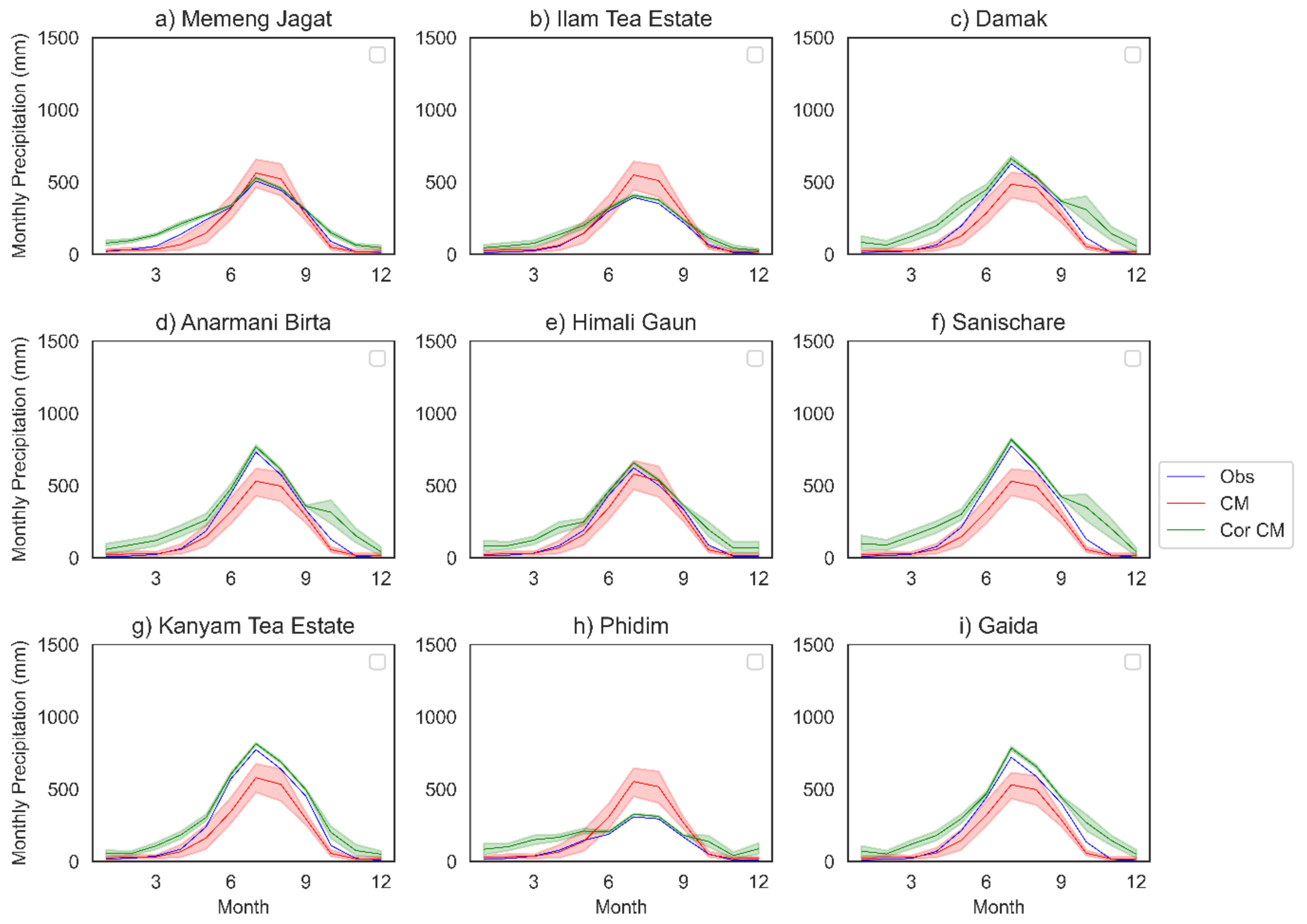
Figure A2.
Comparison of observed and raw, and bias-corrected thirteen climate models precipitation using parametric Exponential asymptote transformation.
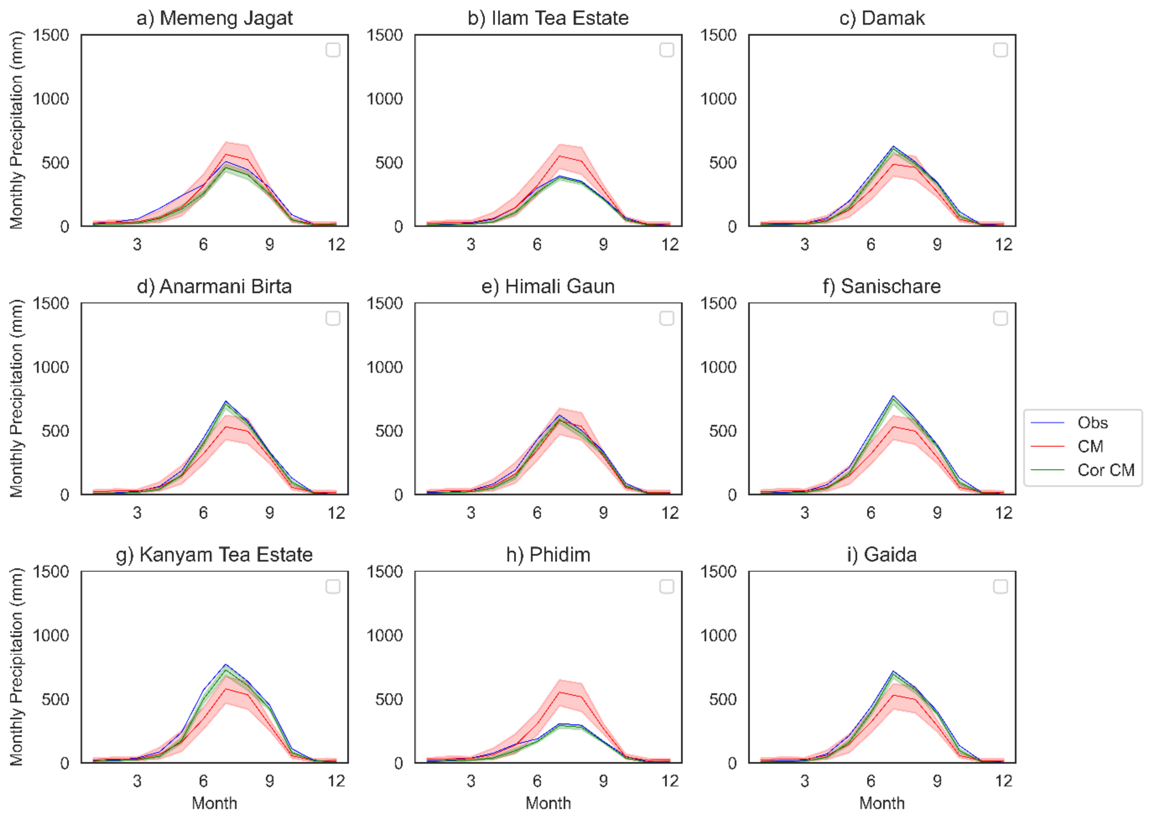
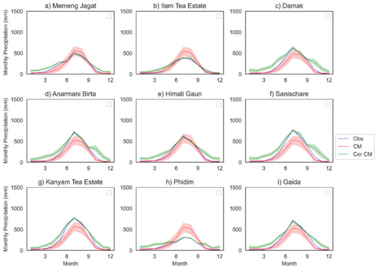
Figure A3.
Comparison of observed and raw, and bias-corrected thirteen climate models precipitation using nonparametric EQM transformation.
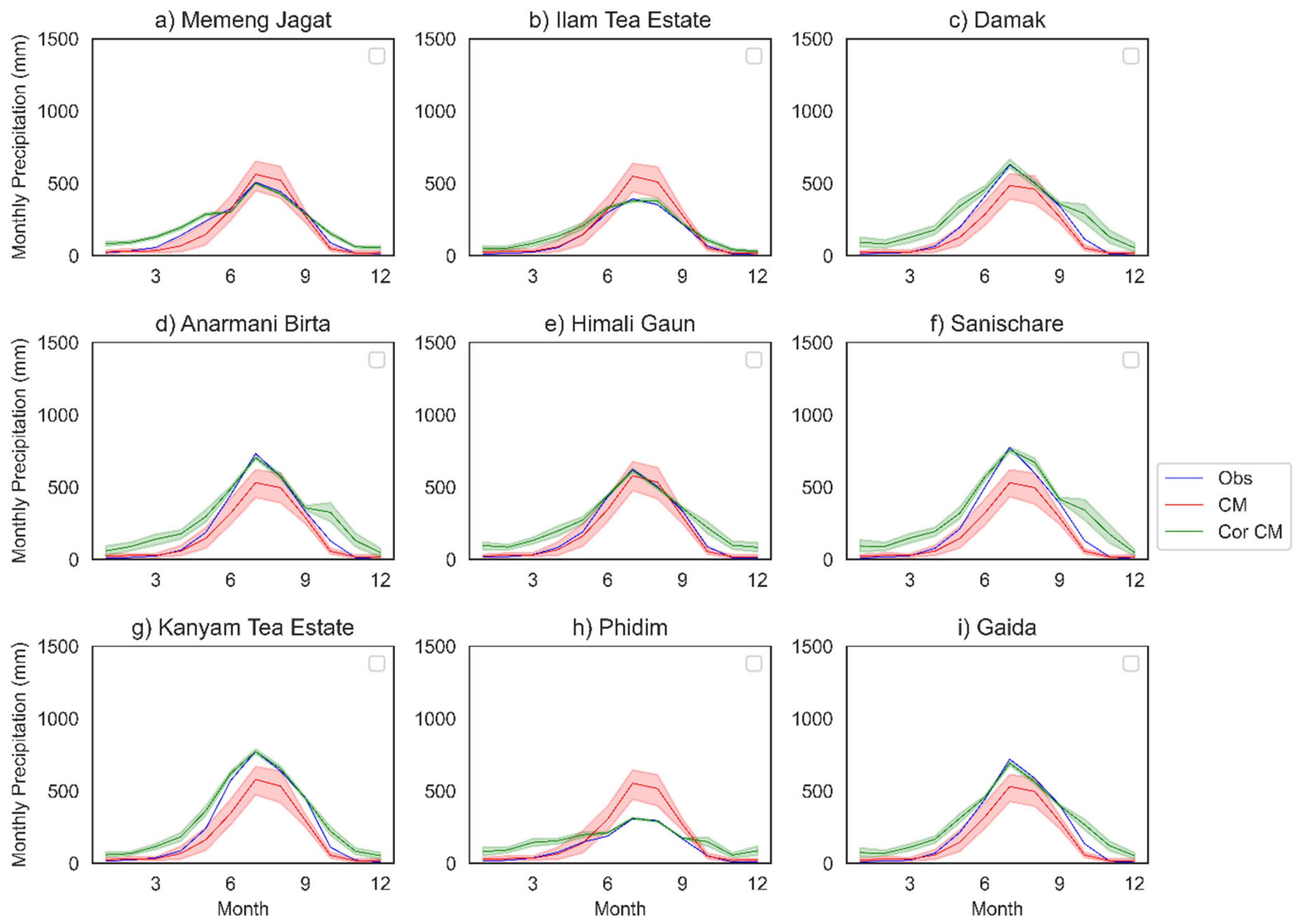
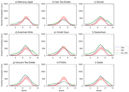
Figure A4.
Comparison of observed and raw, and bias-corrected thirteen climate models precipitation using nonparametric ERQM transformation.
References
- Wani, M.U.H.; Wani, S.M. Sustainability of Himalayan Environment: Issues and Policies. In Natural Resource Management: Ecological Perspectives; Springer Nature: London, UK, 2019; pp. 31–45. [Google Scholar]
- Gurung, S.B.; Sigdel, S.R.; Rokaya, M.B. Nepal: An Introduction, in Flora and Vegetation of Nepal; Springer: Berlin/Heidelberg, Germany, 2024; pp. 1–17. [Google Scholar]
- Shin, S.; Pokhrel, Y.; Talchabhadel, R.; Panthi, J. Spatio-temporal dynamics of hydrologic changes in the Himalayan river basins of Nepal using high-resolution hydrological-hydrodynamic modeling. J. Hydrol. 2021, 598, 126209. [Google Scholar]
- Joseph, G. Glaciers, Rivers, and Springs: A Water Sector Diagnostic of Nepal ©; World Bank: Washington, DC, USA, 2022. [Google Scholar]
- Gautam, D. Assessment of social vulnerability to natural hazards in Nepal. Nat. Hazards Earth Syst. Sci. 2017, 17, 2313–2320. [Google Scholar]
- Amadio, M.; Behrer, A.P.; Bosch, L.; Kaila, H.K.; Krishnan, N.; Molinario, G. Climate Risks, Exposure, Vulnerability and Resilience in Nepal; World Bank: Washington, DC, USA, 2023. [Google Scholar]
- National Planning Commission. Nepal: Experience, Gaps and Needs in Disaster Risk Reduction and Climate Change Adaptation Planning and Financing; National Planning Commission: Kathmandu, Nepal, 2015. [Google Scholar]
- Thapa, B.; Watanabe, T.; Regmi, D. Flood assessment and identification of emergency evacuation routes in Seti River Basin. Nepal Land 2022, 11, 82. [Google Scholar]
- Chhetri, R.; Pandey, V.P.; Talchabhadel, R.; Thapa, B.R. How do CMIP6 models project changes in precipitation extremes over seasons and locations across the mid hills of Nepal? Theor. Appl. Climatol. 2021, 145, 1127–1144. [Google Scholar]
- Adhikari, S.; Shrestha, D.; Nepal, B.; Chhetri, T.B.; Bhattarai, S. Identification of Summer Monsoon Onset over Nepal by using Satellite-Derived OLR Data. Jalawaayu 2022, 2, 19–32. [Google Scholar]
- Dhaubanjar, S.; Pandey, V.; Subedi, R. Water balance component analysis of a spring catchment of western Nepal. Banko Janakari 2021, 31, 23–32. [Google Scholar]
- Mousavi, S.J.; Abbaspour, K.C.; Kamali, B.; Amini, M.; Yang, H. Uncertainty-based automatic calibration of HEC-HMS model using sequential uncertainty fitting approach. J. Hydroinform. 2012, 14, 286–309. [Google Scholar]
- Wang, Y.; Wang, Y.; Wang, Y.; Li, C.; Ju, Q.; Jin, J.; Deng, X.; Sun, G.; Bao, Z. Applicability of the HBV model to a human-influenced catchment in northern China. Hydrol. Res. 2023, 54, 208–219. [Google Scholar] [CrossRef]
- Suryawanshi, V.; Honnasiddaiah, R.; Thuvanismail, N. Large-scale flood forecasting in coastal reservoir with hydrological modeling. Arab. J. Geosci. 2024, 17, 309. [Google Scholar]
- Nguyen, Q.A. Runoff Modeling of the Saugatucket River: An Application of HEC-HMS Software. Master’s Thesis, University of Rhode Island, Kingston, RI, USA, 2001. [Google Scholar]
- Chakraborty, S.; Biswas, S. Simulation of flow at an ungauged river site based on HEC-HMS model for a mountainous river basin. Arab. J. Geosci. 2021, 14, 2080. [Google Scholar]
- Pak, J.; Fleming, M.; Scharffenberg, W.; Ely, P. Soil erosion and sediment yield modeling with the hydrologic modeling system (HEC-HMS). In Proceedings of the World Environmental and Water Resources Congress 2008, Honolulu, HI, USA, 12 May 2008. [Google Scholar]
- Bai, Y.; Zhang, Z.; Zhao, W. Assessing the impact of climate change on flood events using HEC-HMS and CMIP5. Water Air Soil Pollut. 2019, 230, 119. [Google Scholar] [CrossRef]
- Arnold, J.G.; Srinivasan, R.; Muttiah, R.S.; Williams, J.R. Large area hydrologic modeling and assessment part I: Model development 1. JAWRA J. Am. Water Resour. Assoc. 1998, 34, 73–89. [Google Scholar] [CrossRef]
- Abbaspour, K.C.; Yang, J.; Maximov, I.; Siber, R.; Bogner, K.; Mieleitner, J.; Zobrist, J.; Srinivasan, R. Modelling hydrology and water quality in the pre-alpine/alpine Thur watershed using SWAT. J. Hydrol. 2007, 333, 413–430. [Google Scholar]
- Devkota, L.P.; Gyawali, D.R. Impacts of climate change on hydrological regime and water resources management of the Koshi River Basin, Nepal. J. Hydrol. Reg. Stud. 2015, 4, 502–515. [Google Scholar] [CrossRef]
- Ayele, G.T.; Teshale, E.Z.; Yu, B.; Rutherfurd, I.D.; Jeong, J. Streamflow and sediment yield prediction for watershed prioritization in the Upper Blue Nile River Basin. Ethiop. Water 2017, 9, 782. [Google Scholar]
- Pokhrel, B.K. Impact of land use change on flow and sediment yields in the Khokana Outlet of the Bagmati River, Kathmandu, Nepal. Hydrology 2018, 5, 22. [Google Scholar] [CrossRef]
- Lamichhane, S.; Shakya, N.M. Integrated assessment of climate change and land use change impacts on hydrology in the Kathmandu Valley watershed, Central Nepal. Water 2019, 11, 2059. [Google Scholar] [CrossRef]
- Sun, Y.; Bao, W.; Jiang, P.; Wang, X.; He, C.; Zhang, Q.; Wang, J. Development of dynamic system response curve method for estimating initial conditions of conceptual hydrological models. J. Hydroinform. 2018, 20, 1387–1400. [Google Scholar] [CrossRef]
- Lamichhane, M.; Mishra, Y.; Bhattarai, P. Assessment of future water availability and irrigation water demand under climate change in the Kankai River Basin, Nepal. J. Earth Sci. Clim. Change 2022, 13, 9. [Google Scholar]
- Gandhi, S.; Sarkar, B. Essentials of Mineral Exploration and Evaluation; Elsevier: Amsterdam, The Netherlands, 2016. [Google Scholar]
- Chaubey, I.; Cotter, A.S.; Costello, T.A.; Soerens, T.S. Effect of DEM data resolution on SWAT output uncertainty. Hydrol. Process. Int. J. 2005, 19, 621–628. [Google Scholar] [CrossRef]
- Uddin, K.; Shrestha, H.L.; Murthy, M.S.R.; Bajracharya, B.; Shrestha, B.; Gilani, H.; Pradhan, S.; Dangol, B. Development of 2010 national land cover database for the Nepal. J. Environ. Manag. 2015, 148, 82–90. [Google Scholar]
- Geza, M.; McCray, J.E. Effects of soil data resolution on SWAT model stream flow and water quality predictions. J. Environ. Manag. 2008, 88, 393–406. [Google Scholar]
- Dijkshoorn, K.; Huting, J. Soil and Terrain Database for Nepal; ISRIC–World Soil Information: Wageningen, The Netherlands, 2009; p. 21. [Google Scholar]
- Cook, B.I.; Mankin, J.S.; Marvel, K.; Williams, A.P.; Smerdon, J.E.; Anchukaitis, K.J. Twenty-first century drought projections in the CMIP6 forcing scenarios. Earth’s Future 2020, 8, e2019EF001461. [Google Scholar]
- Eyring, V.; Bony, S.; Meehl, G.A.; Senior, C.A.; Stevens, B.; Stouffer, R.J.; Taylor, K.E. Overview of the Coupled Model Intercomparison Project Phase 6 (CMIP6) experimental design and organization. Geosci. Model Dev. 2016, 9, 1937–1958. [Google Scholar]
- Abbaspour, K.C. SWAT calibration and uncertainty programs. A User Man. 2015, 103, 17–66. [Google Scholar]
- Lee, M.-H.; Bae, D.-H. Uncertainty assessment of future projections on water resources according to climate downscaling and hydrological models. J. Hydroinform. 2018, 20, 597–607. [Google Scholar]
- Gull, S.; Shah, S.R. Hydrological modeling for streamflow and sediment yield simulation using the SWAT model in a forest-dominated watershed of north-eastern Himalayas of Kashmir Valley, India. J. Hydroinform. 2022, volume, jh2022042. [Google Scholar]
- Sempewo, J.I.; Twite, D.; Nyenje, P.; Mugume, S.N. Comparison of SWAT and HEC-HMS model performance in simulating catchment runoff. J. Appl. Water Eng. Res. 2023, 11, 481–495. [Google Scholar]
- Subedi, S.R.; Lamichhane, M.; Dhungana, S.; Chalise, B.; Bhattarai, S.; Chaulagain, U.; Khatiwada, R. Assessing the impact of climate change on streamflow in the Tamor River Basin, Nepal: An analysis using SWAT and CMIP6 scenarios. Discov. Civ. Eng. 2024, 1, 135. [Google Scholar] [CrossRef]
- Dahal, P.; Shrestha, M.L.; Panthi, J.; Pradhananga, D. Modeling the future impacts of climate change on water availability in the Karnali River Basin of Nepal Himalaya. Environ. Res. 2020, 185, 109430. [Google Scholar]
- Ho, H.-C.; Chan, K.-C.; Chang, S.-H.; Huang, C.-C. Three-phase data augmentation for the prediction of sediment flux in mountain basins during typhoon events. J. Hydroinformatics 2023, 25, 1054–1071. [Google Scholar] [CrossRef]
- Arnold, J.G.; Moriasi, D.N.; Gassman, P.W.; Abbaspour, K.C.; White, M.J.; Srinivasan, R.; Santhi, C.; Harmel, R.D.; van Griensven, A.; van Liew, M.W.; et al. SWAT: Model Use, Calibration, and Validation. Trans. ASABE 2012, 55, 1509–1522. [Google Scholar] [CrossRef]
- Karakoyun, E.; Kaya, N. Hydrological simulation and prediction of soil erosion using the SWAT model in a mountainous watershed: A case study of Murat River Basin, Turkey. J. Hydroinformatics 2022, 24, 1175–1193. [Google Scholar] [CrossRef]
- Bhatta, B.; Shrestha, S.; Shrestha, P.K.; Talchabhadel, R. Evaluation and application of a SWAT model to assess the climate change impact on the hydrology of the Himalayan River Basin. CATENA 2019, 18, 104082. [Google Scholar] [CrossRef]
- Bista, S.; Singh, U.; Kayastha, N.; Ghimire, B.N.; Talchabhadel, R. Effects of source digital elevation models in assessment of gross runoff-river hydropower potential: A case study of West Rapti Basin, Nepal. J. Eng. Issues Solut. 2021, 1, 106–128. [Google Scholar] [CrossRef]
- Pandey, V.P.; Dhaubanjar, S.; Bharati, L.; Thapa, B.R. Spatio-temporal distribution of water availability in Karnali-Mohana Basin, Western Nepal: Hydrological model development using multi-site calibration approach (Part-A). J. Hydrol. Reg. Stud. 2020, 29, 100690. [Google Scholar] [CrossRef]
- Talchabhadel, R.; Aryal, A.; Kawaike, K.; Yamanoi, K.; Nakagawa, H.; Bhatta, B.; Karki, S.; Thapa, B.R. Evaluation of precipitation elasticity using precipitation data from ground and satellite-based estimates and watershed modeling in Western Nepal. J. Hydrol. Reg. Stud. 2021, 33, 100768. [Google Scholar] [CrossRef]
- Setegn, S.G.; Srinivasan, R.; Dargahi, B. Hydrological Modelling in the Lake Tana Basin, Ethiopia Using SWAT Model. Open Hydrol. J. 2008, 2, 49–62. [Google Scholar] [CrossRef]
- Bharati, L.; Gurung, P.; Maharjan, L.; Bhattarai, U. Past and future variability in the hydrological regime of the Koshi Basin, Nepal. Hydrol. Sci. J. 2016, 61, 79–93. [Google Scholar] [CrossRef]
- Pandey, V.P.; Dhaubanjar, S.; Bharati, L.; Thapa, B.R. Spatio-temporal distribution of water availability in Karnali-Mohana Basin, Western Nepal: Climate change impact assessment (Part-B). J. Hydrol. Reg. Stud. 2020, 29, 100691. [Google Scholar] [CrossRef]
- Talchabhadel, R.; Karki, R. Assessing climate boundary shifting under climate change scenarios across Nepal. Environ. Monit. Assess. 2019, 191, 520. [Google Scholar] [CrossRef] [PubMed]
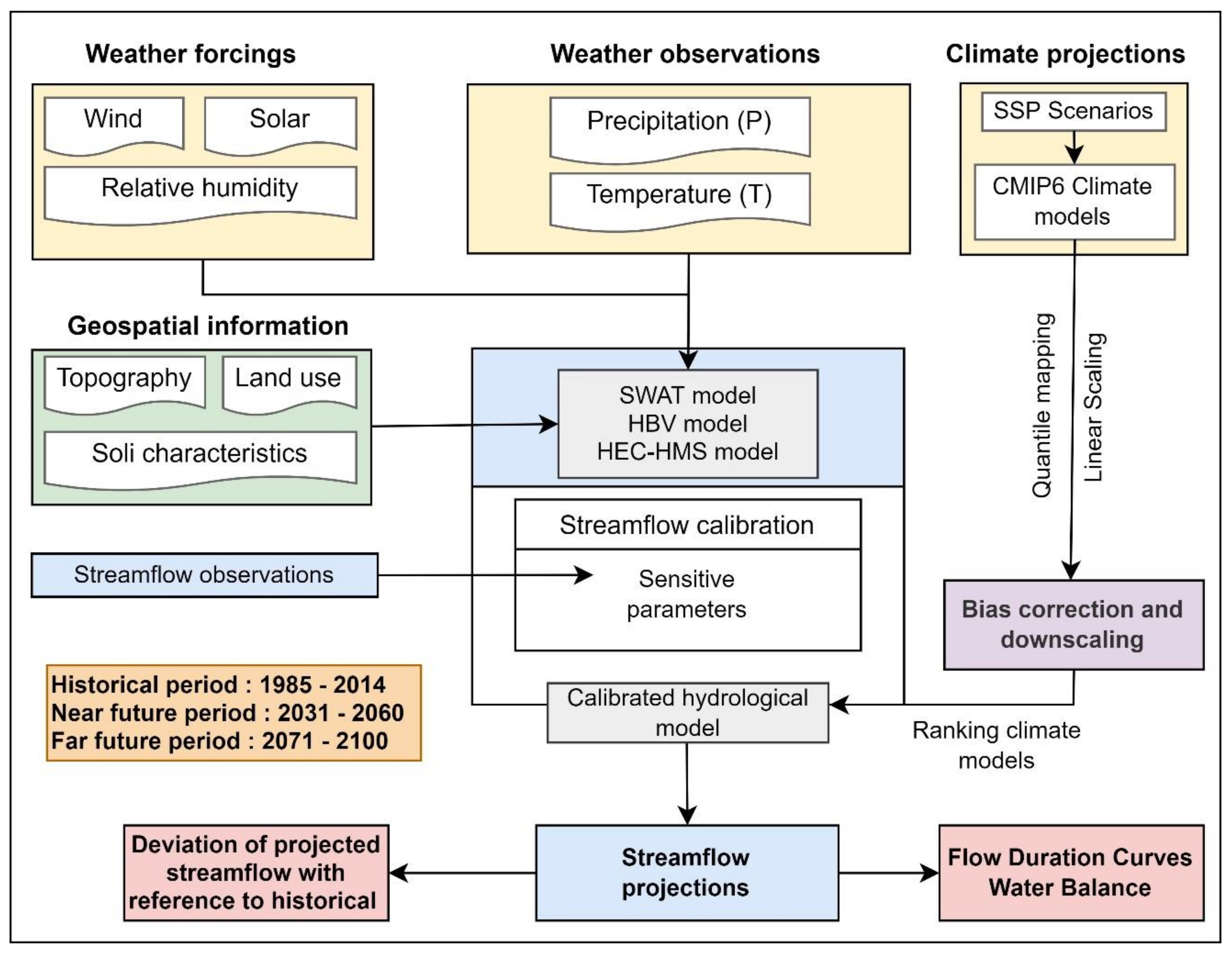
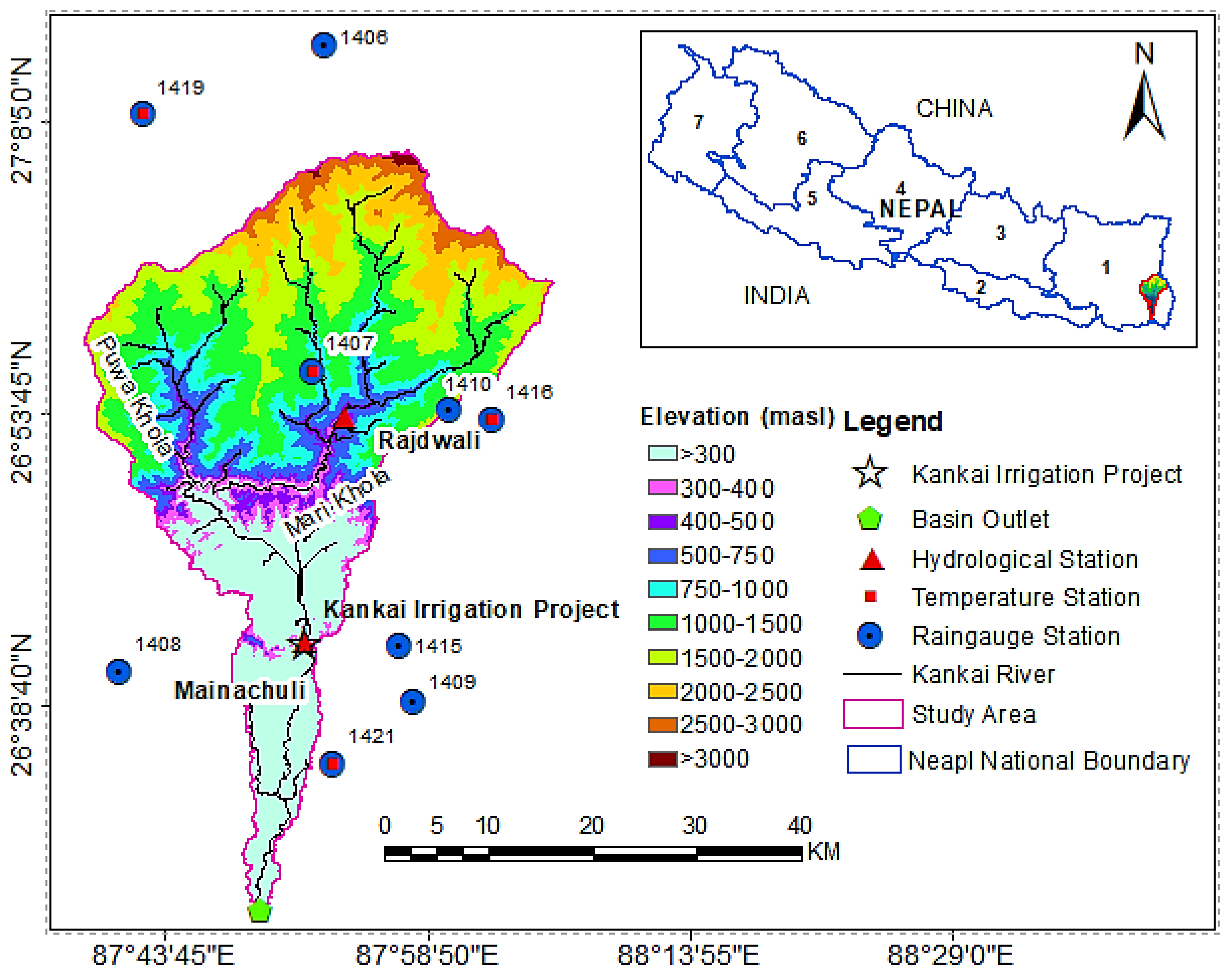

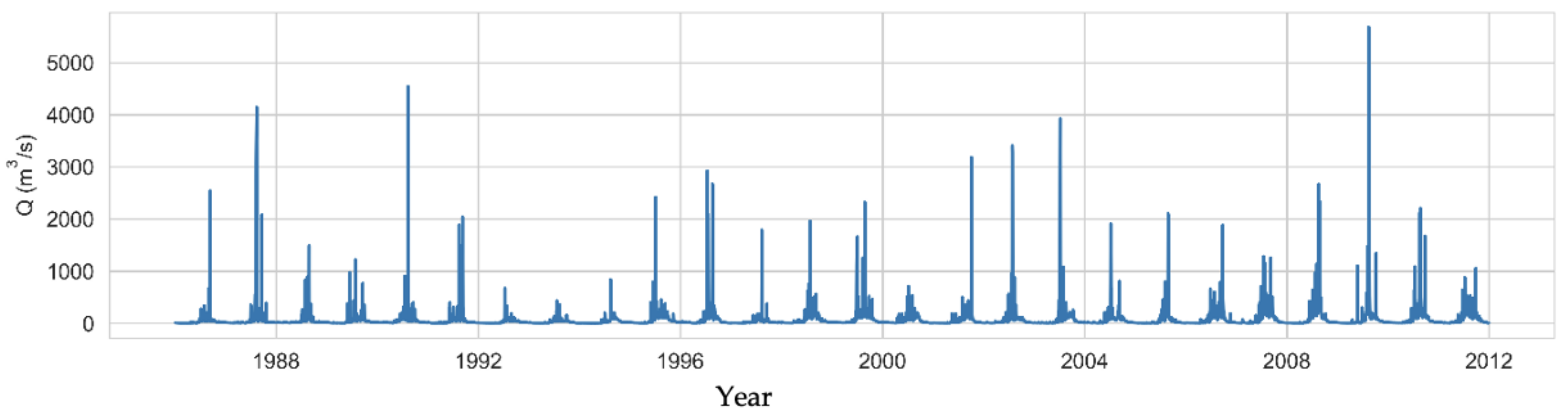
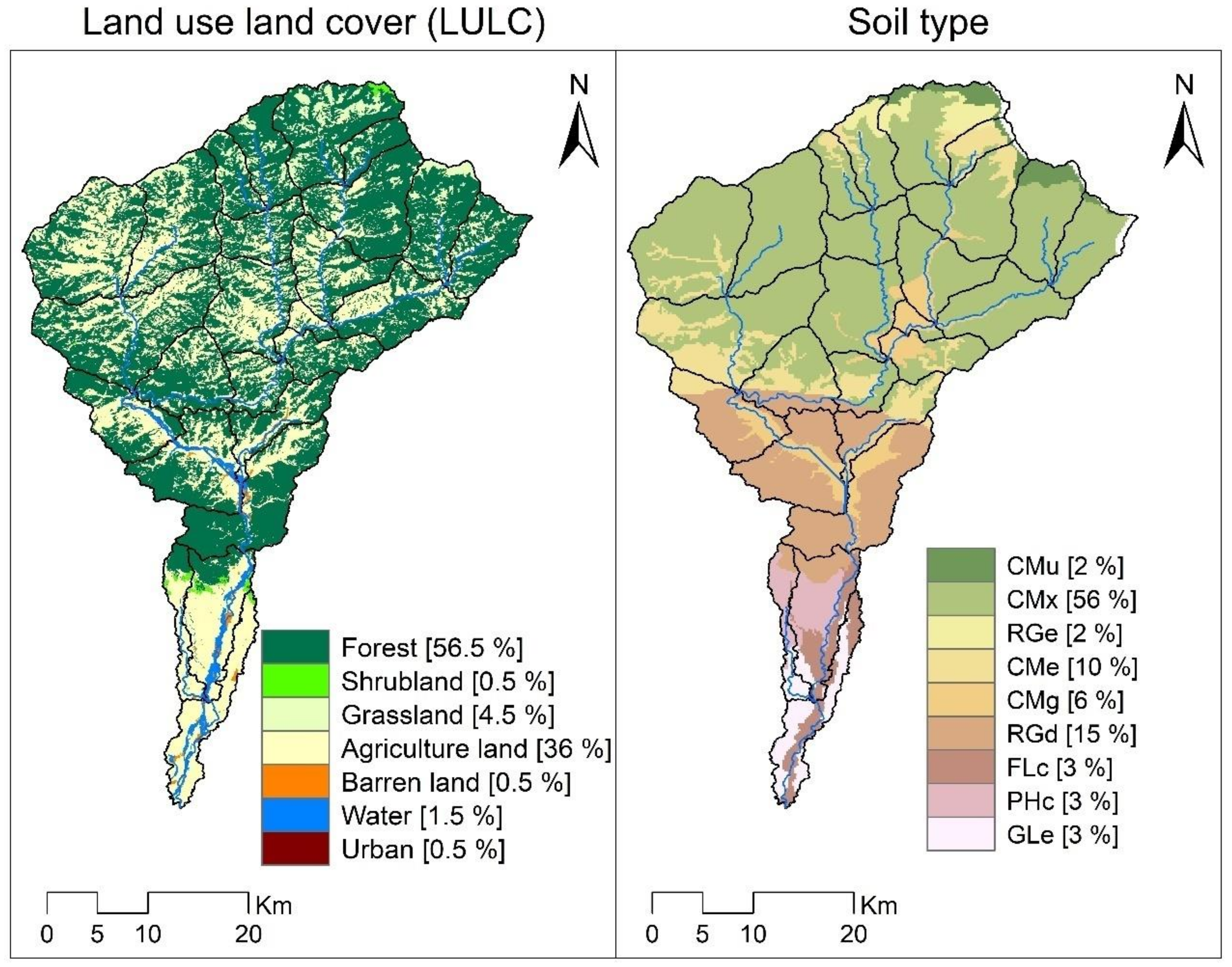
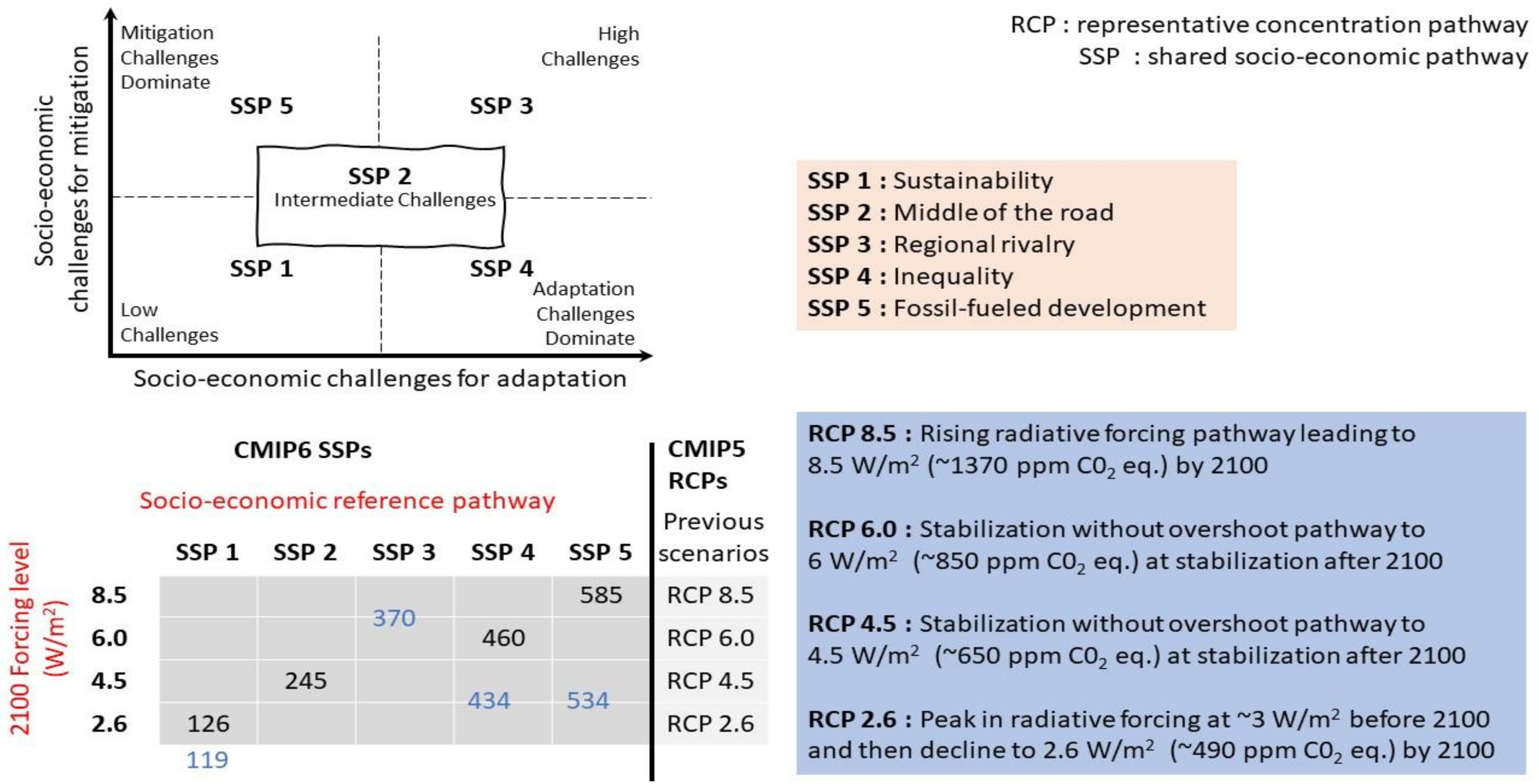
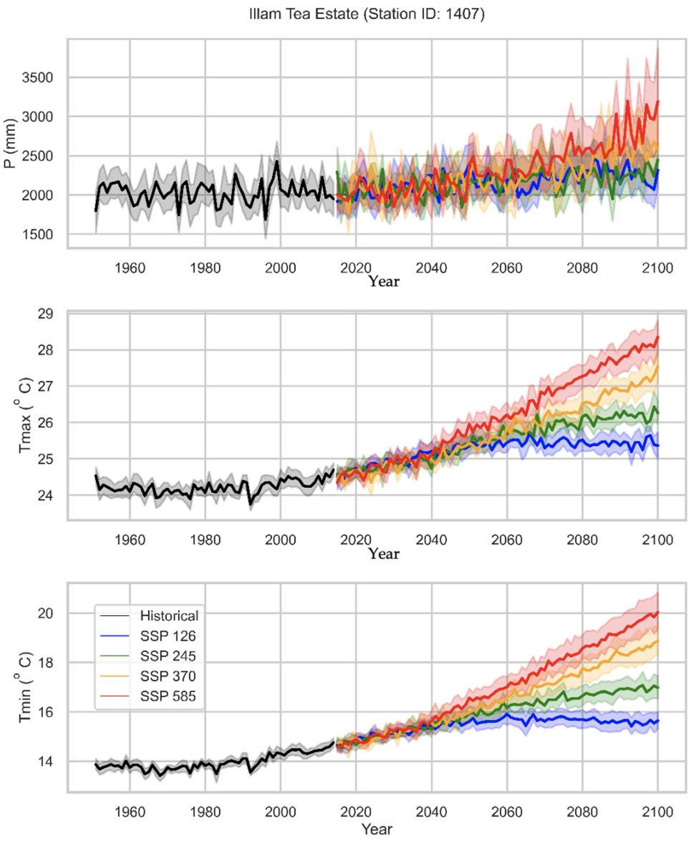

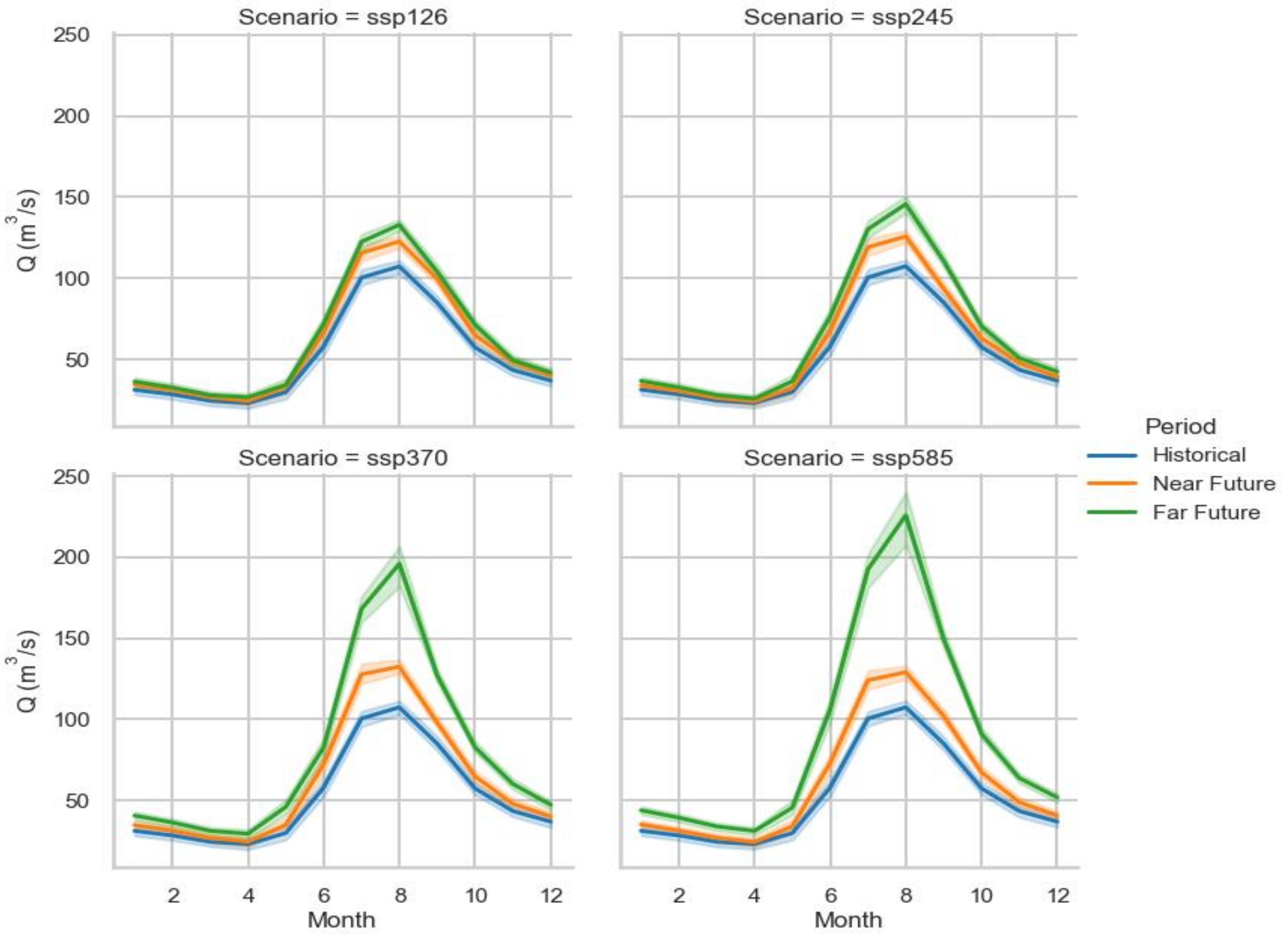
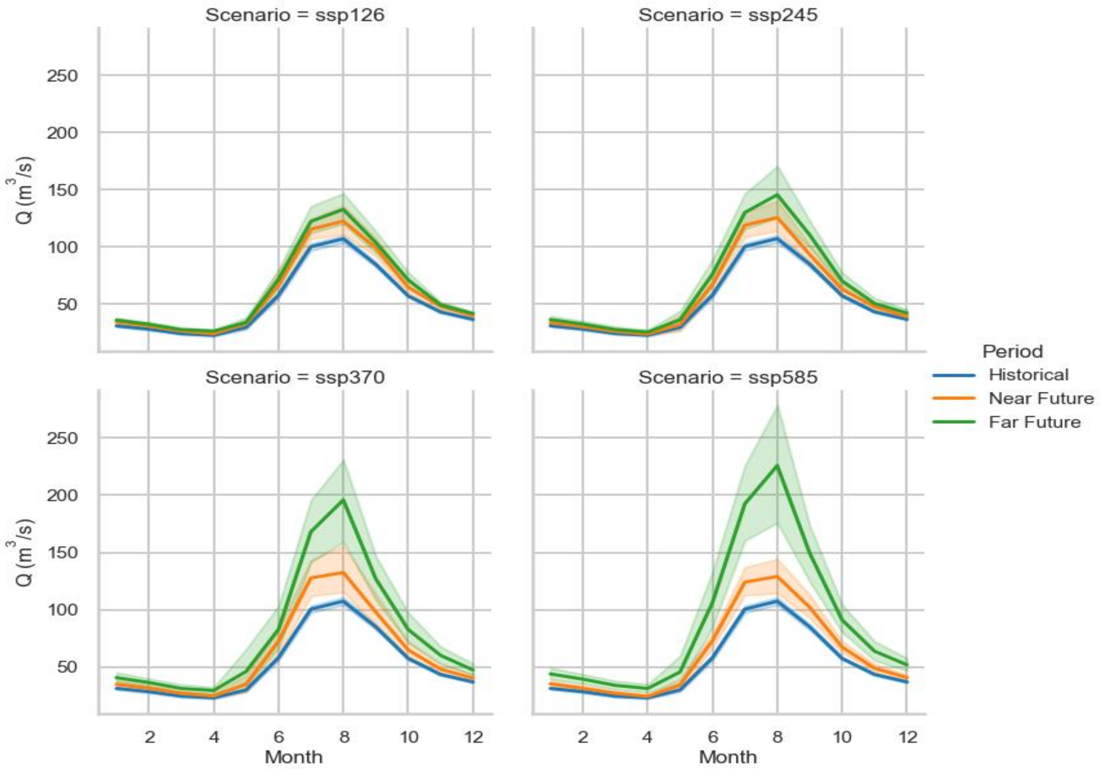
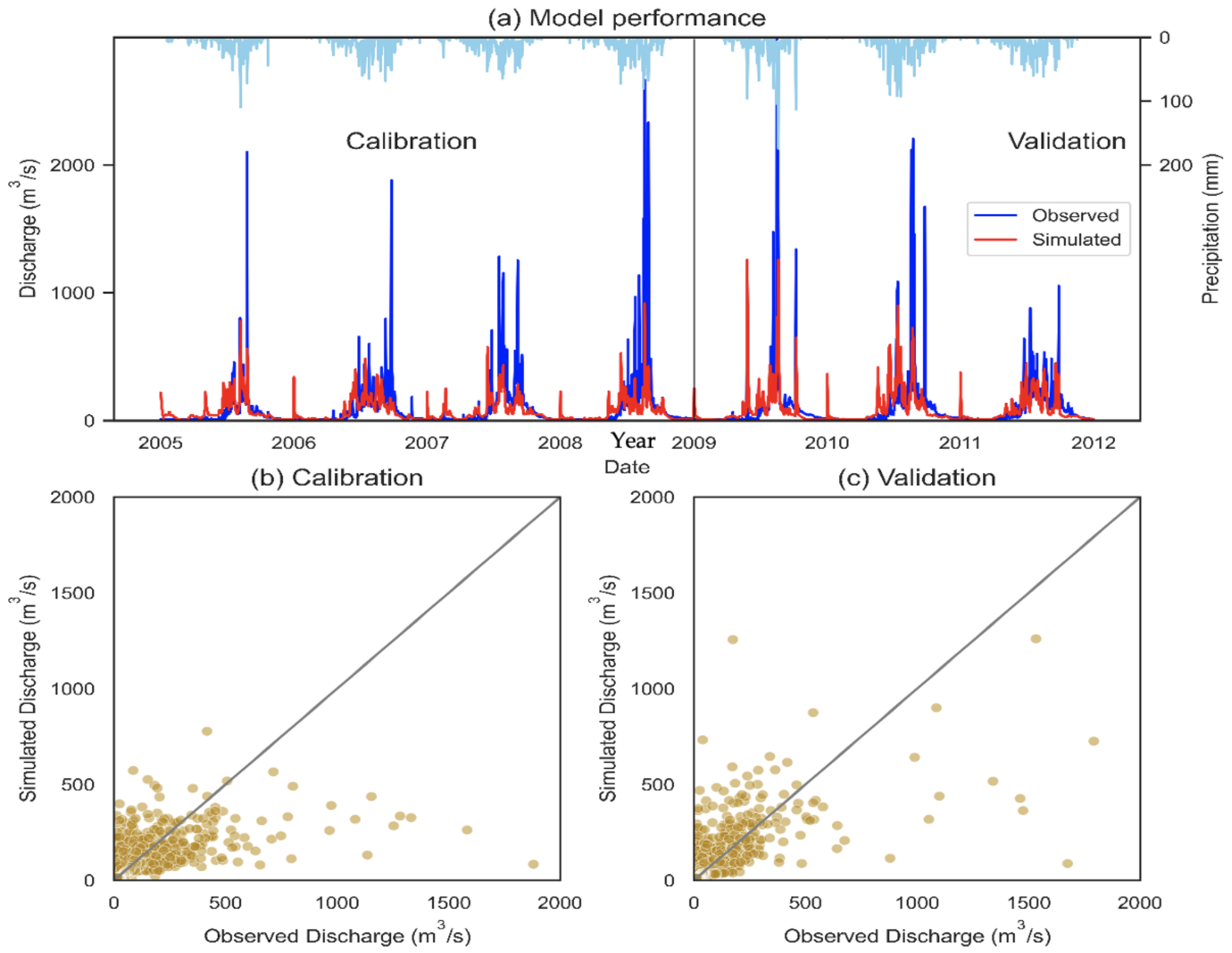
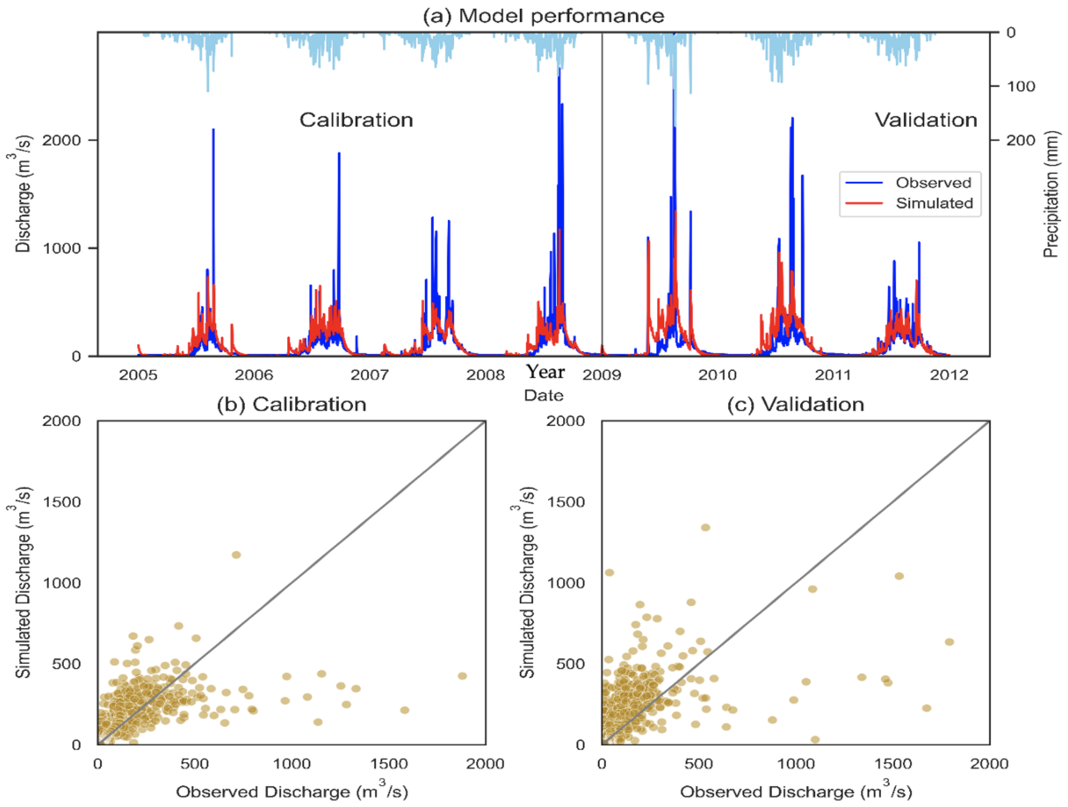

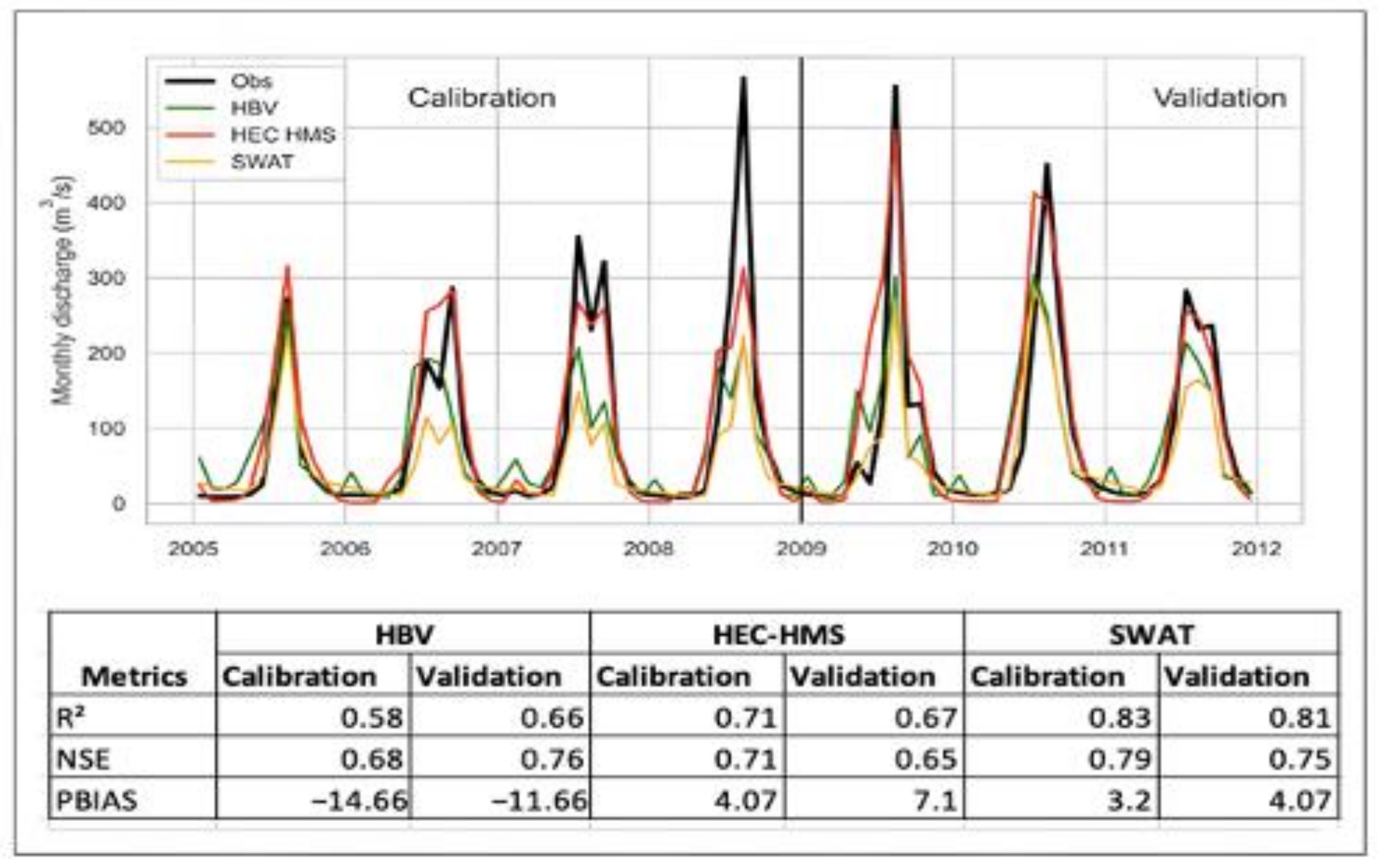
Disclaimer/Publisher’s Note: The statements, opinions and data contained in all publications are solely those of the individual author(s) and contributor(s) and not of MDPI and/or the editor(s). MDPI and/or the editor(s) disclaim responsibility for any injury to people or property resulting from any ideas, methods, instructions or products referred to in the content. |
© 2025 by the authors. Licensee MDPI, Basel, Switzerland. This article is an open access article distributed under the terms and conditions of the Creative Commons Attribution (CC BY) license (https://creativecommons.org/licenses/by/4.0/).