Abstract
Water resource management, irrigated agriculture, and flood mitigation in Malaysia have emphasized the significance of the Upper Bernam River Basin (UBRB). Anticipation of future streamflow patterns of the UBRB is essential for sustainable irrigation management, particularly under climate change conditions for the Integrated Agricultural Development Area (IADA), Selangor. The Soil and Water Assessment Tool (SWAT) coupled with Coupled Model Intercomparison Project phase 6 (CMIP6) climate scenarios under SSP126, SSP245, SSP370, and SSP585 is used in this study to evaluate streamflow responses. The results of this study revealed that the streamflow in the UBRB is projected to decline during the off season (January–June) across all SSP scenarios, with a mean decrease of 15.9% under SSP585, 12.8% under SSP126, and 9.7% under SSP370 by the 2020s due to higher temperature and evapotranspiration. The annual streamflow change during the off season is also expected to decline by 0.7% to 13.4% (2020s–2040s) but increase by 1–37.1% during the main season (2050s–2080s), except for SSP126 (10.7–1.4%). The highest increase of the streamflow (37.1%) is expected to occur under SSP370 in the 2080s. However, the streamflow decreases in January–June and increases in August–December, with a transition in July. In general, the streamflow of UBRB will increase chronologically under most SSPs, with SSP370 exceeding SSP585, highlighting the need for adaptive water management to address future irrigation and hydrologic challenges.
1. Introduction
Water is a valuable natural resource, and its availability for sustainable usage has dominated the global agenda for decades [1,2,3]. Although the majority of the earth’s surface is composed of water, only a small portion of it is accessible, making this resource extremely limited and susceptible to the effects of climate change, raising the demand for food, feed, and energy, and increasing water scarcity and drought [1,3,4,5,6].
Climate change is one of the most serious global issues today [7]. The impact of rising human activity on greenhouse gas emissions, global warming, and changes in global climate patterns is almost certainly the most debated topic of the twenty-first century’s first decade. It is on this note that Global Climate Models (GCM) are developed, updated, released, and coordinated in various phases of the Coupled Model Intercomparison Project (CMIP), a GCM inter-comparison framework designed by the Intergovernmental Panel on Climate Change (IPCC), including CMIP2, CMIP3, CMIP4, CMIP5, and the most recent CMIP6 as the phases, respectively [8,9].
There is no doubt that climate change has many effects on our environment and the health of our communities. For this reason, the Sustainable Development Goals (SDGs) require the United Nations to take drastic steps to fight the effects, among other goals such as food security and sustainable agriculture, a sustainable human environment, and combating climate change and its impacts. That is why individuals, groups, private, public, and academic institutions are contributing to transforming the world for sustainable development. Projected agricultural food demands were to increase by approximately 60% by 2050 [6,10]. These show how important it is to manage irrigation water for agricultural wellness, especially in developing countries where agriculture is a crucial part of economic growth [6]. Furthermore, management and conservation of irrigation water have become essential due to the continued rise in temperature and drop in precipitation in significant parts of the globe. On this note, there are calls for effective and efficient irrigation water use.
Irrigation is known to be an artificial application of water for crop growth or supplemental water application to crops due to insufficient rainfall. The inadequate rain and change in the rainfall pattern have necessitated calls for effective and efficient water resource management. Water resource systems are increasingly vulnerable to climate change, affecting rainfall patterns, streamflow, irrigation water demands, and overall hydrological stability. In Malaysia, the Upper Bernam River Basin (UBRB) is a key watershed supporting drinking water supply, flood mitigation and control, and agriculture, mainly the Integrated Agricultural Development Area (IADA) of Selangor, which the basin serves. The Integrated Agricultural Development Area (IADA), Selangor, one of Malaysia’s largest rice irrigation schemes, has been experiencing seasonal water shortages despite Malaysia’s abundant rainfall, particularly in the recent past [11], and this is likely to occur more frequently in the future due to climate change, growing population pressure, and the associated developmental land changes.
However, understanding how future climate conditions may impact streamflow is crucial for developing resilient water management practices for Malaysia’s sustainable IADA rice irrigation scheme. To achieve this goal, the Soil and Water Assessment Tool (SWAT), coupled with the recent CMIP6 scenarios, was adopted to simulate the hydrological response of streamflow under varying climate conditions. This study, therefore, aims to calibrate and validate the SWAT model for the UBRB, simulate streamflow changes using CMIP6 scenarios (SSP126, SSP245, SSP370, and SSP585), and assess seasonal variations and potential impacts on the management of UBRB, thereby providing data-driven recommendations for sustainable irrigation management and overall water governance of the study area.
2. Materials and Methods
2.1. Study Area
The Upper Bernam River Basin (UBRB) (Figure 1 and Figure 2) covers approximately 108,000 ha, originating from the mountainous regions of the main range bordering Pahang and flowing 200 km to the Straits of Melaka. Figure 1a shows the UBRB catchment, while Figure 1b shows the location of the Integrated Agricultural Development Area (IADA) Selangor and UBRB in the Bernam Basin, and Figure 1c shows the location of the Bernam Basin in Malaysia. It forms the border between Selangor and Perak, with about 65% of the basin in Perak [12]. The UBRB watershed averages 950 m above sea level, encompassing forests, oil palm, rubber, and paddy farms [13]. The mountains in the north and east reach are about 1830 m above sea level. The temperatures range from 26 °C to 32 °C, with 77% relative humidity. The rainfall is influenced by Northeast (November–February) and Southwest (May–August) monsoons, with peaks from October to December and February to May, with annual rainfall varying between 1800 mm and 3500 mm, while the mean yearly flow ranges from 800 mm to 1950 [14]. The inter-monsoon seasons, March–April and September–October, are termed dry seasons with low rainfall. Thus, the UBRB catchment serves as the source of irrigation water to IADA Selangor, which operates January–June as the off season, and July–December as the main season. The off season is characterized by low rainfall, and main season is characterized by high rainfall.
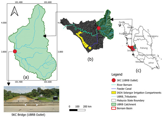
Figure 1.
Study area.
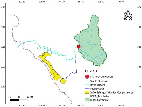
Figure 2.
Upper Bernam River Basin and IADA Selangor Irrigation Compartment.
2.2. Data Collection
- Climate Data: This study considered the climate simulations covering the historical period of 1985–2014 and the future period of 2020–2095. The CMIP6 data was collected from the Earth System Grid Federation (ESGF) data platform, while the Water Resources and Hydrology Division of Malaysia’s Department of Irrigation and Drainage (DID) provided the meteorological data.
- Hydrological Data: Data on average monthly streamflow [m3/s] in the vicinity of the study area’s outlet (Jambatan Kuala Slim (SKC) gauge station) for the years (1985–2022). These data were obtained from the Water Resources and Hydrology Division, Department of Irrigation and Drainage (DID), Malaysia.
- DEM (Figure 3a), Land Use Land Cover (Figure 3b), and Soil Data (Figure 3c): The Digital Elevation Model (DEM) was downloaded from the Shuttle Radar Topography Mission (SRTM) website and processed in QGIS. The DEM covered the catchment area and had a spatial precision of 30 m.
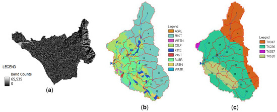 Figure 3. Spatial data inputs of the study area ((a): DEM, (b): Land-use map, and (c): Soil map).
Land use and land cover (LULC). The study area’s land use and the land cover map were obtained from the ESRI website (Global Land Cover; Sentinel-2: 10 m land use/land cover; the year 2022) and processed in QGIS 3.28.13 Firenze.
A digital soil map of the area was downloaded from the FAO Map Catalog (Digital Soil Map of the World (DSMW)-ESRI shapefile format) and processed in QGIS.
2.3. SWAT Model Setup
The Soil and Water Assessment Tool (SWAT) model was used to project climate change impacts on the streamflow of the Bernam watershed [15,16,17]. Therefore, evaluating the SWAT model before the projection was essential to know how the model behaves. The SWAT model is compatible with numerous computer programs. The QSWAT3_9 version 1.5.10 of the model, with an interface in QGIS 3.28.13 Firenze, was utilized for this study [18]. In addition, the SWAT Editor software [19] was employed for model calculations. The SWAT model is a deterministic model created by the United States Department of Agriculture [16,17,20]; it is applied to map physical, chemical, and biological processes using mathematical equations. It was developed to predict the effects of basin-scale management practices on water and agricultural chemical yields [16,17,21,22].
The SWAT Calibration and Uncertainty Programs (SWATCUP-premium) version [23] was used to calibrate and validate the SWAT model to the natural environment of the study area.
The SWATCUP is a calibration program for SWAT models. The program analyzes the SWAT model’s calibration, validation, sensitivity, and uncertainty [16,23,24]. The SUFI-2 algorithm was utilized because it is effective for small catchments [16,24,25,26].
Testing the SWAT model’s ability to predict how climate change affected the streamflow of the watershed, spatial data (DEM, LULC, and soil map) were obtained and input in the model setup. The “Edit Inputs and Run SWAT Model” window was populated with the following meteorological data for running the SWAT model: daily sums of precipitation [mm]; daily minimum and maximum air temperature [°C]; average daily wind speed [m/s]; daily mean relative humidity [%]; and daily sums of total solar radiation [MJ/m2].
2.4. Calibration and Validation of the SWAT-CUP
The SWAT model was calibrated in the SWATCUP premium program [15,16,17,27,28] to accurately represent the model in reality. This helped address the inadequacies and uncertainties exhibited by both the GCMs and SWAT output in the simulation of the hydrological processes of the study area. Data on average monthly flow velocities [m3/s] in the vicinity of the study area’s outlet for the years 1991–2000, 2001–2010, 2011–2020, 1991–2005, and 1991–2010 were used for this purpose because the trade-off of lengthier pre-processing and simulation periods does not necessarily equate to greater data quality, nor does higher-resolution data always result in improved performance [17].
Upon obtaining a suitable calibration result, the model was validated using monthly average flow velocities [m3/s] near the mouth (Jambatan Kuala Slim (SKC)) of the study area for the years 2001–2005; 2011–2015; 2021–2022; 2006–2015; and 2011–2020, respectively.
The best-fit parameter ranges were analyzed based on the accuracy requirements of calibration and validation outlined by [16,24,29,30,31,32,33], using the p-factor, r-factor, coefficient of determination (R2) (Equation (1)), Nash–Sutclif model efficiency coefficient (NSE) (Equation (2)), Percent Bias (PBIAS) (Equation (3)), Kling-Gupta Efficiency (KGE) (Equation (4)), and [16,30] for calibration, respectively.
where Q is a variable (e.g., discharge), and m and s stand for measured and simulated, and i is the i-th measured or simulated data.
where Q is a variable (e.g., discharge), m and s stand for measured and simulated, respectively, and the bar stands for average.
Q is a variable (e.g., discharge), and m and s are measured and simulated, respectively.
where , and , and r is the coefficient of linear regression between simulated and measured variables, and are means of simulated and measured data, and and are the standard deviations of simulated and observed data.
2.5. Climate Projection Scenarios
CMIP6 climate data for SSP126, SSP245, SSP370, and SSP585 (Table 1) were bias-corrected using a revised version (Figure 4) of the Climate-Smart Decision Support System (CSDSS) for downscaling hydro-meteorological variables [34,35]. The CSDSS was created in the Matrix Laboratory (MATLAB R2024b) environment using the statistical downscaling method “Delta Change Factor” [34]. This method has been widely utilized in hydrological modeling because it permits rapid application, direct scaling of scenarios to changes suggested by GCMs, and multi-models with results from different GCM scenarios [34,36,37]. For further details, see [13,34,38].

Table 1.
Outline details of the ten selected GCMs from CMIP6 GCMs.
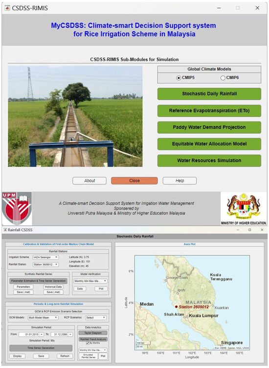
Figure 4.
Revised Climate-Smart DSS for downscaling climate variables for the CMIP5 and CMIP6 models.
The evaluated SWAT model was used to simulate and project the future impacts of climate change on streamflow. The projected changes in streamflow represent the relative variances from the reference period (1985–2020) for the five distinct 15-year periods in the future (2020s, 2040s, 2050s, 2070s, and 2080s).
3. Results
3.1. SWAT Model Calibration and Validation in UBRB
The uncalibrated runoff model exhibited suboptimal performance, evidenced by a Nash-Sutcliffe Efficiency (NSE) of −0.33 and a Pearson correlation value of 72%, as seen in Figure 5. Although the measured discharge is overestimated, the model demonstrates a substantial linear correlation (72%) between the predicted and observed flow. Before calibration, the model erroneously predicted runoff by overestimating the total water volume within the watershed. This necessitates calibration and validation of the model before future simulations of the hydrological processes.
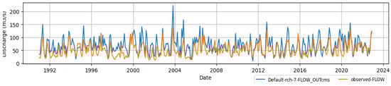
Figure 5.
Comparison between observed and simulated discharge at SKC gauge station, UBRB, for the calibration period 1991 to 2022.
Table 2 presents the iterations and performance indicator values for the calibrated and validated model output. The p-factor (0.82), r-factor (0.88), R2 (0.72), NSE (0.7), PBIAS (−1.1), and KGE (0.85) are the statistical extract of model performance during the calibration, while for the validation period, it has a p-factor (0.8), r-factor (1.04), R2 (0.75), NSE (0.65), PBIAS (−6.6), and KGE (0.79). However, a trade-off between the r-factor and p-factor exists because the r-factor can be increased to include more observations in the 95PPU; hence, it would improve the p-factor.
Table 2.
Overview of model performance indicators for performed iterations.
According to Abbaspour [39], the p-factor (≥0.7) and r-factor (≤1.5) assess the model calibration, with around 70% of observed data within the 95% PPU band (Figure 6). The calibration results meet Moriasi, Gitau [40], Moriasi, Arnold [41] criteria (NSE > 0.65; R2 > 0.5; |PBIAS| ≤ 25%), indicating a satisfactory model performance and effective simulation during calibration and validation.
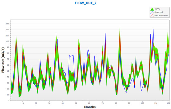
Figure 6.
The 95PPU plot of all variables for the calibrated model.
3.2. Projected Changes in Streamflow
The validated SWAT model was used to evaluate future changes in streamflow in the Upper Bernam River Basin. The assessment of climate change effects involved the combination of all simulations from the emission scenarios for the five future periods (2020s, 2040s, 2050s, 2070s, and 2080s). This study adopted the impact of climate variability with fixed land use in the future projections.
From the result, streamflow is projected to decline in the off seasons (January to June) in all future periods across all the SSP scenarios, with a transition in June–July. Nevertheless, changes in future flow compared to the historical period are most noticeable during the off-season period, with a mean decline of −15.9% under the SSP585 during the 2020s, as shown in Figure 7, Figure 8 and Figure 9. This phenomenon is anticipated because higher temperatures during the non-peak season typically lead to a greater rate of evapotranspiration than during the peak season, resulting in a subsequent change in future streamflow. In addition, the low (SSP126) and medium (SSP370) scenarios showed an average decline in streamflow of around −12.8% and −9.7%, respectively, for the same period (2020s, 2040s, 2050s, 2070s, and 2080s).
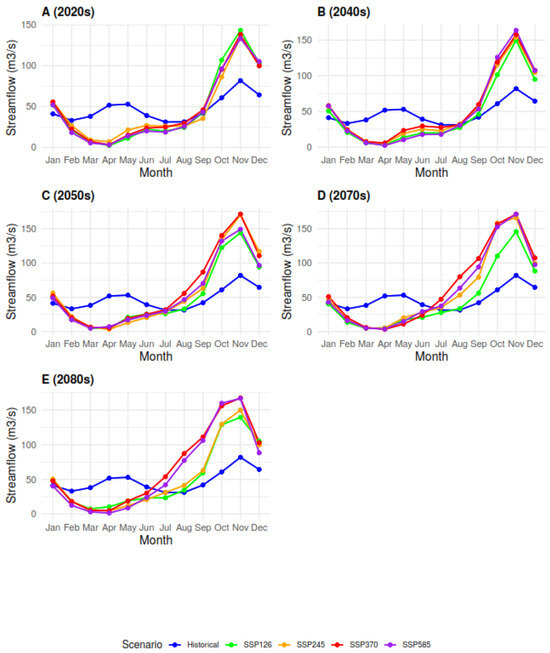
Figure 7.
Projected mean monthly streamflow under the different SSP scenarios and periods.
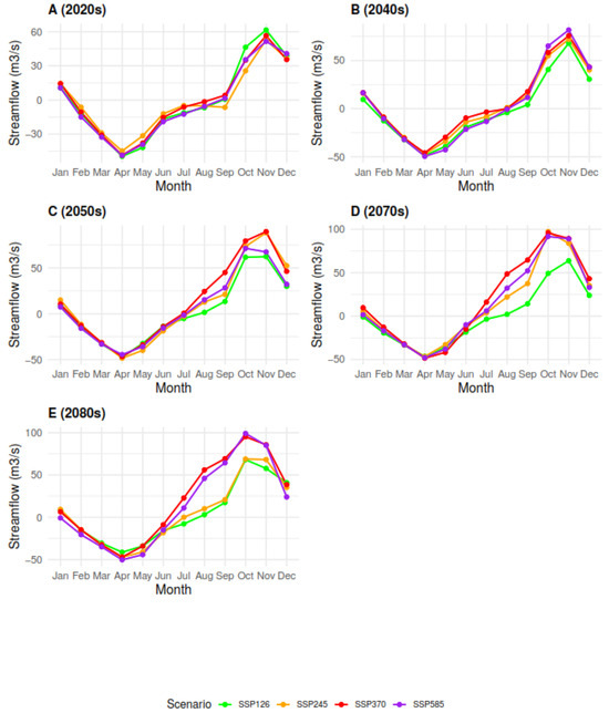
Figure 8.
Projected change of monthly streamflow under different SSP scenarios and periods.
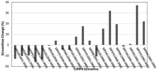
Figure 9.
Overall streamflow percent (%) change across various scenarios.
The result of the changes in the streamflow was observed to increase chronologically for the SSP scenarios except for SSP126. The increase in streamflow is projected to be higher for the SSP370 scenario than for the SSP585 scenario.
3.3. Seasonal Variation
The seasonal analysis with respect to the historical data revealed that the streamflow in the Upper Bernam River Basin shows seasonal variations under future climate scenarios. The off-season (January–June) streamflow declines, reaching −15.9% under SSP585, −12.8% under SSP126, and −9.7% under SSP370 during the 2020s, and this could be due to higher temperature and evapotranspiration [42,43]. The main-season (July–December) streamflow rises with peaks of 37.1% under SSP370 by the 2080s. This is driven by increased precipitation [13,44]. These findings highlight contrasting seasonal impacts of climate change on streamflow.
3.4. Monthly Streamflow Patterns
The monthly streamflow patterns decrease (Figure 7) in the off seasons from −13.4% to 0.7% during the 2020s–2040s and increase in the main seasons from 1% to 37.1% during the 2050s–2080s, with July marking a transition. The SSP370 scenario projects the highest increase (37.1%) in the 2080s, reflecting favorable wet-season runoff.
4. Discussion
The streamflow in the Upper Bernam River Basin (UBRB) is projected to experience contrasting trends between off seasons and main seasons under different Shared Socioeconomic Pathways (SSPs). During the off seasons of the 2020s, streamflow was projected to decline significantly, with the lowest mean flow of 18.82 m3/s observed under SSP585 and the highest of 24.55 m3/s under SSP245, compared to the historical mean of 42.73 m3/s. This represents a decrease ranging from 42.55% (SSP245) to 55.96% (SSP585). In contrast, during the main seasons of the same period, streamflow increased, ranging from 68.27 m3/s under SSP245 to 73.46 m3/s under SSP126, reflecting an increase of 31.52% to 42.55% from the historical mean of 51.91 m3/s.
In the 2040s, similar trends were observed. During the off seasons, mean streamflow ranged from 18.91 m3/s (SSP126) to 24.64 m3/s (SSP370), with declines of 55.73% and 42.34%, respectively. For the main seasons, flows ranged from 73.19 m3/s (SSP126) to 83.8 m3/s (SSP370), showing increases of 40.99% to 61.44%.
By the 2050s, off-season streamflow further declined, with SSP585 recording the lowest mean flow of 19.73 m3/s (53.83% decrease), and SSP370 the highest mean flow of 21.27 m3/s (50.21% decrease). Main-season flows increased significantly, ranging from 87.32 m3/s (SSP585) to 99.37 m3/s (SSP370), indicating increases of 68.22% to 91.44%.
Projections for the 2070s reveal the lowest off-season streamflow of 17.01 m3/s under SSP126 (60.2% decrease) and the highest of 20.17 m3/s under SSP245 (52.79% decrease). Main-season flows ranged from 76.82 m3/s (SSP126, 47.99% increase) to 111.5 m3/s (SSP370, 114.8% increase).
By the 2080s, the off-season streamflow reached its lowest point across all periods, with 15.09 m3/s observed under SSP585 (64.68% decrease), while SSP126 recorded the highest flow at 21.34 m3/s (50.07% decrease). Main-season flows peaked, ranging from 81.8 m3/s (SSP126, 57.6% increase) to 113.16 m3/s (SSP370, 118.01% increase).
Overall, the lowest off-season streamflow was observed in SSP585 during the 2080s, while the highest occurred in SSP370 during the 2040s. For the main seasons, the lowest flow was recorded in SSP245 during the 2020s and the highest in SSP370 during the 2080s. These findings indicate that SSP370 is associated with increased precipitation and peak flows, whereas SSP585 suggests reduced precipitation and lower streamflows.
The observed trends align with the findings of [38,45], who reported significant seasonal variations in streamflow for Malaysia’s Upper Bernam watershed. Their study, based on the 5th Assessment Report, also noted that precipitation during the main seasons is expected to increase across all scenarios compared to the off seasons.
This study shows the substantial seasonal and scenario-based variations in streamflow in the UBRB. The projections suggest that future hydrological patterns will be influenced strongly by the selected climate scenarios, with SSP370 yielding the highest increases in main-season flows and SSP585 the most pronounced declines during off seasons. These results emphasize the importance of integrating climate projections into water resource management plans to mitigate the impacts of extreme seasonal variations.
5. Conclusions
In this study, a simulation of the Upper Bernam River Basin’s streamflow was carried out using the SWAT model and CMIP6 data. The following are the key findings:
- The study area is characterized by mountainous terrain, with over 50% of the catchment covered by forest, 20.82% by oil palm, and 18.72% by rubber plantation. Despite the complex topography and diverse land cover, the model achieved high-performance metrics, including NSE, R2, and KGE, which were superior to those reported in similar studies. This highlights the robustness of the SWAT model in simulating hydrological processes for the Upper Bernam River Baasin.
- The streamflow projections showed a decline of −15.9% for SSP585 during the off-season of 2020s (January–June), while the flow increases by 37.1% for SSP370 during the main season of the 2080s (July–December), reflecting significant seasonal and long-term-climate change impacts.
- The seasonal variation in streamflow between the off seasons and main seasons calls for water resource conservation during peak flow periods to sustain agricultural and other uses in the UBRB.
6. Recommendation
Effective water management strategies should focus on mitigating the adverse impacts of reduced streamflow during the off-season and conserving increased main-season flows. Addressing the seasonal variability, policymakers should prioritize adaptive measures by enhancing water storage infrastructure and efficient allocation systems. Integrating climate-resilient practices into land-use planning and ecosystem conservation is essential to sustain hydrological balance in the UBRB under projected climate scenarios. Future studies should incorporate land use and soil changes to provide more comprehensive insights.
Author Contributions
Conceptualization, M.R.K. and M.D.Z.; methodology, M.R.K. and M.D.Z.; software, M.D.Z. and F.A.K.; validation, M.R.K., M.D.Z., M.S.F.B.M. and F.A.K.; formal analysis, M.R.K. and M.D.Z.; investigation, M.D.Z.; resources, M.R.K. and M.D.Z.; data curation, M.R.K.; writing—original draft preparation, M.D.Z.; writing—review and editing, M.R.K. and M.D.Z.; visualization, M.R.K. and M.D.Z.; supervision, M.R.K., N.M.R., B.M.R. and M.S.F.B.M.; project administration, M.R.K., N.M.R., B.M.R. and M.S.F.B.M.; funding acquisition, M.D.Z. All authors have read and agreed to the published version of the manuscript.
Funding
This research was funded by the Petroleum Technology Development Fund (PTDF), the Federal Republic of Nigeria, and the APC was funded by PTDF.
Data Availability Statement
Data are available upon request from the corresponding author due to Data were obtained from various government agencies, and some meteorological datasets were purchased under specific usage restrictions.
Acknowledgments
The authors acknowledge the financial support of Nigeria’s Petroleum Technology Development Fund (PTDF). Also, the financial support of the Putra Grant under Universiti Putra Malaysia (Grant No. 9769000) is gratefully acknowledged, and we appreciate the Department of Irrigation and Drainage (DID) and the Malaysian Meteorological Department (MMD) for providing the daily meteorological data for this study. Additionally, the authors acknowledge the support of the Soil and Water Engineering Research Group, Faculty of Engineering, University Putra Malaysia.
Conflicts of Interest
The authors declare no conflicts of interest.
References
- Mancosu, N.; Snyder, R.L.; Kyriakakis, G.; Spano, D. Water scarcity and future challenges for food production. Water 2015, 7, 975–992. [Google Scholar] [CrossRef]
- Porkka, M.; Gerten, D.; Schaphoff, S.; Siebert, S.; Kummu, M. Causes and trends of water scarcity in food production. Environ. Res. Lett. 2016, 11, 015001. [Google Scholar] [CrossRef]
- Roy, R. An introduction to water quality analysis. ESSENCE Int. J. Environ. Rehabil. Conserv. 2019, 9, 94–100. [Google Scholar] [CrossRef]
- Gheewala, S.H.; Silalertruksa, T.; Nilsalab, P.; Lecksiwilai, N.; Sawaengsak, W.; Mungkung, R.; Ganasut, J. Water stress index and its implication for agricultural land-use policy in Thailand. Int. J. Environ. Sci. Technol. 2018, 15, 833–846. [Google Scholar] [CrossRef]
- Cisneros, B.J.; Oki, T. Freshwater Resources. Climate Change 2014: Impacts, Adaptation, and Vulnerability. Part A: Global and Sectoral Aspects; Contribution of Working Group II to the Fifth Assessment Report of the Intergovernmental Panel on Climate Change; IPCC: Geneva, Switzerland, 2015; pp. 229–269. [Google Scholar]
- Li, M.; Xu, Y.; Fu, Q.; Singh, V.P.; Liu, D.; Li, T. Efficient irrigation water allocation and its impact on agricultural sustainability and water scarcity under uncertainty. J. Hydrol. 2020, 586, 124888. [Google Scholar] [CrossRef]
- Rahman, H.A. Global climate change and its effects on human habitat and environment in Malaysia. Malays. J. Environ. Manag. 2009, 10, 17–32. [Google Scholar]
- Hamed, M.M.; Nashwan, M.S.; Shahid, S. A novel selection method of CMIP6 GCMs for robust climate projection. Int. J. Climatol. 2022, 42, 4258–4272. [Google Scholar] [CrossRef]
- Kamal, A.M.; Hossain, F.; Shahid, S. Spatiotemporal changes in rainfall and droughts of Bangladesh for1. 5 and 2 °C temperature rise scenarios of CMIP6 models. Theor. Appl. Climatol. 2021, 146, 527–542. [Google Scholar] [CrossRef]
- Day, F. Energy-Smart Food for People and Climate; FAO: Rome, Italy, 2011. [Google Scholar]
- Malaysia, A.S. Strategies to Enhance Water Demand Management in Malaysia; Academy of Sciences Malaysia: Kuala Lumpur, Malaysia, 2016. [Google Scholar]
- Kondum, F.A.; Rowshon, M.K.; Luqman, C.A.; Hasfalina, C.M.; Zakari, M.D. Change analyses and prediction of land use and land cover changes in Bernam River Basin, Malaysia. Remote Sens. Appl. Soc. Environ. 2024, 36, 101281. [Google Scholar] [CrossRef]
- Dlamini, N.S.; Kamal, M.R.; Soom, M.A.B.M.; Faisal bin Mohd, M.S.; Abdullah, A.F.B.; Hin, L.S. Modeling potential impacts of climate change on streamflow using projections of the 5th assessment report for the Bernam River Basin, Malaysia. Water 2017, 9, 226. [Google Scholar] [CrossRef]
- Alansi, A.W.; Amin, M.S.M.; Abdul Halim, G.; Shafri, H.Z.M.; Aimrun, W. Validation of SWAT model for stream flow simulation and forecasting in Upper Bernam humid tropical river basin, Malaysia. Hydrol. Earth Syst. Sci. Discuss. 2009, 6, 7581–7609. [Google Scholar]
- Arnold, J.G.; Moriasi, D.N.; Gassman, P.W.; Abbaspour, K.C.; White, M.J.; Srinivasan, R.; Santhi, C.; Harmel, R.D.; Van Griensven, A.; Van Liew, M.W.; et al. SWAT: Model use, calibration, and validation. Trans. ASABE 2012, 55, 1491–1508. [Google Scholar] [CrossRef]
- Badora, D.; Wawer, R.; Nierobca, A.; Krol-Badziak, A.; Kozyra, J.; Jurga, B.; Nowocien, E. Modelling the hydrology of an upland catchment of Bystra River in 2050 climate using RCP 4.5 and RCP 8.5 emission scenario forecasts. Agriculture 2022, 12, 403. [Google Scholar] [CrossRef]
- Kmoch, A.; Moges, D.M.; Sepehrar, M.; Narasimhan, B.; Uuemaa, E. The Effect of Spatial Input Data Quality on the Performance of the SWAT Model. Water 2022, 14, 1988. [Google Scholar] [CrossRef]
- Dile, Y.T.; Daggupati, P.; George, C.; Srinivasan, R.; Arnold, J. Introducing a new open source GIS user interface for the SWAT model. Environ. Model. Softw. 2016, 85, 129–138. [Google Scholar] [CrossRef]
- Winchell, M.F.; Folle, S.; Meals, D.; Moore, J.; Srinivasan, R.; Howe, E.A. Using SWAT for sub-field identification of phosphorus critical source areas in a saturation excess runoff region. Hydrol. Sci. J. 2015, 60, 844–862. [Google Scholar] [CrossRef]
- Douglas-Mankin, K.; Srinivasan, R.; Arnold, J. Soil and Water Assessment Tool (SWAT) model: Current developments and applications. Trans. ASABE 2010, 53, 1423–1431. [Google Scholar] [CrossRef]
- Arnold, J.G.; Srinivasan, R.; Muttiah, R.S.; Williams, J.R. Large area hydrologic modeling and assessment part I: Model development 1. JAWRA J. Am. Water Resour. Assoc. 1998, 34, 73–89. [Google Scholar] [CrossRef]
- Smarzyńska, K.; Miatkowski, Z. Calibration and validation of SWAT model for estimating water balance and nitrogen losses in a small agricultural watershed in central Poland. J. Water Land Dev. 2016, 29, 31–47. [Google Scholar] [CrossRef]
- Abbaspour, K.C. SWAT Calibration and Uncertainty Programs. A User Manual; Swiss Federal Institute of Aquatic Science and Technology: Eawag, Switzerland, 2015; Volume 103, pp. 17–66. [Google Scholar]
- Abbaspour, K.; Vejdani, M.; Haghighat, S. SWAT-CUP Calibration and Uncertainty Programs for SWAT. Modsim 2007: International Congress on Modelling and Simulation: Land; Water and Environmental Management: Integrated Systems for Sustainability: Christchurch, New Zealand, 2007. [Google Scholar]
- Bilondi, M.P.; Abbaspour, K.C. Application of three different calibration-uncertainty analysis methods in a semi-distributed rainfall-runoff model application. Middle-East J. Sci. Res. 2013, 15, 1255–1263. [Google Scholar]
- Yang, W.; Andréasson, J.; Phil Graham, L.; Olsson, J.; Rosberg, J.; Wetterhall, F. Distribution-based scaling to improve usability of regional climate model projections for hydrological climate change impacts studies. Hydrol. Res. 2010, 41, 211–229. [Google Scholar] [CrossRef]
- Abbaspour, K.C.; Rouholahnejad, E.; Vaghefi, S.; Srinivasan, R.; Yang, H.; Kløve, B. A continental-scale hydrology and water quality model for Europe: Calibration and uncertainty of a high-resolution large-scale SWAT model. J. Hydrol. 2015, 524, 733–752. [Google Scholar] [CrossRef]
- Abbaspour, K.C.; Vaghefi, S.A.; Srinivasan, R. A guideline for successful calibration and uncertainty analysis for soil and water assessment: A review of papers from the 2016 international SWAT conference. Water 2017, 10, 6. [Google Scholar] [CrossRef]
- Abbaspour, K. SWAT-CUP Tutorial (2): Introduction to SWAT-CUP Program; Parameter Estimator (SPE); Swiss Federal Institute of Aquatic Science and Technology: Dübendorf, Switzerland, 2020. [Google Scholar]
- Houshmand Kouchi, D.; Esmaili, K.; Faridhosseini, A.; Sanaeinejad, S.H.; Khalili, D.; Abbaspour, K.C. Sensitivity of calibrated parameters and water resource estimates on different objective functions and optimization algorithms. Water 2017, 9, 384. [Google Scholar] [CrossRef]
- Abbaspour, K.C. User Manual for SWATCUP-2019/SWATCUP-Premium/SWATplusCUP Calibration and Uncertainty Analysis Programs; 2w2e Consulting GmbH Publication: Duebendorf, Switzerland, 2022. [Google Scholar]
- Chilkoti, V.; Bolisetti, T.; Balachandar, R. Multi-objective autocalibration of SWAT model for improved low flow performance for a small snowfed catchment. Hydrol. Sci. J. 2018, 63, 1482–1501. [Google Scholar] [CrossRef]
- Gupta, H.V.; Kling, H.; Yilmaz, K.K.; Martinez, G.F. Decomposition of the mean squared error and NSE performance criteria: Implications for improving hydrological modelling. J. Hydrol. 2009, 377, 80–91. [Google Scholar] [CrossRef]
- Ismail, H.; Kamal, M.R.; bin Abdullah, A.F.; bin Mohd, M.S.F. Climate-smart agro-hydrological model for a large scale rice irrigation scheme in Malaysia. Appl. Sci. 2020, 10, 3906. [Google Scholar] [CrossRef]
- Rowshon, M.K.; Dlamini, N.S.; Mojid, M.A.; Adib, M.N.M.; Amin, M.S.M.; Lai, S.H. Modeling climate-smart decision support system (CSDSS) for analyzing water demand of a large-scale rice irrigation scheme. Agric. Water Manag. 2019, 216, 138–152. [Google Scholar] [CrossRef]
- Abatzoglou, J.T.; Brown, T.J. A comparison of statistical downscaling methods suited for wildfire applications. Int. J. Climatol. 2012, 32, 772–780. [Google Scholar] [CrossRef]
- Fang, G.H.; Yang, J.; Chen, Y.N.; Zammit, C. Comparing bias correction methods in downscaling meteorological variables for a hydrologic impact study in an arid area in China. Hydrol. Earth Syst. Sci. 2015, 19, 2547–2559. [Google Scholar] [CrossRef]
- Dlamini, N.S. Decision Support System for Water Allocation in Rice Irrigation Scheme under Climate Change Scenarios; Universiti Putra Malaysia: Seri Kembangan, Malaysia, 2017. [Google Scholar]
- Abbaspour, K.C. The fallacy in the use of the “best-fit” solution in hydrologic modeling. Sci. Total Environ. 2022, 802, 149713. [Google Scholar] [CrossRef] [PubMed]
- Moriasi, D.N.; Gitau, M.W.; Pai, N.; Daggupati, P. Hydrologic and water quality models: Performance measures and evaluation criteria. Trans. ASABE 2015, 58, 1763–1785. [Google Scholar]
- Moriasi, D.N.; Arnold, J.G.; Van Liew, M.W.; Bingner, R.L.; Harmel, R.D.; Veith, T.L. Model evaluation guidelines for systematic quantification of accuracy in watershed simulations. Trans. ASABE 2007, 50, 885–900. [Google Scholar] [CrossRef]
- Arnell, N.; Reynard, N. The effects of climate change due to global warming on river flows in Great Britain. J. Hydrol. 1996, 183, 397–424. [Google Scholar] [CrossRef]
- Chien, H.; Yeh, P.J.-F.; Knouft, J.H. Modeling the potential impacts of climate change on streamflow in agricultural watersheds of the Midwestern United States. J. Hydrol. 2013, 491, 73–88. [Google Scholar] [CrossRef]
- Kabiri, R. Simulation of runoff using modified SCS-CN method using GIS system, case study: Klang watershed in Malaysia. Res. J. Environ. Sci. 2014, 8, 178. [Google Scholar] [CrossRef][Green Version]
- Ismail, H. Climate-Smart Agro-Hydrological Model for the Assessment of Future Adaptive Water Allocation for Tanjong Karang Rice Irrigation Scheme; Universiti Putra Malaysia, Universiti Putra Malaysia Institutional Repository: Serdang, Malaysia, 2020. [Google Scholar]
Disclaimer/Publisher’s Note: The statements, opinions and data contained in all publications are solely those of the individual author(s) and contributor(s) and not of MDPI and/or the editor(s). MDPI and/or the editor(s) disclaim responsibility for any injury to people or property resulting from any ideas, methods, instructions or products referred to in the content. |
© 2025 by the authors. Licensee MDPI, Basel, Switzerland. This article is an open access article distributed under the terms and conditions of the Creative Commons Attribution (CC BY) license (https://creativecommons.org/licenses/by/4.0/).