The Global 9 km Soil Moisture Estimation by Downscaling of European Space Agency Climate Change Initiative Data from 1978 to 2020

Abstract

The spatial resolution of current microwave remote sensing soil moisture (SM) data is about 25 km in global scale. The coarse scale hinders the application of SM product at regional scale. The global 9 km SM can be released by radar observations of Soil moisture Active and Passive (SMAP) satellite since 2015. For the failed radar sensor, SMAP 9 km SM is less than three months. Therefore, European Space Agency Climate Change Initiative (CCI) SM data is downscaled to 9 km using spatial temporal fusion model in the study. And the 43-year 9 km SM is downscaled by CCI data from 1978 to 2020. Results display that downscaled 9 km SM gets more detailed spatial information than CCI data. Moreover, temporal variation of CCI data in anomaly can be well captured by downscaled data. The evaluations against in-situ data indicate that temporal accuracies of downscaled data (r = 0.676, μbRMSE = 0.069 m³/m³) are comparable with CCI data (r = 0.670, μbRMSE = 0.070 m³/m³). Overall, downscaled data improves the spatial resolution of CCI data and inherits the temporal accuracy with slight improvement. Higher spatial resolution SM offers greater application potential. Additionally, the model herein enriches SM downscaling techniques.

1. Introduction

Soil moisture (SM) is one of the key factors in the climate system and is a basic element in the water cycle, energy cycle and the biogeochemical cycle [1,2,3]. It plays a crucial role in the hydrological and climate processes such as precipitation [4], runoff [5], evapotranspiration [6] and drought [7]. A variety of passive and active microwave satellites or sensors have been designed and launched since the 70s of last century for surface SM monitoring [8,9]. The global scale SM products, estimated from multiple microwave observation data, have been released with different resolution, different temporal span and different space coverage [10,11,12,13].

To solve the disunity of space and temporal in microwave SM, the European Space Agency has implemented the Climate Change Initiative (CCI) project since 2010. And then the long time series (from 1978 to now) SM products is estimated with 0.25° pixel size in global scale [14]. Nevertheless, the precise applications of CCI data is limited at regional scale for the coarse spatial resolution (~25 km), where the needed pixel size should be less than 10 km [15]. The 9 km SM, retrieved by SMAP (Soil Moisture Active and Passive) active and passive combined observations, is the first satellite based global scale SM with high spatial resolution and accuracy at the same time [16]. However, the failure of SMAP radar results in the available SMAP 9 km SM less than three months [17]. What is more noteworthy is that the global 9 km SM is absent before 2015. Hence, it has a negative impact on the long time series study of SM at regional scale. Therefore, it is worth studying how to downscale CCI data for the long time series global 9 km SM estimation.

The conventional SM downscaling methods can improve the spatial resolution of microwave SM from coarse scale to fine scale using the remotely sensed optical/thermal infrared (OTI) data [18,19,20,21,22,23,24,25]. Most studies focus on short-term or regional downscaling using OTI data. However, long-term global 9 km SM estimation without auxiliary datasets remains a challenge. In addition, the downscaling models depend on OTI data which is greatly polluted by cloud. Moreover, the relationship between microwave SM and OTI data cannot be well simulated by the downscaling model and it may bring much error to the downscaled fine scale SM [20,26]. Beyond that, conventional microwave SM downscaling approaches are further impacted by the scale effect. Therefore, the traditional approaches may impose considerable challenges on the estimation of 9 km SM data by CCI data downscaling.

The spatial temporal fusion model (STFM) can be used for fine scale SM estimation [27]. It presents a novel perspective to estimate global 9 km SM through CCI data. The use of the STFM model requires a pair of reference data with the same date including coarse scale and the corresponding fine scale data. Subsequently, the STFM is used to downscale microwave SM from coarse scale to fine scale at other date. Therefore, the STFM based downscaling of microwave SM merely necessitates SM data at diverse scales, without the requirement for supplementary auxiliary data (e.g., OTI data). With the assistance of historical SMAP 9 km and SMAP 36 km SM, STFM has been validated and can be used to estimate 9 km SM in global scale. It is also revealed that the estimated 9 km SM by STFM is better than the traditional downscaling method in spatial distribution, detailed information and the temporal accuracy [27]. Moreover, STFM has been widely used to estimate other surface parameters (e.g., Net Primary Productivity, Land surface temperature) with long time series and achieved good performance [28,29].

STFM is used to downscale CCI data for estimating 9 km SM in the study. The downscaled 9 km SM (DSM) has the same time series with CCI data. It is of great significance for us to understand the role of SM in atmospheric processes, and regional scientific researches and applications. This study integrates SMAP and CCI microwave data for estimating 9 km SM in global scale with long time series. It is convenient for practical production without the assistance of other satellite auxiliary data. Overall, the DSM, downscaled by STFM, can be considered to compensate for the lack of long time-series global 9 km SM products, particularly prior to 2015. The DSM is compared with the enhanced passive SMAP 9 km SM at the overlapping periods. Besides, the DSM is resampled to 0.25° and then compared with CCI data for the verification of time series consistency. The in-situ surface (less than 10 cm) SM data obtained from the International SM Network (ISMN) is used to evaluate the accuracy difference between DSM and CCI data. The contributions of this study are (1) Constructed the STFM based downscaling model integrating SMAP and CCI data; (2) Analyzed the spatial and temporal characteristic differences between DSM and CCI data; (3) Tested the accuracy of DSM against in-situ data. Generally, the model proposed in this study not only enriches downscaling techniques, but also the DSM data will greatly promote the researches and applications at regional scale.

2. Data

Based on the purpose of the study, SM products including the passive CCI data, SMAP data and ISMN in-situ data are used. The CCI data is downscaled to 9 km SM using STFM with the assistance of SMAP 9 km data. SMAP 36 km data and the enhanced SMAP 9 km data are used to evaluate the quality of DSM. ISMN in-situ data is used to evaluate the temporal accuracy of the pixel SM in terms of quantitative evaluation indicators.

2.1. SMAP Soil Moisture

SMAP 36 km data is retrieved from SMAP passive brightness temperature using the V-polarized single channel algorithm (SCA-V) [30]. SMAP 9 km data is retrieved by the same algorithm with SMAP 36 km data and the 9 km brightness temperature disaggregated from 36 km brightness temperature with the assistance of 3 km radar surface backscatter observed by SMAP radar. The disaggregation process ensures the consistency between disaggregated 9 km and 36 km brightness temperature, so SMAP 36 km and 9 km data are consistent in spatial distribution and temporal variation. As the error of disaggregated 9 km brightness temperature (2.73 K) is larger than the error of SMAP passive observation (1.3 K) resulting in the lower accuracy of SMAP 9 km SM. Nevertheless, the detailed spatial information of SMAP 9 km data can greatly strengthen our understanding of the coupling processes that link the terrestrial water, energy, and carbon cycles, improve the capability in flood prediction and drought monitoring, and enhance short-term weather and long-term climate forecasting skills. However, the failure of SMAP radar results in the available SMAP 9 km data less than three months (13 April–7 July 2015). To compensate for the adverse effects caused by the absent 9 km SM, the Backus-Gilbert interpolation method adopted by SMAP team is to post the passive microwave polarization brightness temperature onto 9 km and then the enhanced SMAP 9 km data is retrieved [17]. However, the lack of detailed spatial information still restricts the further applications of enhanced SMAP 9 km data.

2.2. CCI Soil Moisture

The passive CCI data is generated by merging multiple passive microwave SM products with different temporal span [9]. The whole period of CCI data used in the study can be divided into nine sub-periods (Table 1, sub_i, i = 1:9). The LPRM algorithm is used to retrieve the passive CCI data and then the retrieved SM is merged to construct the long time series passive 0.25° SM product. In the coincidence period of AMSR-E and other satellites, AMSR-E LPRM SM is treated as the benchmark. The microwave SM retrieved from other satellite is scaled to the range of AMSR-E product using a cumulative distribution function (CDF) [8]. There was no coincidence period prior to AMSR-E, it was assumed that the inter-annual temporal variation of SM in this segment is the same as that in AMSR-E, and then the SM is scaled to the range of AMSR-E product using CDF. After AMSR-E, the SMOS SM is retrieved by LPRM and then to integrate multi-source SM. Notably, only the observed data at night-time is used to retrieve CCI SM as the land surface temperatures at night-time are more homogeneous than at daytime, which is favorable for SM retrieval. Neglecting the differences in the transit time of the varied satellites, the time of CCI is set 0:00 UTC. The passive CCI SM data is downscaled to 9 km from 1978 to 2020 in the study.

Table 1. The passive CCI data merged by varied passive microwave data at varied periods.

Sensors	Time Period	Band(s)	Mark
SMMR	1 November 1978–31 July 1987	C	Sub_1
SSM/I	9 September 1987–31 December 1997	K	Sub_2
SSM/I, TMI, SSM/I	1 January 1998–18 June 2002	X, K	Sub_3
AMSR-E	19 June 2002–30 September 2007	C, X	Sub_4
AMSR-E, WindSat	1 October 2007–14 January 2010	C, X	Sub_5
AMSR-E, WindSat, SMOS	15 January 2010–4 October 2011	L, C, X	Sub_6
WindSat, SMOS	5 October 2011–30 June 2012	L, C, X	Sub_7
SMOS, AMSR2	1 July 2012–30 March 2015	L, C, X	Sub_8
SMOS, AMSR2, SMAP	31 March 2015–31 December 2020	L, C, X	Sub_9

2.3. In Situ Soil Moisture

ISMN in-situ data is used to evaluate the temporal accuracies of CCI and DSM in the study. The purpose of ISMN is to enable scientists to evaluate the accuracy of satellite based SM, test the reliability of algorithm, improve the retrieval algorithm, and finally get the microwave SM products with high accuracy [31]. There is a certain difference between the in-situ data and the satellite SM in the detection depth and spatial resolution [32]. Nevertheless, ISMN in-situ data has been widely used for SM evaluation focusing on America, European and Africa. Because it’s the field measurement, and it shows what the surface SM is really like. The depth of ground detection of passive microwave is affected by the frequency of observed band, thickness of vegetation canopy, SM and soil texture [33]. For the penetration capacity of microwave sensors, there are slight differences for diverse frequencies (e.g., 0–1/3 cm for X/C –band, and 0–5 cm for L-band) [34,35,36].

As the long time series (1978–2020) of the study, the appropriate in-situ data from ISMN should be selected to ensure the effectiveness of evaluations. Hence, the in-situ data that don’t meet the following arbitrary conditions are excluded: (1) the monitored surface soil depth should be less than 10 cm at first layer; (2) the valid in-situ time series of each site should be more than one year; (3) the temporal correlation between in-situ SM and the corresponding CCI pixel SM should be in positive and pass the hypothesis test (p-value is less than 0.05). The information of selected in-situ networks is shown in Table 2 and the spatial distribution of in-situ sites is shown in Figure 1.

Table 2. The selected in-situ data from ISMN (unit: m³/m³).

Network	NO.	Mean	Standard Deviation	Period	Country
AMMA	7	0.073	0.072	1 June 2006–31 December 2018	Benin, Niger, Mali
COSMOS	109	0.296	0.109	28 April 2008–29 March 2020	USA
CTP_SMTMN	17	0.210	0.114	1 August 2010–19 September 2016	China
HOAL	18	0.315	0.073	11 July 2013–31 December 2020	Austria
HOBE	30	0.204	0.069	8 September 2009–13 March 2019	Denmark
OZNET	31	0.129	0.081	12 September 2001–27 August 2018	Australia
PBO_H2O	110	0.125	0.080	27 September 2004–16 December 2017	USA
REMEDHUS	24	0.122	0.097	15 March 2005–31 December 2020	Spain
RSMN	16	0.147	0.064	9 April 2014–31 December 2020	Romania
SCAN	133	0.201	0.118	1 January 1996–31 December 2020	USA
SNOTEL	328	0.167	0.116	1 October 1980–31 December 2020	USA
SOILSCAPE	102	0.153	0.101	3 August 2011–29 March 2017	USA
USCRN	88	0.183	0.110	15 November 2000–31 December 2020	USA

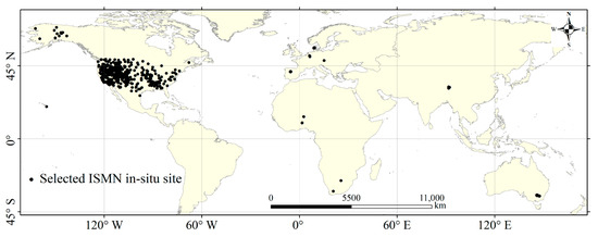
Figure 1. The spatial distribution of selected ISMN in-situ sites in the study.

3. Methods

The STFM, first proposed by Gao et al., (2006) [37], is designed to generate daily surface reflectance data with fine spatial resolution by integrating Landsat and MODIS data. Owing to its capability to efficiently synthesize spatial and temporal information from multi-scale datasets, the model has since been widely applied to other remote sensing domains, including SM monitoring, land surface temperature retrieval, and vegetation productivity estimation. In this study, it is employed to downscale CCI SM to a 9 km resolution.

In addition to SMAP data, other satellite auxiliary data (e.g., OTI data or radar data) are not used in the STFM for CCI downscaling. However, the 9 km SMAP data extension has only been implemented for two years, so the applicability of STFM to long-term soil moisture estimation remains unknown. Furthermore, in previous studies [37,38,39], the spatial distribution of reference data (paired coarse- and fine-scale data at the same time) used in STFM was highly similar. As we know, due to differences in observation methods and retrieval algorithms, the spatial distributions of CCI and SMAP SM differ significantly. Therefore, downscaling CCI data through fusion with SMAP data presents non-trivial challenges.

3.1. Soil Moisture Spatial Temporal Fusion Model

STFM assumes that SM has the same temporal variation parameters at different spatial resolutions. The model parameters of STFM are estimated at coarse scale and then are applied to fine scale. It can be considered that the temporal variation of coarse scale (C) SM is in linear equation (Equation (1)) from T₀ date to T_k date:

$$C\left(x,y,T_k\right)=a\left(x,y,\mathsf{\Delta }T\right)\times \overline{C\left(x,y,T_0\right)}+b\left(x,y,\mathsf{\Delta }T\right)$$

(1)

Meanwhile, the linear temporal variation at fine scale (F) is shown in Equation (2):

$$F\left(x,y,T_k\right)=a\left(x,y,\mathsf{\Delta }T\right)\times \overline{F\left(x,y,T_0\right)}+b\left(x,y,\mathsf{\Delta }T\right)$$

(2)

where $\overline{C\left(x,y,T_0\right)}$ and $\overline{F\left(x,y,T_0\right)}$ are the one or more paired reference data needed in STFM. $∆T=T_k-T_0$, $T_k$ is the date to be estimated and $T_0$ is the date of reference data. $a\left(x,y,∆T\right)$ and $b\left(x,y,∆T\right)$ are the linear regression coefficients estimated by Equation (1).

Moreover, SM has strong correlation in the spatial neighborhood information. Incorporating the spatial information of SM into Equations (1) and (2) can improve the estimation results. In general, the closer of the distance indicates the higher similarity of SM data. Hence, the neighborhood similar pixel information can be added into STFM making the more accurate estimation. The size of the neighborhood window dictates the complexity of the model. Typically, as the window expands, the computational complexity of the model increases, the estimation time lengthens noticeably, and the block effect in the estimated image becomes more prominent, accompanied by enhanced uniformity. Taking these factors into comprehensive consideration, the neighborhood window in this study is set to 5 × 5 for selecting similar pixels.

Please refer to Cheng et al. 2017 [38] for more details about similar pixels $(x_i,y_i)$ selection and the corresponding weight ($W$) calculation. With the aid of neighborhood similar pixels, a more accurate 9 km SM estimation model is presented as follows:

$$F\left(x,y,T_k\right)={\displaystyle \sum _{i=1}^{n}W\left(x_i,y_i,T_0\right)\times \left[a\left(x_i,y_i,\mathsf{\Delta }T\right)\times \overline{F\left(x,y,T_0\right)}+b\left(x_i,y_i,\mathsf{\Delta }T\right)\right]}$$

(3)

Because as we know, the STFM offers a simple and computationally efficient approach to soil moisture downscaling, as it relies only on multi-scale SM data without requiring auxiliary optical or thermal inputs [27]. It effectively preserves temporal consistency and is suitable for generating long-term global products. However, its main limitation lies in the assumption of linear temporal variation across scales [37,38], which restricts its ability to capture complex nonlinear spatial–temporal relationships driven by vegetation, soil texture, and climate variability.

3.2. CCI Data Downscaling for 9 km SM Estimation Using STFM

To estimate DSM by CCI downscaling, the paired reference data of STFM should contain 9 km SM and CCI data at same date. The SMAP 9 km SM is taken as the fine scale data in STFM in the study. Due to the 2–3 day revisit period of SMAP satellite, there is a significant difference in spatial coverage between daily SMAP 9 km SM and CCI data. To improve the efficiency of CCI downscaling, the reference data of STFM should have as much spatial coverage as possible. Therefore, composition of multi-day data can construct the reference data of STFM that meets the requirements. It is reported that SMAP 36 km SM can be downscaled to 9 km by STFM with one paired reference data which is constructed by the 8-day composed historical SMAP 36 km SM and SMAP 9 km SM [27]. It provides the theoretical foundation for global long time series 9 km SM estimation by CCI downscaling in the study.

Given the long period of the study, all available SMAP 9 km data (three months, 13 April–7 July 2015) are used in constructing the reference dataset to ensure the accuracy of the estimation results. Thus, the averaged three months SMAP 9 km data and the CCI data at the same date are used to compose one paired reference data of STFM. The composed SM is shown in Figure 2. The time difference between CCI and SMAP data is neglected. Notably, the pixel size of SM at different scale should be same in STFM. Hence, the CCI data is resampled to 9 km size (equal-area scalable Earth 2.0, EASE2.0) before calculation in the study.

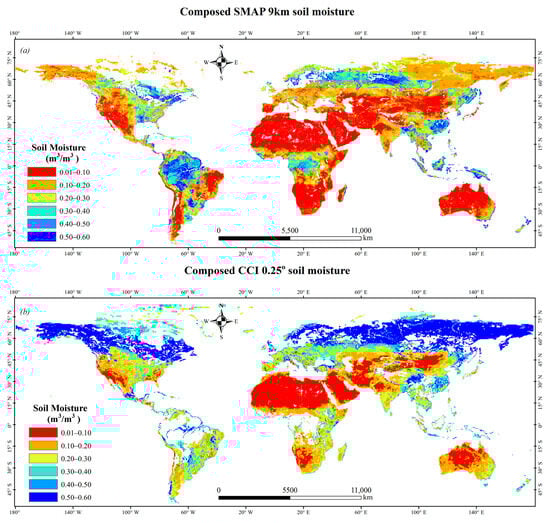
Figure 2. The composed reference SM: (a) SMAP 9 km data, (b) CCI data.

The flowchart of daily DSM data estimation is shown in Figure 3. The composed CCI (Figure 2b) and the daily CCI are used to configure the STFM and then to calculate the linear regression coefficients and the weight of similar pixels. Next, the composed SMAP 9 km data (Figure 2a) is coupled with the calculated STFM parameters for the daily DSM data estimation. In this way, the daily downscaling of CCI data has been completed. Finally, repeat the processes in sequence until all daily CCI data are downscaled to 9 km by STFM and the 43-year (1978–2020) DSM data is estimated in the study.

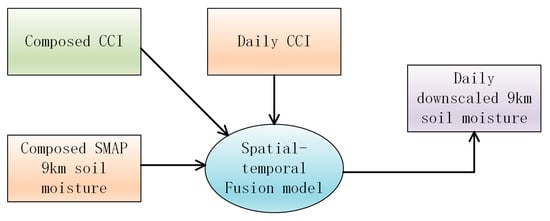
Figure 3. CCI downscaling for daily DSM estimation by STFM.

3.3. Evaluation Indictors of Downscaled 9 km SM

The qualitative and quantitative manners are combined for DSM data evaluations in terms of spatial distribution, detailed spatial information, temporal variation and temporal accuracy. The DSM is evaluated for the spatial distribution and detailed information by visual in qualitative. And then, it is evaluated by average gradient ($\overline{\mathit{g}}$, Equation (4)) in quantitative, which is to evaluate the richness of detailed spatial information.

$$\overline{\mathit{g}}={\displaystyle \frac{{\displaystyle \sum _{\mathit{i}}^{\mathit{M}-1}{\displaystyle \sum _{\mathit{j}}^{\mathit{N}-1}\sqrt{\frac{{\left(\mathit{S}\mathit{M}\left(\mathit{i},\mathit{j}\right)-\mathit{S}\mathit{M}(\mathit{i}+1,\mathit{j})\right)}^2+{\left(\mathit{S}\mathit{M}\left(\mathit{i},\mathit{j}\right)-\mathit{S}\mathit{M}(\mathit{i},\mathit{j}+1)\right)}^2}{2}}}}}{\left(\mathit{M}-1\right)\left(\mathit{N}-1\right)}}$$

(4)

where $\left(\mathit{i},\mathit{j}\right)$ indicates the pixel location of SM. $\mathit{M}$ and $\mathit{N}$ indicate the rows and columns of SM. The greater $\overline{\mathit{g}}$ indicates the more abundant detailed spatial information. The detailed spatial information will be benefit for the applications in high spatial heterogeneity areas.

Referencing previous research [40], DSM data (aggregated to 0.25°) is compared with CCI data to explore temporal variation discrepancies. The in-situ data from ISMN is used to evaluate the temporal accuracies of CCI and DSM data with the quantitative indicators including the correlation coefficient (r), bias (in-situ/aggregation—CCI), root mean square error (RMSE), and the unbiased RMSE ($\mu bRMSE=\sqrt{{RMSE}^2-{bias}^2}$). Notably, the pixel size of CCI data is resampled to 9 km (EASA2.0) before the temporal accuracy evaluation by ISMN in-situ data. The daily averaged in-situ SM is used as the reference to evaluate the 9 km SM. Generally, if there is one or more in-situ sites in the 9 km pixel footprint, data of the one in-situ site or the spatially-averaged value of multiple in-situ sites are used for evaluation.

In addition, the temporal variation of SM in anomaly is calculated for the revealing extreme weather events (e.g., precipitation and drought events) as the periodic variation of SM. It is extracted by the 35-day temporal windows [41] subtracting the periodic temporal variation of SM in the study. As many missing data in the temporal variation of CCI data, the extraction of SM in anomaly cannot guarantee the availability of all data in the 35-day moving window. Hence, to extract the SM in anomaly, the following two conditions should be met. First, the total valid data points must be at least 7 in the 35-day moving window. Second, each 17-day moving window (both before and after the SM) must contain at least 3 valid data points.

4. Results

The 43-year (1978–2020) DSM is shared to PANGAEA and available for free download at https://doi.pangaea.de/10.1594/PANGAEA.940409 websit (accessed on 23 July 2022). It contains 15,402 images, one image per day, with a total data volume of 13.6 G. The data is in integer format and the valid range is from 1 to 10,000, null or invalid values are represented by 0. To obtain the true SM in volumetric (m³/m³), the dataset should be multiplied by 0.0001.

4.1. The Spatial Distribution of Downscaled 9 km Soil Moisture

Figure 4 shows the spatial distribution of 8-day averaged (1–8 August 2020) DSM, enhanced SMAP 9 km SM, SMAP 36 km SM and CCI SM. The spatial coverage of DSM is less than CCI. As the temporal variation parameters of STFM are calculated by the paired reference data and daily CCI data, 9 km SM is estimated only in areas with the existed two data simultaneously. Meanwhile, the CCI and SMAP data are not spatio-temporal seamless and there is a phenomenon of inconsistent positions of void data. The spatial coverage of the intersection between CCI and SMAP data should be smaller than the spatial coverage of any data. Therefore, it suggests that the spatial coverage of daily DSM is not greater than the corresponding reference data and the daily CCI data.

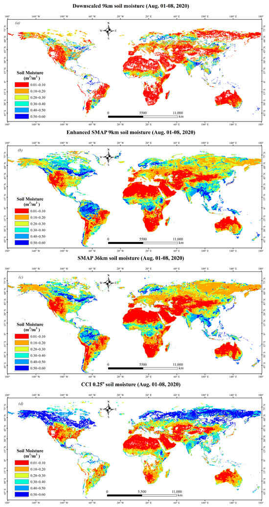
Figure 4. The spatial distribution of 8-day (1–8 August 2020) averaged SM: (a) DSM, (b) enhanced SMAP 9 km SM, (c) SMAP 36 km SM and (d) CCI SM.

The spatial distribution of DSM and CCI data is quite different, however, the difference between DSM and SMAP SM is relatively small (Figure 4). It mainly because that the temporal variation parameters of STFM are calculated by the daily CCI and composed CCI in reference data (Figure 2b) and then the parameters are applied to the composed SMAP 9 km SM in reference data (Figure 2a) for DSM estimation. Essentially, there is a linear relationship between DSM and the composed SMAP 9 km SM in reference data without considering the influence of similar pixels. Therefore, it can be regarded that the spatial distribution of DSM should be consistent with SMAP SM.

The spatial difference between the 8-day (1–8 August 2020) averaged SM (Figure 5) shows that CCI and SMAP SM are more or less greater than DSM in numerical across most areas of the world. The difference between CCI and DSM is larger than 0.2 m³/m³ at many regions of the world, especially at the high latitude areas (Figure 5a). This phenomenon does not appear in Figure 5b and most of the differences between DSM and SMAP SM fluctuate within 0.2 m³/m³. Due to the consistency of the spatial distribution of SMAP SM products [42,43], it can be confirmed that the spatial distribution of DSM is inherited by SMAP SM.

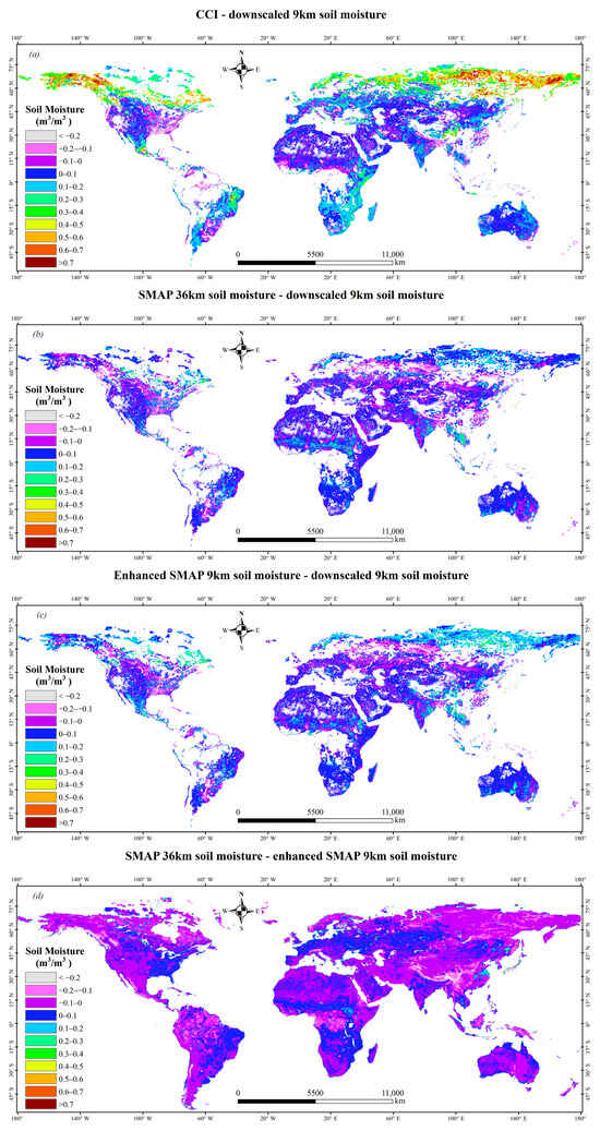
Figure 5. The difference between the 8-day (1–8 August 2020) averaged SM: (a) CCI—DSM, (b) SMAP 36 km SM—DSM, (c) enhanced SMAP 9 km SM—DSM and (d) SMAP 36 km SM—enhanced SMAP 9 km SM. Both CCI and SMAP 36 km SM are resampled to 9 km using the bilinear interpolation method.

4.2. The Detailed Spatial Information of Downscaled 9 km Soil Moisture

The detailed spatial information of 8-day (1–8 August 2020) averaged SM under the varied vegetation density is shown in Figure 6. The $\overline{\mathit{g}}$ is used as the quantitative evaluation index for characterizing the richness of detailed spatial information (Table 3). Notably, the data contains richer spatial details, which should enhance its adaptability in characterizing heterogeneous regions.

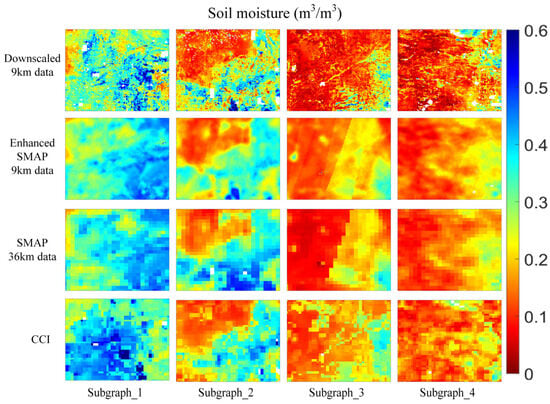
Figure 6. The detailed spatial information of SM under varied vegetation density.

Table 3. The average gradient ($\overline{\mathit{g}}$) of subgraphs shown in Figure 6.

	Subgraph_1	Subgraph_2	Subgraph_3	Subgraph_4
DSM	0.0537	0.0489	0.0417	0.0432
enhanced SMAP 9 km SM	0.0094	0.0099	0.0059	0.0060
SMAP 36 km SM	0.0088	0.0104	0.0054	0.0050
CCI	0.0169	0.0137	0.0128	0.0123

Note: SMAP 36 km SM and CCI data are resampled to 9 km using the bilinear interpolation method.

DSM significantly enhances the spatial resolution and enriches the detailed information of CCI data. It shows that the heterogeneity of surface feature is more clearly in DSM (Figure 6). In the subgraph of the third column, there is a linear surface feature in the middle of DSM, but CCI and SMAP SM cannot show the surface feature very well. In the subgraph of the fourth column, there is a clear linear object in DSM, while the linear features in the CCI and SMAP SM are not very clear. It suggests that the DSM has more abundant spatial information and may be beneficial to improve the application scopes of CCI data.

The $\overline{\mathit{g}}$ of DSM is greater than CCI obviously and the $\overline{\mathit{g}}$ increases about twice from CCI data with 0.25° to DSM data with 9 km for each subgraph (Table 3). The $\overline{\mathit{g}}$ of SMAP 36 km SM is less than CCI as the spatial resolution of CCI data is slightly greater than SMAP 36 km SM. The interpolation ratio to 9 km for CCI data (~25 km/9 km = 2.8) is less than for SMAP 36 km SM (36 km/9 km = 4). The $\overline{\mathit{g}}$ of SMAP 36 km SM and enhanced SMAP 9 km SM are comparable, because enhanced SMAP 9 km SM is retrieved by Backus-Gilbert interpolated passive SMAP brightness temperature. In essence, the SMAP 36 km SM and enhanced SMAP 9 km SM are derived from the same earth observation data with different calculation processes. Hence, it suggests that the spatial interpolation of CCI data can maintain the detailed spatial information of 9 km SM better than SMAP data. Overall, DSM gets the best $\overline{\mathit{g}}$ among the pixel SM indicating the more abundant spatial information for study at heterogeneous regions.

4.3. The Temporal Variation of Downscaled 9 km Soil Moisture Against CCI Data

Although DSM is the SMAP-like 9 km SM in spatial distribution, it is estimated by CCI downscaling using STFM from 1978 to 2020. Whether DSM can maintain the characteristics of CCI data in temporal variation remains to be further confirmed. Moreover, the temporal variation of SM plays an indispensable role in practical applications such as flood prediction, drought warning and world climate change [44]. To investigate the temporal variation difference, the DSM is aggregated to 0.25° maintaining the same pixel size as CCI data. The temporal r and RMSE are calculated between aggregated DSM (0.25°) and CCI SM at pixel scale globally.

It can be seen that the areas with temporal r lower than 0.9 are mainly concentrated in the high latitude, high vegetation coverage and arid regions (Figure 7). Nevertheless, the global mean temporal r in the whole period (1978–2020) is very high and larger than 0.97 (Table 4). In terms of temporal RMSE, the spatial distribution is similar with the temporal r. It shows that the high temporal r is consistent with the low temporal RMSE. The global mean temporal RMSE is very high for whole period and each sub-period of CCI data. Except the sub_2 and sub_7 periods, the temporal RMSE of other periods is not less than 0.1 m³/m³ (Table 4). Therefore, it can be considered that the temporal variation of CCI can be well captured by DSM because of the high mean temporal r. Meanwhile, the high temporal RMSE agrees with the results shown in Figure 5 indicating the large uncertainty between DSM and CCI data in temporal variation. Nevertheless, it will not affect the applications that need the high resolution SM focusing on the relative temporal variation of SM.

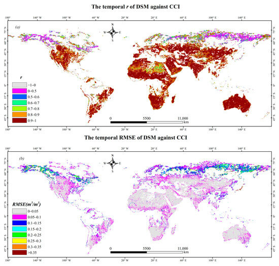
Figure 7. The temporal r (a) and RMSE (b) between aggregated DSM (0.25°) and CCI data.

Table 4. Global mean of temporal r and RMSE between aggregated DSM (0.25°) and CCI data.

	Sub_1	Sub_2	Sub_3	Sub_4	Sub_5	Sub_6	Sub_7	Sub_8	Sub_9	Whole
r	0.941	0.961	0.976	0.985	0.986	0.982	0.982	0.978	0.976	0.973
RMSE (m3/m3)	0.145	0.099	0.101	0.114	0.109	0.126	0.094	0.132	0.150	0.130

Spatial distribution of the temporal r in anomaly is shown in Figure 8. The temporal r of anomaly remains very high; meanwhile, it is lower than that of the original across most parts of the world (Figure 8b). It shows that the seasonal variation of SM has promoted the temporal r in original. It is consistent with the previous studies [45,46]. With the removal of seasonal factors, the global mean of temporal r in anomaly for DSM is 0.948, slightly less than the temporal r in original shown in Table 4. The results show that DSM can well capture the temporal variation of CCI data in anomaly (e.g., precipitation and drought events). It further confirms the ability of DSM to capture CCI data, suggesting that DSM can reveal the global climate change of CCI data at finer scale.

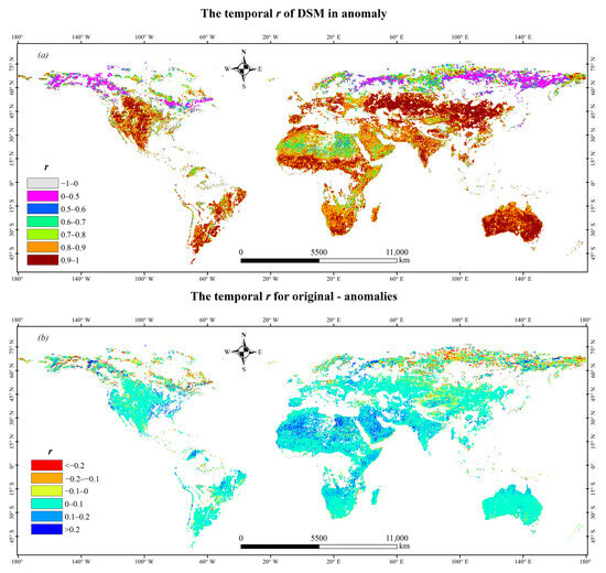
Figure 8. Temporal r of DSM in anomaly (a) and the difference of temporal r (b).

4.4. Evaluation of Downscaled 9 km Soil Moisture Against ISMN In Situ Data

The temporal variations of DSM, CCI, enhanced SMAP 9 km SM and in-situ SM are shown in Figure 9 in case of Oznet and REMEDHUS SM monitoring network from 1 January 2016 to 31 December 2017. Note that all the valid pixel SM and in-situ SM over Oznet and REMEDHUS are arithmetically averaged. It can be obviously seen that the three types of pixel scale SM data can well capture the temporal variation of in-situ measurements in OZNET and REMEDHUS. CCI and DSM exhibit similar temporal volatility and both overestimate in-situ measurements across the two monitoring networks. Enhanced SMAP 9 km SM is closer to in-situ data than DSM and CCI in numeric. Meanwhile, the enhanced SMAP 9 km SM is numerically closer to the in-situ measurements compared to the other two datasets. Nevertheless, due to its 2–3-day revisit cycle, the enhanced SMAP 9 km SM is significantly inferior to the daily CCI and CAP datasets in terms of temporal continuity.

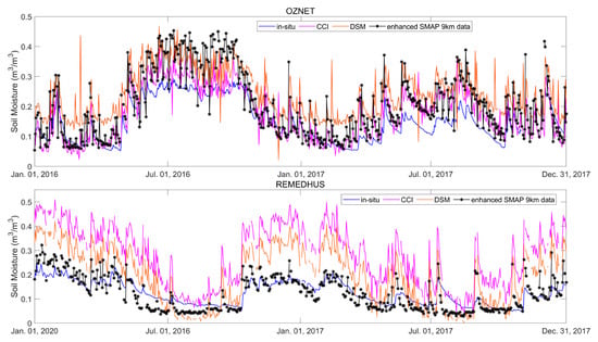
Figure 9. Temporal variation of SM from 1 January 2016 to 31 December 2017 at Oznet and REMEDHUS.

There is a certain mismatch between ISMN in-situ sites and pixel SM in spatial resolution, observation time and detection depth. The reliability of the temporal variation evaluation results is disputed by previous works in a single spare site [43,47,48,49]. Therefore, this study only calculates the arithmetically averaged evaluation results of the ISMN monitoring networks. Prior to the launch of the SMAP satellite in 2015, the global spatial resolution of SM was approximately 25 km, and 9 km global SM data remained unavailable. Based on the acquisition time of SMAP SM data, the study divides the evaluation against ISMN in-situ data into two phases: pre-SMAP and post-SMAP. This two-period division is more appropriate for assessing the temporal accuracy of 9 km pixel scale SM. To enhance the comparability of evaluation results between the two phases, the in-situ monitoring networks selected from ISMN are kept consistent across both periods.

As most ISMN monitoring stations operate normally after 2000, the evaluations based on ISMN in-situ data began in 2000 in this study. Table 5 shows the evaluations against ISMN SM from 1 January 2000 to 12 April 2015 (pre-SMAP). The best value for each index is in bold. The temporal accuracy of CCI SM varies significantly among different ISMN monitoring networks. It is consistent with the previous studies and gets the similar evaluation results [50,51,52]. Generally, it can be seen that the temporal accuracies of DSM are very close to CCI. It suggests that the temporal accuracy of DSM inherits from CCI. For bias and RMSE, there is no clear directionality in the performance of DSM and CCI at different in-situ networks. Nevertheless, the temporal r and μbRMSE of DSM are slight better than CCI at most monitoring networks (Bold font in Table 5). Moreover, the average accuracy of DSM (r = 0.592, bias = −0.029 m³/m³, RMSE = 0.108 m³/m³ and μbRMSE = 0.066 m³/m³) performs slight better than CCI. It is mainly because that the spatial and temporal information are taken into consideration for 9 km SM estimation weakening the outlier information of CCI data.

Table 5. The evaluations of DSM against ISMN in-situ SM from 1 January 2000 to 12 April 2015 (bias means in-situ SM—pixel SM). Bold numbers are necessary to highlight significant differences in this article.

Network	r		bias (m3/m3)		RMSE (m3/m3)		μbRMSE (m3/m3)
	CCI	DSM	CCI	DSM	CCI	DSM	CCI	DSM
AMMA	0.640	0.656	−0.028	−0.012	0.059	0.056	0.046	0.045
COSMOS	0.465	0.474	0.003	−0.015	0.125	0.148	0.073	0.073
CTP_SMTMN	0.599	0.604	−0.103	−0.062	0.130	0.126	0.061	0.061
HOAL	0.606	0.606	−0.132	0.014	0.152	0.083	0.074	0.074
HOBE	0.634	0.640	−0.145	−0.046	0.153	0.079	0.046	0.043
OZNET	0.647	0.658	−0.038	−0.096	0.083	0.137	0.060	0.058
PBO_H2O	0.632	0.646	−0.033	0.011	0.083	0.078	0.058	0.056
REMEDHUS	0.679	0.682	−0.167	−0.080	0.193	0.139	0.089	0.088
SCAN	0.464	0.484	−0.034	−0.032	0.102	0.115	0.074	0.072
SNOTEL	0.410	0.429	−0.029	−0.022	0.125	0.125	0.090	0.087
SOILSCAPE	0.672	0.683	0.021	0.040	0.083	0.087	0.061	0.060
USCRN	0.535	0.545	-0.041	-0.049	0.116	0.122	0.072	0.069
Average	0.582	0.592	-0.061	-0.029	0.117	0.108	0.067	0.066

Table 6 shows the evaluations against ISMN SM from 13 April 2015 to 31 December 2020 (post-SMAP). Unlike Table 5, Table 6 is not limited to comparing the accuracy discrepancies between DSM and CCI. It further extends the comparison to the AMSR2 SM retrieved by LPRM algorithm [53,54] and the enhanced SMAP 9 km SM. Notably, since AMSR2 has no inherent correlation with DSM, conducting an accuracy difference analysis between them can better demonstrate the performance of DSM. Compared with Table 5, the average accuracies of CCI and DSM have improved during the period. The possible main reason is that the CCI data in Table 5 is obtained by fusing observation data from multiple different time periods (Table 1), and the errors between the data are not fully coordinated. Similar to Table 5, the temporal accuracy of DSM in Table 6 is still slightly better than CCI. The average accuracy of DSM (r = 0.676, μbRMSE = 0.069 m³/m³) is slightly lower than enhanced SMAP 9 km SM (r = 0.695, μbRMSE = 0.057 m³/m³) and better than AMSR2 (r = 0.615, μbRMSE = 0.079 m³/m³). The accuracy of DSM is not yet comparable to that of SMAP data, but this accuracy is also slightly improved compared to CCI. More importantly, the time series of DSM is same as CCI data. The compromise between accuracy and long time series may give DSM an advantage in climate data research.

Table 6. The evaluations of DSM against ISMN in-situ SM from 13 April 2015 to 31 December 2020.

Network	r				μbRMSE (m3/m3)
	CCI	DSM	Enhanced SMAP 9 km SM	AMSR2	CCI	DSM	Enhanced SMAP 9 km SM	AMSR2
AMMA	0.821	0.831	0.834	0.645	0.033	0.032	0.042	0.045
COSMOS	0.518	0.510	0.561	0.427	0.079	0.079	0.058	0.106
CTP_SMTMN	0.770	0.772	0.793	0.866	0.055	0.054	0.071	0.029
HOAL	0.635	0.629	0.630	0.537	0.126	0.123	0.054	0.150
HOBE	0.693	0.699	0.703	0.459	0.046	0.045	0.054	0.079
OZNET	0.755	0.757	0.766	0.835	0.063	0.062	0.071	0.059
PBO_H2O	0.714	0.726	0.750	0.632	0.055	0.053	0.048	0.062
REMEDHUS	0.706	0.708	0.695	0.841	0.085	0.084	0.053	0.050
SCAN	0.553	0.565	0.611	0.535	0.080	0.078	0.056	0.088
SNOTEL	0.525	0.542	0.539	0.391	0.085	0.083	0.076	0.106
SOILSCAPE	0.727	0.733	0.771	0.720	0.053	0.052	0.054	0.063
USCRN	0.629	0.639	0.687	0.578	0.080	0.078	0.052	0.091
Average	0.670	0.676	0.695	0.615	0.070	0.069	0.057	0.079

Overall, DSM can provide abundant spatial detailed information in fine scale for the future applications and studies with the temporal accuracy no less than CCI data. Meanwhile, DSM can be taken as the SMAP-like SM in spatial distribution, but the temporal accuracy is less than SMAP SM (The target μbRMSE < 0.04 m³/m³). Nevertheless, it can be considered that DSM is the extension of SMAP SM before 2015. Therefore, CCI downscaling using STFM and SMAP 9 km SM data can acquire the SMAP-like long time series 9 km SM providing the choice for studies and applications at regional scale.

5. Discussions

The above results have well demonstrated the spatial distribution characteristics, temporal variation features, and accuracy of the DSM. However, aspects such as the limitations of the DSM, its attribution characteristics, comparative analysis with traditional methods, and data accuracy prior to 2000 require further discussion and analysis.

5.1. Analysis of the Difference Between DSM and CCI

DSM data may be considered a derivative of CCI data. As the error sources and distribution of CCI data have been thoroughly addressed in prior studies [9,14,52], analyzing the discrepancies between DSM and CCI enables a comprehensive understanding of the error characteristics of DSM. On this basis, the daily r and RMSE between DSM and CCI are computed (Figure 10). The daily r is general less than 0.9 and daily RMSE is larger than 0.1 m³/m³ obviously. The moderate high correlation and relatively high RMSE indicate the inadequate consistency between CCI and DSM. In addition, the daily r and RMSE show a large fluctuation with temporal variation. The volatility is the smallest in the Sub_3 period (Table 1), the largest in the first two periods, and falls between these two extremes in the other periods. Meanwhile, the change trends are similar in the two consecutive red dotted lines (sub-period division of CCI data, Table 1), but the difference is very obvious between the red dotted lines. The phenomenon may be caused by the multi-source data integration of CCI data [51] and the time distance between estimation date and reference date of STFM [27,37,38].

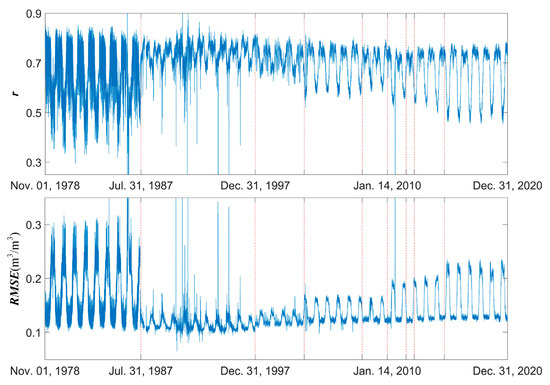
Figure 10. The daily r and RMSE of aggregated DSM against CCI. The red dotted line is the sub-divisions of CCI data shown in Table 1.

The different microwave observations are used to generate CCI data at different sub-period. Although the benchmark algorithm of SM retrieval is LPRM for the varied passive microwave observations, the internal differences of varied microwave observation band (e.g., L band, C band and X band) cannot be eliminated by the benchmark algorithm [51,55]. Hence, the significant differences in daily r and RMSE between different sub-periods of CCI cannot be avoided. The internal difference is very similar in the same sub-period for daily r and RMSE. The seasonal variation of SM may be the main cause of this phenomenon.

In addition, the time distance between estimation date and reference date may be the other factor. In the principle of STFM, the longer time distance, the greater uncertainty of finer scale data estimation [37,38]. Shown in Figure 10, the high-value and low-value regions in the Sub_1 period exhibit no significant discrepancy from those in the reference period (13 April–7 July 2015) of STFM; furthermore, the high-value region in the Sub_1 period is slightly larger than that in the reference period. It suggests that the effect of time distance on STFM downscaling is not significant as the relatively stable daily r and RMSE. It can be considered that the STFM can be used for long time series DSM estimation in global scale. More importantly, both 9 km and 25 km are very large scales: a single pixel covers over 80 square kilometers, and even subtle surface changes within such a pixel are barely detectable at the 9 km scale. This is precisely what enables the robust performance of 9 km soil moisture estimation in this study. Nevertheless, it is important to note that without high-spatial-resolution data, STFM cannot directly estimate the corresponding high-spatial-resolution data using low-resolution data alone.

5.2. Analysis of the Similarity Between DSM and SMAP

Although the DSM is derived from the downscaling of CCI data, it can be regarded as SMAP-like data based on Figure 4 and the principle of SFTM. Notably, the attribution does not take into account the numerical differences among CCI, SMAP and DSM completely. Therefore, the quantitative evaluations of DSM and CCI against SMAP 36 km data is investigated (Figure 11).

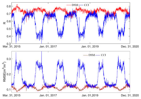
Figure 11. The daily r and RMSE of DSM and CCI against SMAP 36 km SM.

There are obvious seasonal fluctuations in the daily r and RMSE of DSM compared with SMAP 36 km SM (Figure 11). In general, the daily r of DSM exceeds 0.7, which is the upper limit of the daily r of CCI data. Additionally, the fluctuation range of DSM’s daily r is significantly narrower than that of CCI. For DSM, the daily RMSE is around 0.1 m³/m³, whereas the daily RMSE of CCI primarily fluctuates within the range of 0.1–0.3 m³/m³. These results confirm that the discrepancy between DSM and SMAP data is significantly smaller than that between CCI and SMAP data.

The discrepancy between SMAP and CCI data is greatest in summer and smallest in winter. Consistent with Figure 10, the difference between DSM and CCI data also peaks in summer and reaches its minimum in winter—this further confirms the strong correlation between DSM and SMAP. Notably, the discrepancy between DSM and SMAP data exhibits an opposite seasonal pattern: it is smallest in summer and largest in winter. Although DSM can be regarded as SMAP-like data, the inherent uncertainty between them should not be overlooked (Figure 11). As shown in Table 6, while DSM data offers a finer temporal resolution, its overall temporal accuracy is slightly lower than that of SMAP data. In other words, DSM data can be defined as SMAP-like data with relatively greater errors. Specifically, DSM is estimated using temporal variation parameters derived from CCI data across different dates via the SFTM. Thus, the integration of CCI information into the DSM estimation process may reduce the similarity between DSM and SMAP data. Nonetheless, leveraging the superior quality of SMAP data [56], DSM demonstrates substantial potential for data applications preceding 2015.

5.3. Analysis of STFM and Traditional Downscaling Models

In this study, data from 2020 is adopted to explore the differences between the STFM method and traditional downscaling methods in estimating global 9-km resolution data. The selected traditional downscaling methods include multiple regression (MR) [57] and artificial neural network (ANN) [58], both of which utilize identical auxiliary data—specifically land surface temperature (LST), normalized difference vegetation index (NDVI), digital elevation model, land use, and location data. The downscaling results of the three methods are evaluated using in-situ data from the ISMN, and the evaluations are presented in Table 7.

Table 7. The temporal accuracies of three downscaling methods during 2020.

	CCI	STFM	MR	ANN
r	0.619	0.625	0.580	0.597
RMSE (m3/m3)	0.089	0.087	0.091	0.091
bias (m3/m3)	−0.036	−0.036	−0.039	−0.038
μbRMSE (m3/m3)	0.055	0.053	0.057	0.056

As shown in Table 7, the accuracy difference between MR and ANN is negligible, with both performing less well than CCI data. This may stem from the fact that, during the downscaling process, the two methods introduce considerable external errors due to the extensive use of auxiliary data, thereby undermining their overall accuracy. In contrast, STFM achieves accuracy comparable to CCI, highlighting its advantage in estimating global 9-km resolution data. Furthermore, as the auxiliary data (e.g., LST, NDVI) are severely affected by cloud contamination, the 9 km data derived from MR and ANN downscaling exhibit weaker spatial and temporal continuity than those from STFM—this further confirms the superiority of the STFM method.

Essentially, the STFM for downscaling CCI data to estimate DSM relies solely on the internal spatiotemporal information of SM itself, eliminating the need for additional auxiliary datasets. Furthermore, the assumption that SM at different spatial resolutions exhibits consistent linear temporal variability provides a robust theoretical foundation for DSM estimation. While the estimated DSM has achieved favorable accuracy, the STFM overlooks potential nonlinear relationships between SM across different time periods [38], preventing it from reaching the full potential of DSM estimation performance. In contrast to STFM, recent machine learning (ML) and deep learning–based downscaling methods (e.g., Random Forest, XGBoost, CNN, LSTM) can model nonlinear dependencies and integrate multi-source data, improving spatial accuracy in heterogeneous regions. Nevertheless, these data-driven approaches require extensive training samples, high computational costs, and often lack the temporal stability and interpretability of STFM. Therefore, future studies can use hybrid STFM–ML models to combine the advantages of both approaches, leveraging the stability of STFM and the flexibility of ML methods.

More importantly, the spatial coverage of the DSM is slightly smaller than that of the original CCI data (Figure 4). This is primarily attributed to the extensive data gaps in the CCI data, which lead to invalid computations during the downscaling process using the STFM. Notably, if the reference datasets employed by the STFM are spatially and temporally seamless, the resulting downscaled SM product will also be spatially and temporally continuous. To obtain such a seamless downscaled product, two viable approaches can be adopted: one is to conduct gap-filling research to address the data gap issue in the original CCI dataset [48,59]; the other is to directly apply the downscaling method to inherently seamless soil moisture products (e.g., ERA5-Land).

5.4. Analysis of DSM Accuracy Before 2000

Prior to the year 2000, globally available in-situ SM data is rather scarce. When all global station datasets spanning from 1978 to 1999 is retrieved from the ISMN, merely 240 stations with valid records are identified. Even so, significant differences exist in the observation time series among different in-situ stations, which greatly reduces the comparability of accuracy evaluation results based on these stations. When applying the station screening criteria (Section 3.3) established in this study, the number of truly usable in-situ station datasets becomes extremely limited, amounting to fewer than 50. Conducting accuracy assessments for the pre-2000 period in global scale using such a sparse dataset inevitably introduces considerable uncertainties into the results.

A comparison with the evaluation results published by CCI producers reveals that their core accuracy assessments remain focused on post-2000 data [51,55]. This is attributable to the high level of uncertainty inherent in pre-2000 assessments based on in-situ measurements. To address the issue of insufficient in-situ data, some scholars have proposed the Triple Collocation (TC) validation method [60,61] for long-term accuracy evaluation of co-attribute observations from multiple sources. By constructing a TC evaluation SM dataset consisting of “active remote sensing, passive remote sensing, and model simulation”, this approach is expected to provide valuable insights for future research in this field.

6. Conclusions

In the study, SMAP SM is used to downscale CCI data by STFM for long time series (1978–2020) 9 km SM estimation. The CCI downscaled 9 km SM (DSM) can be regarded to make up the absence of long time series 9 km SM in the global scale before 2015. The main conclusions are as follows.

The DSM enhances the spatial resolution of CCI and gets more detailed spatial information. Based on the characteristics of spatial distribution and the principle STFM, the DSM can be taken as the SMAP-like SM product. DSM can capture the temporal variation of CCI in original and anomaly SM well (both global mean temporal r are higher than 0.9). It suggests that DSM can reveal the climate change of CCI at finer scale. The evaluation results against ISMN in-situ data show that the accuracies of DSM (r = 0.676, μbRMSE = 0.069 m³/m³) are inherited from CCI with a slight improvement.

Generally, STFM can well estimate the long time series DSM. The proposed DSM provides a long-term, high-resolution soil moisture record that can support regional scale hydrological and climate research.

References

- Loew, A.; Stacke, T.; Dorigo, W.; de Jeu, R.; Hagemann, S. Potential and limitations of multidecadal satellite soil moisture observations for selected climate model evaluation studies. Hydrol. Earth Syst. Sc. 2013, 17, 3523–3542. [Google Scholar] [CrossRef]
- Das, B.; Rathore, P.; Roy, D.; Chakraborty, D.; Bhattacharya, B.K.; Mandal, D.; Jatav, R.; Sethi, D.; Mukherjee, J.; Sehgal, V.K.; et al. Ensemble surface soil moisture estimates at farm-scale combining satellite-based optical-thermal-microwave remote sensing observations. Agr. Forest Meteorol. 2023, 339, 109567. [Google Scholar] [CrossRef]
- Jiang, H.; Chen, S.; Li, X.; Wu, J.; Zhang, J.; Wu, L. A Novel Method for Long Time Series Passive Microwave Soil Moisture Downscaling over Central Tibet Plateau. Remote Sens. 2022, 14, 2902. [Google Scholar] [CrossRef]
- Yoon, J.; Leung, L.R. Assessing the relative influence of surface soil moisture and ENSO SST on precipitation predictability over the contiguous United States. Geophys. Res. Lett. 2015, 42, 5005–5013. [Google Scholar] [CrossRef]
- Jadidoleslam, N.; Mantilla, R.; Krajewski, W.F.; Goska, R. Investigating the role of antecedent SMAP satellite soil moisture, radar rainfall and MODIS vegetation on runoff production in an agricultural region. J. Hydrol. 2019, 579, 124210. [Google Scholar] [CrossRef]
- Brust, C.; Kimball, J.S.; Maneta, M.P.; Jencso, K.; He, M.; Reichle, R.H. Using SMAP Level-4 soil moisture to constrain MOD16 evapotranspiration over the contiguous USA. Remote Sens. Environ. 2021, 255, 112277. [Google Scholar] [CrossRef]
- Baik, J.; Zohaib, M.; Kim, U.; Aadil, M.; Choi, M. Agricultural drought assessment based on multiple soil moisture products. J. Arid. Environ. 2019, 167, 43–55. [Google Scholar] [CrossRef]
- Gruber, A.; Scanlon, T.; van der Schalie, R.; Wagner, W.; Dorigo, W. Evolution of the ESA CCI Soil Moisture climate data records and their underlying merging methodology. Earth Syst. Sci. Data 2019, 11, 717–739. [Google Scholar] [CrossRef]
- Dorigo, W.A.; Gruber, A.; De Jeu, R.A.M.; Wagner, W.; Stacke, T.; Loew, A.; Albergel, C.; Brocca, L.; Chung, D.; Parinussa, R.M.; et al. Evaluation of the ESA CCI soil moisture product using ground-based observations. Remote Sens. Environ. 2015, 162, 380–395. [Google Scholar] [CrossRef]
- Das, N.N.; Entekhabi, D.; Njoku, E.G. An Algorithm for Merging SMAP Radiometer and Radar Data for High-Resolution Soil-Moisture Retrieval. IEEE Trans. Geosci. Remote Sens. 2011, 49, 1504–1512. [Google Scholar] [CrossRef]
- de Jeu, R.A.M.; Holmes, T.R.H.; Panciera, R.; Walker, J.P. Parameterization of the Land Parameter Retrieval Model for L-Band Observations Using the NAFE’05 Data Set. IEEE Geosci. Remote Sens. Lett. 2009, 6, 630–634. [Google Scholar] [CrossRef]
- Kerr, Y.H.; Waldteufel, P.; Richaume, P.; Wigneron, J.P.; Ferrazzoli, P.; Mahmoodi, A.; Al Bitar, A.; Cabot, F.; Gruhier, C.; Juglea, S.E.; et al. The SMOS Soil Moisture Retrieval Algorithm. IEEE Trans. Geosci. Remote Sens. 2012, 50, 1384–1403. [Google Scholar] [CrossRef]
- Njoku, E.G.; Jackson, T.J.; Lakshmi, V.; Chan, T.K.; Nghiem, S.V. Soil moisture retrieval from AMSR-E. IEEE Trans. Geosci. Remote Sens. 2003, 41, 215–229. [Google Scholar] [CrossRef]
- Dorigo, W.; Wagner, W.; Albergel, C.; Albrecht, F.; Balsamo, G.; Brocca, L.; Chung, D.; Ertl, M.; Forkel, M.; Gruber, A.; et al. ESA CCI Soil Moisture for improved Earth system understanding: State-of-the art and future directions. Remote Sens. Env. 2017, 203, 185–215. [Google Scholar] [CrossRef]
- Piles, M.; Sanchez, N.; Vall-llossera, M.; Camps, A.; Martinez-Fernandez, J.; Martinez, J.; Gonzalez-Gambau, V. A Downscaling Approach for SMOS Land Observations: Evaluation of High-Resolution Soil Moisture Maps Over the Iberian Peninsula. IEEE J. Sel. Top. Appl. Earth Obs. Remote Sensing. 2014, 7, 3845–3857. [Google Scholar] [CrossRef]
- Ghafari, E.; Walker, J.P.; Zhu, L.; Colliander, A.; Faridhosseini, A. Spatial downscaling of SMAP radiometer soil moisture using radar data: Application of machine learning to the SMAPEx and SMAPVEX campaigns. Sci. Remote Sens. 2024, 9, 100122. [Google Scholar] [CrossRef]
- Chan, S.K.; Bindlish, R.; O’Neill, P.; Jackson, T.; Njoku, E.; Dunbar, S.; Chaubell, J.; Piepmeier, J.; Yueh, S.; Entekhabi, D.; et al. Development and assessment of the SMAP enhanced passive soil moisture product. Remote Sens. Environ. 2018, 204, 931–941. [Google Scholar] [CrossRef]
- Peng, J.; Loew, A.; Merlin, O.; Verhoest, N.E.C. A review of spatial downscaling of satellite remotely sensed soil moisture. Rev. Geophys. 2017, 55, 341–366. [Google Scholar] [CrossRef]
- Senanayake, I.P.; Yeo, I.Y.; Willgoose, G.R.; Hancock, G.R. Disaggregating satellite soil moisture products based on soil thermal inertia: A comparison of a downscaling model built at two spatial scales. J. Hydrol. 2021, 594, 125894. [Google Scholar] [CrossRef]
- Senanayake, I.P.; Pathira Arachchilage, K.R.L.; Yeo, I.; Khaki, M.; Han, S.; Dahlhaus, P.G. Spatial Downscaling of Satellite-Based Soil Moisture Products Using Machine Learning Techniques: A Review. Remote Sens. 2024, 16, 2067. [Google Scholar] [CrossRef]
- Alexander, T.H.; Luan, H.; Jin, H.; Duan, Z. Spatial Downscaling of Gridded Soil Moisture Products Using Optical and Thermal Satellite Data: Effect of Using Different Vegetation Indices. IEEE J. Sel. Top. Appl. Earth Obs. Remote Sensing 2025, 18, 7728–7741. [Google Scholar] [CrossRef]
- Zhu, Z.; Bo, Y.; Sun, T.; Zhang, X.; Sun, M.; Shen, A.; Zhang, Y.; Tang, J.; Cao, M.; Wang, C. A downscaling-and-fusion framework for generating spatio-temporally complete and fine resolution remotely sensed surface soil moisture. Agr. Forest Meteorol. 2024, 352, 110044. [Google Scholar] [CrossRef]
- Zhang, D.; Lu, L.; Li, X.; Zhang, J.; Zhang, S.; Yang, S. Spatial Downscaling of ESA CCI Soil Moisture Data Based on Deep Learning with an Attention Mechanism. Remote Sens. 2024, 16, 1394. [Google Scholar] [CrossRef]
- Xu, J.; Su, Q.; Li, X.; Ma, J.; Song, W.; Zhang, L.; Su, X. A Spatial Downscaling Framework for SMAP Soil Moisture Based on Stacking Strategy. Remote Sens. 2024, 16, 200. [Google Scholar] [CrossRef]
- Cui, C.; Meng, Y.; Xiang, D.; Hong, Z.; Hu, F.; Yang, B.; Tao, C.; Wei, Z.; Zhang, W.; Li, L. A spatial downscaling method for SMAP soil moisture considering vegetation memory and spatiotemporal fusion. Int. J. Digit. Earth 2024, 17, 2367729. [Google Scholar] [CrossRef]
- Liu, Y.; Jing, W.; Wang, Q.; Xia, X. Generating high-resolution daily soil moisture by using spatial downscaling techniques: A comparison of six machine learning algorithms. Adv. Water Resour. 2020, 141, 103601. [Google Scholar] [CrossRef]
- Hongtao, J.; Huanfeng, S.; Xinghua, L.; Chao, Z.; Huiqin, L.; Fangni, L. Extending the SMAP 9-km soil moisture product using a spatio-temporal fusion model. Remote Sens. Environ. 2019, 231, 111224. [Google Scholar] [CrossRef]
- Guan, X.; Shen, H.; Gan, W.; Yang, G.; Wang, L.; Li, X.; Zhang, L. A 33-Year NPP Monitoring Study in Southwest China by the Fusion of Multi-Source Remote Sensing and Station Data. Remote Sens. 2017, 9, 1082. [Google Scholar] [CrossRef]
- Shen, H.; Huang, L.; Zhang, L.; Wu, P.; Zeng, C. Long-term and fine-scale satellite monitoring of the urban heat island effect by the fusion of multi-temporal and multi-sensor remote sensed data: A 26-year case study of the city of Wuhan in China. Remote Sens. Environ. 2016, 172, 109–125. [Google Scholar] [CrossRef]
- Chan, S.K.; Bindlish, R.; O’Neill, P.E.; Njoku, E.; Jackson, T.; Colliander, A.; Chen, F.; Burgin, M.; Dunbar, S.; Piepmeier, J.; et al. Assessment of the SMAP Passive Soil Moisture Product. IEEE Trans. Geosci. Remote 2016, 54, 4994–5007. [Google Scholar] [CrossRef]
- Dorigo, W.A.; Wagner, W.; Hohensinn, R.; Hahn, S.; Paulik, C.; Xaver, A.; Gruber, A.; Drusch, M.; Mecklenburg, S.; van Oevelen, P.; et al. The International Soil Moisture Network: A data hosting facility for global in situ soil moisture measurements. Hydrol. Earth Syst. Sc. 2011, 15, 1675–1698. [Google Scholar] [CrossRef]
- Owe, M.; de Jeu, R.; Holmes, T. Multisensor historical climatology of satellite-derived global land surface moisture. J. Geophys. Res. 2008, 113, F1. [Google Scholar] [CrossRef]
- Burgin, M.S.; Colliander, A.; Njoku, E.G.; Chan, S.K.; Cabot, F.; Kerr, Y.H.; Bindlish, R.; Jackson, T.J.; Entekhabi, D.; Yueh, S.H. A Comparative Study of the SMAP Passive Soil Moisture Product with Existing Satellite-Based Soil Moisture Products. IEEE Trans. Geosci. Remote Sens. 2017, 55, 2959–2971. [Google Scholar] [CrossRef] [PubMed]
- Wigneron, J.P.; Jackson, T.J.; O’Neill, P.; De Lannoy, G.; de Rosnay, P.; Walker, J.P.; Ferrazzoli, P.; Mironov, V.; Bircher, S.; Grant, J.P.; et al. Modelling the passive microwave signature from land surfaces: A review of recent results and application to the L-band SMOS & SMAP soil moisture retrieval algorithms. Remote Sens. Environ. 2017, 192, 238–262. [Google Scholar] [CrossRef]
- Gruber, A.; De Lannoy, G.; Albergel, C.; Al-Yaari, A.; Brocca, L.; Calvet, J.C.; Colliander, A.; Cosh, M.; Crow, W.; Dorigo, W.; et al. Validation practices for satellite soil moisture retrievals: What are (the) errors? Remote Sens. Environ. 2020, 244, 111806. [Google Scholar] [CrossRef]
- Ma, H.; Zeng, J.; Zhang, X.; Fu, P.; Zheng, D.; Wigneron, J.; Chen, N.; Niyogi, D. Evaluation of six satellite- and model-based surface soil temperature datasets using global ground-based observations. Remote Sens. Environ. 2021, 264, 112605. [Google Scholar] [CrossRef]
- Gao, F.; Masek, J.; Schwaller, M.; Hall, F. On the blending of the Landsat and MODIS surface reflectance: Predicting daily Landsat surface reflectance. IEEE Trans. Geosci. Remote Sens. 2006, 44, 2207–2218. [Google Scholar] [CrossRef]
- Cheng, Q.; Liu, H.; Shen, H.; Wu, P.; Zhang, L. A Spatial and Temporal Nonlocal Filter-Based Data Fusion Method. IEEE Trans. Geosci. Remote Sens. 2017, 55, 4476–4488. [Google Scholar] [CrossRef]
- Guan, X.; Shen, H.; Li, X.; Gan, W.; Zhang, L. A long-term and comprehensive assessment of the urbanization-induced impacts on vegetation net primary productivity. Sci. Total Environ. 2019, 669, 342–352. [Google Scholar] [CrossRef]
- Piles, M.; Petropoulos, G.P.; Sánchez, N.; González-Zamora, Á.; Ireland, G. Towards improved spatio-temporal resolution soil moisture retrievals from the synergy of SMOS and MSG SEVIRI spaceborne observations. Remote Sens. Environ. 2016, 180, 403–417. [Google Scholar] [CrossRef]
- Zeng, J.; Chen, K.; Bi, H.; Chen, Q. A Preliminary Evaluation of the SMAP Radiometer Soil Moisture Product Over United States and Europe Using Ground-Based Measurements. IEEE Trans. Geosci. Remote Sens. 2016, 54, 4929–4940. [Google Scholar] [CrossRef]
- Das, N.N.; Entekhabi, D.; Dunbar, R.S.; Colliander, A.; Chen, F.; Crow, W.; Jackson, T.J.; Berg, A.; Bosch, D.D.; Caldwell, T.; et al. The SMAP mission combined active-passive soil moisture product at 9 km and 3 km spatial resolutions. Remote Sens. Environ. 2018, 211, 204–217. [Google Scholar] [CrossRef]
- Das, N.N.; Entekhabi, D.; Dunbar, R.S.; Chaubell, M.J.; Colliander, A.; Yueh, S.; Jagdhuber, T.; Chen, F.; Crow, W.; O’Neill, P.E.; et al. The SMAP and Copernicus Sentinel 1A/B microwave active-passive high resolution surface soil moisture product. Remote Sens. Environ. 2019, 233, 111380. [Google Scholar] [CrossRef]
- Karthikeyan, L.; Pan, M.; Wanders, N.; Kumar, D.N.; Wood, E.F. Four decades of microwave satellite soil moisture observations: Part 2. Product validation and inter-satellite comparisons. Adv. Water Resour. 2017, 109, 236–252. [Google Scholar] [CrossRef]
- Scaini, A.; Sánchez, N.; Vicente-Serrano, S.M.; Martínez-Fernández, J. SMOS-derived soil moisture anomalies and drought indices: A comparative analysis usingin situ measurements. Hydrol. Process. 2015, 29, 373–383. [Google Scholar] [CrossRef]
- Albergel, C.; de Rosnay, P.; Gruhier, C.; Muñoz-Sabater, J.; Hasenauer, S.; Isaksen, L.; Kerr, Y.; Wagner, W. Evaluation of remotely sensed and modelled soil moisture products using global ground-based in situ observations. Remote Sens. Environ. 2012, 118, 215–226. [Google Scholar] [CrossRef]
- Wang, Y.; Leng, P.; Peng, J.; Marzahn, P.; Ludwig, R. Global assessments of two blended microwave soil moisture products CCI and SMOPS with in-situ measurements and reanalysis data. Int. J. Appl. Earth Obs. 2021, 94, 102234. [Google Scholar] [CrossRef]
- Xu, L.; Ye, Z.; Dai, J.; Li, Q.; Hong, Y.; Tao, Y.; Yu, H.; Zhang, C.; Chen, Z.; Chen, N. Spatiotemporal Seamless Estimation of Global Surface Soil Moisture Using Triple Collocation, Machine Learning, and Data Assimilation. IEEE Trans. Geosci. Remote Sens. 2025, 63, 4505216. [Google Scholar] [CrossRef]
- Xu, M.; Yang, H.; Hu, A.; Heng, L.; Li, L.; Yao, N.; Liu, G. A deep learning approach for SMAP soil moisture downscaling informed by thermal inertia theory. Int. J. Appl. Earth Obs. 2025, 136, 104370. [Google Scholar] [CrossRef]
- González-Zamora, Á.; Sánchez, N.; Pablos, M.; Martínez-Fernández, J. CCI soil moisture assessment with SMOS soil moisture and in situ data under different environmental conditions and spatial scales in Spain. Remote Sens. Environ. 2019, 225, 469–482. [Google Scholar] [CrossRef]
- Liu, Y.Y.; Dorigo, W.A.; Parinussa, R.M.; de Jeu, R.A.M.; Wagner, W.; McCabe, M.F.; Evans, J.P.; van Dijk, A.I.J.M. Trend-preserving blending of passive and active microwave soil moisture retrievals. Remote Sens. Environ. 2012, 123, 280–297. [Google Scholar] [CrossRef]
- Valipour, M.; Bateni, S.M.; Almazroui, H.M. Evaluating the NASA MERRA-2 climate reanalysis and ESA CCI satellite remote sensing soil moisture over the contiguous United States. Int. J. Remote Sens. 2023, 44, 4639–4665. [Google Scholar] [CrossRef]
- Kim, S.; Liu, Y.Y.; Johnson, F.M.; Parinussa, R.M.; Sharma, A. A global comparison of alternate AMSR2 soil moisture products: Why do they differ? Remote Sens. Environ. 2015, 161, 43–62. [Google Scholar] [CrossRef]
- Ma, H.; Zeng, J.; Chen, N.; Zhang, X.; Cosh, M.H.; Wang, W. Satellite surface soil moisture from SMAP, SMOS, AMSR2 and ESA CCI: A comprehensive assessment using global ground-based observations. Remote Sens. Environ. 2019, 231, 111215. [Google Scholar] [CrossRef]
- Liu, Y.Y.; Parinussa, R.M.; Dorigo, W.A.; De Jeu, R.A.M.; Wagner, W.; van Dijk, A.I.J.M.; McCabe, M.F.; Evans, J.P. Developing an improved soil moisture dataset by blending passive and active microwave satellite-based retrievals. Hydrol. Earth Syst. Sci. 2011, 15, 425–436. [Google Scholar] [CrossRef]
- An, H.; Ouyang, C.; Chen, X. Real-time estimation of SMAP soil moisture in mountainous areas and its impact on rainfall-runoff simulation. J. Hydrol. 2025, 660, 133487. [Google Scholar] [CrossRef]
- Kim, J.; Hogue, T.S. Improving Spatial Soil Moisture Representation Through Integration of AMSR-E and MODIS Products. IEEE Trans. Geosci. Remote Sens. 2012, 50, 446–460. [Google Scholar] [CrossRef]
- Jiang, H.; Shen, H.; Li, H.; Lei, F.; Gan, W.; Zhang, L. Evaluation of Multiple Downscaled Microwave Soil Moisture Products over the Central Tibetan Plateau. Remote Sens. 2017, 9, 402. [Google Scholar] [CrossRef]
- Zhao, W.; Wen, F.; Wang, Q.; Sanchez, N.; Piles, M. Seamless downscaling of the ESA CCI soil moisture data at the daily scale with MODIS land products. J. Hydrol. 2021, 603, 126930. [Google Scholar] [CrossRef]
- Fascetti, F.; Pierdicca, N.; Pulvirenti, L.; Crapolicchio, R. A comparison of ASCAT and SMOS soil moisture retrievals over Europe and Northern Africa from 2010 to 2013. Int. J. Appl. Earth Obs. 2016, 45, 135–142. [Google Scholar] [CrossRef]
- Stoffelen, A. Toward the true near—Surface wind speed: Error modeling Toward the true near-surface wind speed: Error modeling and calibration using triple collocation. J. Geophys. Res. 1988, 103, 7755. [Google Scholar] [CrossRef]
Disclaimer/Publisher’s Note: The statements, opinions and data contained in all publications are solely those of the individual author(s) and contributor(s) and not of MDPI and/or the editor(s). MDPI and/or the editor(s) disclaim responsibility for any injury to people or property resulting from any ideas, methods, instructions or products referred to in the content. |
© 2025 by the authors. Licensee MDPI, Basel, Switzerland. This article is an open access article distributed under the terms and conditions of the Creative Commons Attribution (CC BY) license (https://creativecommons.org/licenses/by/4.0/).