Insights from Hydro-Economic Modeling for Climate Resilience in the Nazas–Aguanaval Watershed in Mexico

Abstract

Agriculture uses 80% of global water resources, driving several water management challenges across the world. These challenges require the exchange of effective practices. We found that California’s Tulare Lake Basin (TLB) and Mexico’s Nazas–Aguanaval watershed share key features, leading us to propose the TLB as a model of climate resilience. After contrasting the policies for TLB with those for Nazas–Aguanaval, we found that no constrained pricing policy proposal exists for the Nazas–Aguanaval watershed. We apply a hydro-economic model using Positive Mathematical Programming to support an incentive structure for reducing water use in agriculture while maximizing profits. The optimal crop policy could reduce water demand by 20%, with a trade-off of an 11% reduction in profits. This would save 185.4 hm³/year, which represents 90% of the volume required for an ongoing infrastructure project for urban water supply in the watershed. Additionally, implementing a price of 14 USD/dam³ could increase the irrigation district’s revenue, boosting farmers’ profits by up to 16% and district revenue by up to 134%. Our results demonstrate the benefits of applying Positive Mathematical Programming in a semiarid watershed to support water and agriculture policy. This research is a starting point for increasing the climate resilience of watersheds under water and financial stress.

1. Introduction

Agriculture is critical for food security and development, but as a water-intensive sector, the excessive use and pollution of water may compromise water security. There is contrasting evidence about the straightforward implementation of water-saving technology in the agriculture sector [1]. Raising awareness about water scarcity and pollution in the agriculture sector while preserving productivity is essential [2]. Hence, addressing the water crisis involves a policy intervention in agriculture to reconcile food and water security objectives.

A leading policy for addressing this challenge is the implementation of water pricing. Recently, California enacted the Sustainable Groundwater Management Act (SGMA), which mandates that Groundwater Sustainability Plans (GSPs) propose policies. Key examples of these policies, taken from the Tulare Lake Basin (TLB), are water pricing and crop shifting. Water pricing is also endorsed by the European Water Framework Directive (WFD) Article 9 [3]. This focus on economic incentives makes the California experience and the mandate from the WFD useful models for policymakers looking to achieve water security in watersheds under water and economic stress.

The rationale behind water pricing for agriculture is that current low water prices lead to a lack of incentive for farmers to save water [4]. Therefore, for financing, policy, or water management decisions, it is important to quantify the economic value produced from agriculture [5]. The results of a study in India suggested that direct and visible incentives in the agriculture sector are required to diversify the cropping pattern [6]. Similarly, a study in China reported that when raising the water price to the elastic range, water consumption decreased while increasing productivity [7].

However, implementing water pricing is complex and faces several challenges, especially in arid and semiarid regions [8]. Despite successful applications for saving water, such as those achieved in China since 2005 [9], water pricing involves addressing trade-offs, such as the effect on equitable access [8] and the resistance of farmers to high water prices, alongside the need for improvement to water infrastructure and governance in watersheds [9]. The core dilemma is that low water prices can easily lead to water waste, yet high water prices can increase agriculture production costs [10]. Consequently, the interplay between water pricing and agriculture production costs and the need to design subsidies and strategies for water pricing have gained momentum in research [11].

This study addressed this complexity by employing a hydro-economic model for agricultural production and water for the Nazas–Aguanaval watershed (also known as Region Lagunera or Comarca Lagunera) in the Central High Plains of Mexico to examine potential adaptations to extreme climate events, such as droughts and floods. To inform the policy design, we analyze agriculture policies and directly compare them to those for the Tulare Lake Basin in California’s Central Valley. This comparison is important because while both watersheds share several water challenges and productive realities, they represent contrasting governance models: the TLB is subjected to decentralized and groundwater-focused governance, while Nazas–Aguanaval is governed with a centralized approach but has recently enacted regulations on substituting groundwater with surface water.

This research addresses the following research questions: (1) What are the shared challenges and sustainability objectives for the Tulare Lake Basin and Nazas–Aguanaval watershed? (2) Do these watersheds share sustainability objectives? (3) What kind of projects implemented in the TLB could be applicable in the Nazas–Aguanaval watershed? (4) Which is the optimal cropping pattern for Nazas–Aguanaval, considering realistic policy constraints? (5) What shadow prices represent a starting point for the establishment of a water price policy for irrigation? (6) What are possible water prices that can be implemented in this watershed?

Ultimately, this research contributes by providing evidence on the transferability of policy solutions across different governance contexts, specifically through the use of a Positive Mathematical Programming hydro-economic model to compute the shadow price of irrigation water and establish just water prices. This conceptual and analytical foundation is essential for translating global policy recommendations into local water policies.

2. Methods

2.1. Study Area and Comparative Context

The Nazas–Aguanaval watershed comprises 90,072 km² and has a mean annual precipitation of 385 mm. This watershed can be divided into five subbasins: upper, middle, and lower Nazas and upper and lower Aguanaval. Precipitation is 47% higher in upper Nazas, which translates into a mean annual precipitation of 566 mm. For this reason, the Lázaro Cárdenas dam was built at the outlet of this subbasin. Conversely, lower Nazas and lower Aguanaval exhibit 31 and 21%, respectively, less precipitation. A map, prepared, using QGIS3 of the Nazas–Aguanaval watershed is shown in Figure 1.

Figure 1. A map of the Nazas–Aguanaval watershed.

The public registry of water rights of the National Water Commission (Comisión Nacional del Agua, Conagua) reports 2479 hm³ of water allocated for different uses: 51% from groundwater and 49% from surface water. Surface water use is divided into 96% irrigation and 4% public urban purposes. Conversely, groundwater uses have more diversity, but agriculture remains the main user, at 66%. Next, public urban use consumes 15%, industrial use consumes 5%, and 11% is allocated to different uses. Half of this groundwater volume comes from the most important aquifer from the Nazas–Aguanaval watershed, whose official name is the Main Aquifer of Region Lagunera (MARL), which means that 26% of all water that is used in the Nazas–Aguanaval watershed comes from this aquifer. In the entire Nazas–Aguanaval watershed, agriculture comprises 81% of the total water demand. Hence, it is important to explore alternatives for increasing water productivity and reducing pressure on water sources by intervening this sector. The MARL has been heavily overexploited since the early 1920s [12].

Irrigated agriculture in this watershed often occurs under two main entities: irrigation districts (IDs) or irrigation units. Irrigation district 017 is found on the Nazas–Aguanaval watershed. Public records report that no agriculture in this ID is irrigated with groundwater but is reliant on surface water from the Lazaro Cardenas reservoir. Groundwater concessions in the watershed are presumably used by irrigation units and small water users.

The Nazas–Aguanaval groundwater system is composed of 26 aquifers with a mean annual recharge of 1470 hm³, while surface water is found in the five subbasins that are administratively divided into 16 subbasins that together have an availability of 1800 hm³ per year. Altogether, both surface and groundwater sources have a mean annual availability of 3270 hm³. There are 515 groundwater basins in California [13], while in the full territory of Mexico, there are 653. Groundwater provides more than 40% of California’s water supply during average years [13], which is a similar figure to that of Mexico, with 39% of water coming from aquifers.

The Tulare hydrologic region covers an area of 43,290.37 km² (10.6 million Ac) and receives a mean annual precipitation of 365 mm (14.4 in). Precipitation is seasonal and is concentrated in winter months. However, there are important differences in precipitation among watersheds that are within this hydrologic region. The watershed that receives the most precipitation is the Upper King watershed, which shows a mean annual precipitation of 839.56 mm, 130% higher than the mean annual precipitation in the whole watershed. Next, the Upper Kern watershed exhibits a mean annual precipitation of 660 mm. Upper Kaweah receives 35% more precipitation than the mean of the watershed, with 495 mm. These watersheds are in the eastern part of the hydrologic region, where the Sierra Nevada is located and orographic precipitation from atmospheric rivers is stored in snowpack. The Tulare Lake Basin is shown in Figure 2.

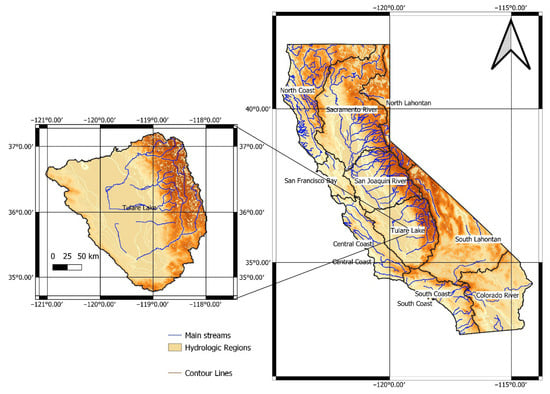
Figure 2. Map of the Tulare Lake Basin.

Conversely, Tulare Lake Bed, Upper Deer/Upper White, and Upper Poso are the watersheds that receive less precipitation. Upper Deer/Upper White receives 208 mm on average, while the Tulare Lake Bed receives 211 mm, and Upper Poso, 248 mm. This represents 43, 42, and 32% less precipitation than the average for the entire watershed, respectively. These watersheds are found in the low part of the hydrologic region.

Both hydrologic regions have similar mean annual precipitation (365 for Tulare and 385 for Nazas–Aguanaval), and both exhibit important differences across subbasins. Asymmetries in precipitation are higher in the Tulare Lake Basin than in the Nazas–Aguanaval. Another difference between these watersheds is the period of precipitation. Precipitation in Nazas–Aguanaval occurs between June and September, while the opposite happens in Tulare Lake, where precipitation occurs between December and March. Another important difference is that in Tulare, precipitation is accumulated in the Sierra Nevada as snowpack, while that does not happen at Nazas–Aguanaval. This means that time lags between precipitation and runoff are significantly longer at Tulare.

In the Tulare Lake HR, 69% of water used is groundwater [8], while according to REPDA, groundwater use in the Nazas–Aguanaval watershed is 51%. In both cases, the original ecological character of the area has been changed dramatically, largely from the taming of local rivers for farming [13]. In addition, both are endorheic basins, and their lakes have virtually disappeared.

Statewide, the Tulare Lake Hydrologic Region shows the highest fraction of wells with decreasing groundwater storage [13], with the Nazas–Aguanaval watershed also exhibiting a large number of wells with decreasing water storage. From 2005 through 2019, there was an average annual reduction of 1110 hm³ (900 TAF) to 2590 hm³ (2100) TAF in the Central Valley, with almost 50% of the reduction occurring in the Tulare Lake Hydrologic Region [13].

Groundwater overdrafting does not influence water availability only. Another shared challenge for both areas is subsidence. More than 5150 km² (2000 mi²) in the Tulare Lake HR experienced subsidence of 7.62 to 91.4 cm (0.25 to 3 ft), with a maximum rate of 45.7 cm/yr (1.5 ft/yr) (8). A correlative problem for overdrafting, present in both watersheds, is arsenic pollution, which has important implications for public health [14,15].

Finally, from the economic and food security point of view, both watersheds are critical for the dairy industry. Ninety percent of California’s milk supply is produced in San Joaquin Valley, and the four counties located in the Tulare HR provided 54% of the milk produced in California in 2017 [16], while 20% of the milk production in Mexico comes from the Nazas–Aguanaval watershed [17]. The Nazas–Aguanaval watershed is home to 1.6 million people in the Laguna metropolitan area. Water supply comes from the main aquifer of the region, although an ongoing infrastructure project is looking to substitute this demand with surface water. The Nazas–Aguanaval region has 11 urban water utilities. Comparatively, the Tulare Lake Basin is home to four million people in multiple counties, including Tulare, Kings, Kern, and Fresno. The TLB has an estimated 355 community drinking water systems, with 80% of them serving fewer than 500 people, and 23 urban water suppliers. In both watersheds, urban water suppliers serve the same average number of people.

In 2016, the total irrigation area in the Tulare Lake Hydrologic Region reached 1.25 million hectares. Almonds and pistachios accounted for the largest share (23%), followed by grain (16%), grapes (11%), corn (10%), citrus (8%), and alfalfa (7%). The remaining 25% is divided into 12 other crops. This pattern contrasts significantly with that of Nazas–Aguanaval. Rangelands produce 70% of the forage crops [18]. However, the TLB maintains significant dairy production despite lacking forage crops, showing a clear priority for high-value perennial crops.

Mexico centralizes water management and major infrastructure operations under Conagua. Conagua organizes its staff in national, regional (watershed), and local (state) offices. Watershed Councils collaborate with regional offices, incorporating water users. They participate in the definition of water policy objectives and development of watershed plans. Sometimes, Technical Committees of Groundwater (COTAS, in Spanish) aid Water Councils; these are created for specific aquifers. Interestingly, Mexico’s first water-user association was formed in the Nazas–Aguanaval watershed in August 1990, approving the Regulation Decree for the MARL [19].

On the other hand, water management in the United States is decentralized because responsibilities are distributed among federal, state, and local governments [20]. The Sustainable Groundwater Management Act (SGMA) was approved in 2014 with the underpinning principle that groundwater management is better coordinated at the local level [13]. This Act created the Groundwater Sustainability Agencies (GSAs) and Groundwater Sustainability Plans (GSPs). GSAs receive technical support from California’s Department of Water Resources (DWR) for developing their GSPs and are subject to strict surveillance and feedback from NGOs, users’ associations, other government agencies, companies, and the general public.

One important difference is the geographical extent of the groundwater organizations. The COTAS is established for every aquifer. For example, the main aquifer of the Nazas–Aguanaval watershed has a surface of 12,616 km², while the groundwater subbasin of Kings has a surface of 3962 km². Even so, there is only one COTAS in charge of the MARL, and the groundwater subbasin of Kings has seven GSAs (with 566 km² of jurisdiction each, on average). Another important aspect is that the COTAS has no authority to develop and implement plans and projects; it can only participate as a collegiate body in the formulation of studies of the aquifer but is not to interfere with the implementation of projects and groundwater management, which limits its impact.

Since the recognition of the Human Right to Water in the Mexican Constitution in 2012, there has been a legal vacuum awaiting a General Law of Water. This has increased the debate over institutional arrangements in Mexico and can represent an opportunity to reflect on the current objectives of the COTAS and the Watersheds Councils, strengthen their structure, and direct them to achieve the objective of managing water with a watershed approach.

Groundwater basins in California are subjected to the Sustainable Groundwater Management Act (SGMA) of 2014, which requires users to develop and implement plans for achieving different sustainability goals regarding groundwater. Sustainability goals are defined based on the absence of six undesirable results. For the Tule groundwater basin, the undesirable results out of these six are chronic lowering of groundwater levels, reduction in groundwater storage, degraded water quality, and land subsidence. In addition, Groundwater Sustainability Agencies (GSAs) are created with the aim of developing and implementing Groundwater Sustainability Plans (GSPs).

There are 29 GSAs in the Tulare Lake Hydrologic Region, and of these, only nine GSPs have been approved, seven of which belong to the Kings Subbasin: Central King, North Fork King, South King, McMullin Area, Kings River East, North Kings, and James. Conversely, in the Nazas–Aguanaval watershed, there are 26 aquifers within hydrologic region 36. Only five Technical Committees on Groundwater have been formed for the following aquifers: Main, Aguanaval, El Palmar, General Cepeda-Sauceda, and Sain Alto.

Projects proposed in the approved GSPs are divided into six categories: conjunctive use, surface water, land management, groundwater use restrictions, water conservation and management of water via supply and demand. In addition, they are classified according to the estimated time to potential implementation. Alternatives for a time horizon >5 years are developing new surface water storage and urban water recycling. The former is determined by the time required to develop the infrastructure, while the latter is based on the time required for social assimilation of water recycling. Different alternatives proposed for the Kings Subbasin are reported in Table 1. Essentially, the sustainability goal of this plan is to ensure that, by 2040, the basin is being managed to maintain a reliable water supply for current and future beneficial uses without experiencing undesirable results. This will be achieved by balancing water demand with available supply and by correcting and ending the long-term trend of a declining water table.

Table 1. Projects formulated for and/or implemented in the Kings Subbasin, California, classified by category and planning time horizon.

Category of Project	0–1 Years	1–5 Years
Conjunctive use	None	Groundwater recharge
		Groundwater banking
		Intentional irrigation field flooding
Surface water	Fully utilize surface water allocation	Direct use of flood and storm water
	Internal surface water trading	Import new surface water supplies
	Take or pay pricing structure	Develop conveyance capacity
	Low surface water pricing
Land management	Crop conversion	Agricultural land conversion
		Expand districts
	Deficit irrigation	Subsidies
		Disclaimer for property purchases
	Urban land use regulations	Prohibition of land development
Groundwater use restrictions	Prohibit groundwater exports
	Groundwater metering and pumping restrictions
	Additional well permit requirements
	Prohibition of composite wells
	Domestic well mitigation program
Water conservation	Water use restrictions in droughts	Industrial water recycling
	Agricultural water conservation
	Urban water conservation
	Water conservation credits	Agricultural water recycling
	Tiered pricing
	Groundwater pumping fees
	Wellhead fees
Others	Groundwater credits	Water desalination
		Blend poor and good quality water
	Public education	Use produced water
		Rainwater harvesting

Conversely, in the Nazas–Aguanaval watershed, an important infrastructure program is under construction. The program includes a small dam, a pumping station, a potabilization plant, aqueducts, storage tanks, and distribution pipelines. Essentially, the objective of this program is to substitute groundwater with surface water within the watershed and reduce hidroarsenicism and pressure in the aquifer. The Nazas–Aguanaval then faces a challenge of water sustainability. The main aquifer is overdrafted, and surface water is completely compromised for different uses. If more surface water is to be reallocated from agricultural to urban use, then there is a need to reduce the consumption of water from the irrigation district. This will eventually reduce pressure on the main aquifer. The Nazas–Aguanaval watershed shares the sustainability goal of maintaining a reliable water supply for both agriculture and urban water uses and reversing the long-term trend of a declining water table.

Some of the management actions that have been proposed in approved GSPs for the Kings Subbasin have already been proposed or implemented in La Laguna. A pilot study of Managed Aquifer Recharge (MAR) that proved the technical feasibility of the technique was previously conducted [21], but the plan has not been implemented at full scale because of insufficient social and financial support [22]. The adoption of deficit irrigation has been limited because of low technical assistance, scarce awareness of government programs, and current incomes and education levels [23]. Since the main aquifer of La Laguna does not have water available, concessions cannot be made. The Agua Saludable para La Laguna project includes the development of conveyance and storage capacity, utilization of surface water allocation, efficiency increases in houses, and a water treatment plant. When finished, this project will use 200 hm³/year that was previously assigned to the 017 irrigation district.

If water supply demand is to increase in the future because of population growth, a higher volume of water than is currently used by agriculture will be required. One of the alternatives that has been recently explored is crop reconversion and the establishment of a water pricing policy [17]. In La Laguna, a policy of this kind would decrease the demand for agriculture use, liberating water resources for urban supply purposes and releasing pressure on the main aquifer, preventing subsidence and arsenic pollution. In addition, given the hydrologic variability of La Laguna, drought scenarios can be expected. This supports the application of an optimization model for agriculture use.

Previously, it has been argued that forage crops should not be planted in this region [17]. Although a transition from these kinds of crops is possible in the long term, there is an urgency to modify the cropping patterns to reduce water use in the short term. For that reason, the proposal considers scenarios that preserve forage crop production.

2.2. Hydro-Economic Model

Agriculture data, including crop prices, production costs, and yields, were retrieved from the Agriculture Information System (Sistema de Información Agroalimentaria de Consulta) (SIACON) from the Agriculture Secretariat of Mexico and the Central Bank’s FIRA (instituted trust related to agriculture). All prices were updated to real terms using annual inflation rates. The analysis was conducted for ID 017 using the 2022 cropping pattern as the baseline scenario. The search was conducted using the 35 municipalities that are found within the watershed (6 in Coahuila, 21 in Durango, and 8 in Zacatecas). Data handling, processing and computation was done using Excel 2510.

2.3. Blaney–Criddle Computation

Based on previous identification of crops that are irrigated in the Nazas–Aguanaval watershed, evapotranspiration was computed using the Blaney–Criddle model following the procedure indicated in (1). Conduction and distribution efficiency was considered to be 0.55, as reported in [24]. The justification for using the Blaney–Criddle method over more complex methods, such as Penman–Monteith and/or FAO-56, is its suitability for regional analysis under data constraints [25].

Evapotranspiration for month i is computed using Equation (1). Here, K_c is the partial development coefficient of the crop, P is the percentage of sun hours, and T is the mean monthly temperature.

$$E_{ti}={Kc}_i\left({\displaystyle \frac{P_i·\left(T+17.8\right)}{21.8}}\right)\left(0.03114·T+0.2396\right)$$

(1)

Net irrigation depth is computed as the sum of monthly net irrigation depths. The ratio of the raw irrigation depth to the efficiency of conduction and distribution yields the raw irrigation depth (or irrigation requirements). This value was used to compute applied water per unit area for each crop.

Sources for development coefficients of crops were retrieved from [26] for alfalfa, cotton, peanuts, maize, nuts, and tomato. For oats, sorghum, and melon, the coefficients were obtained from [27]. Dry and green chili coefficients were obtained from [28] and [29], respectively.

Price, cost, and yield data were retrieved from the datasets reported by the Mexico Central Bank via the trusts instituted in relation to agriculture (FIRA, in Spanish). All but two of the prices were from 2021, and those that were not were updated using annual inflation reported by Mexico Central Bank. Crops with the highest prices and costs per ton are nuts, dry chili, and cotton, while the lowest correspond to oats, sorghum, and maize. Crops with the highest yield and cost per hectare are tomato, green chili, and melon. These data, along with raw irrigation depth computed previously, are reported in Table 2. The crops with more water requirements are alfalfa, beans, and maize, and those with less are melon and chili.

Table 2. Agriculture data used for the Nazas–Aguanaval crops.

Crop	Scientific Name	Price (USD/Ton)	Yield (Ton/ha)	Revenue (USD/ha)	Cost (USD/ha)	Irrigated Crop Area (ha)	Raw Irrigation Depth (cm)
Alfalfa	Medicago sativa L.	USD 212	83	USD 17,576	USD 16,689	5157	299
Cotton	Gossypium hirstium L.	USD 2056	5	USD 10,279	USD 5817	11,256	118
Peanut	Arachis hypogaea	USD 882	2	USD 1765	USD 719	200	128
Green chili	Capsicum annuum L.	USD 212	16	USD 3388	USD 2484	133	119
Forage maize	Zea mays L.	USD 39	45	USD 1774	USD 1408	13,985	197
Grain maize	Zea mays L.	USD 247	6	USD 1482	USD 1051	531	197
Melon	Cucumis melo	USD 206	30	USD 6176	USD 3943	888	108
Nuts	Juglans regia	USD 4412	1	USD 4412	USD 3578	7726	169
Broom sorghum	Sorghum vulgare	USD 562	4	USD 2249	USD 1454	159	127
Forage sorghum	Sorghum vulgare	USD 40	46	USD 1840	USD 1619	16,307	127
Tomato	Solanum lycopersicum	USD 824	60	USD 49,412	USD 30,296	50	174

The analysis was conducted for irrigation district 017, which exclusively uses surface water. The base scenario is the cropping pattern of 2022, as reported in (4). In this district, between 2003 and 2022, the average irrigated area was 50,664 ha, with a minimum of 12,378 and a maximum of 71,964 in 2002 and 2011, respectively. During this period, crop yields showed little change, except for tomato, which experienced a threefold increase in yield, leading to a corresponding rise in production without expanding the irrigated area. The values used for computation were the averages for the period 2003–2021.

The irrigated area of alfalfa, oats, and grain maize has been relatively steady. Forage maize showed an increase from 2013 onwards, while forage sorghum exhibited a decrease during 2009–2016 and an increase from 2016 onwards. Conversely, in relative terms, the area cultivated with alfalfa remained around 11%, forage maize increased from 14% to 27%, and forage sorghum exhibited an increasing trend after 2016, reaching 27% of the crop mix by 2021 and becoming the most important crop in the watershed. In 2008, sorghum replaced alfalfa as the main crop in the watershed and remained as such throughout the following years. The share of forage crops in the cropping pattern increased from 33% in 2003 to 64% in 2021. Forage crop production increased from 787 thousand tons in 2003 to 1.77 million tons in 2021.

2.4. Positive Mathematical Programming (PMP)

With the increasing diversity of water users and the extent to which water is becoming scarcer, its use is necessarily associated with opportunity costs. This opportunity cost reflects the value of goods and services lost because of the allocation of water elsewhere. In the agriculture sector, the decreasing water availability forces the establishment of water policies to maximize water productivity or water allocation to maximize production value per unit of water. Usually, the cost of providing water to farmers is lower than the opportunity cost of using the scarce resource in other sectors of production or of increasing the irrigation area [30].

A useful approach for estimating this opportunity cost is the marginal value, or shadow price, of water [26,27]. Marginal value of water represents the increase in total value if one additional unit of water becomes available; when it equals the marginal cost of delivering water, it reaches economic efficiency [31]. In three studies in Mexico, these marginal values were found to be higher than the actual water fees for water supply [9,28,29].

Positive Mathematical Programming (PMP) is a self-calibrated deductive method that has important advantages over inductive methods for estimating the economic value of water [32,33]. These advantages are (1) that the cost function calibrates the model to the observed values of production output and production factor use, (2) that the method adds flexibility to the profit function by relaxing the restrictive linear cost assumption, and (3) that it does not require large datasets [34]. PMP has been successfully applied in irrigated agriculture in Mexico [6,28,29].

The validity of PMP is rooted in its fidelity to economic reality. PMP is consistent with microeconomic theory since it uses the farms’ existing crop patterns to create self-calibrating models [35]. PMP avoids unrealistic outcomes, yielding smooth calibration results [36]. Methodologically, PMP is designed to ensure existing crop pattern reproduction without the use of constraints difficult to justify based on economic theory and derives a non-linear quadratic cost function that aggregates the economic rationale of the farmers [35], making crop policies more realistic and feasible. PMP is used to discover plans that minimize economic losses from water scarcity [37].

Also, the choice of PMP is justified when contrasting it with alternative methods. PMP is typically compared to Linear Programming (LP) and econometric and statistical models. Unlike LP, which often results in the abandonment of a large number of existing crops, PMP succeeds in preserving existing crops and, hence, does not impose major changes to ongoing crop patterns [35]. In addition, econometric and statistical models are limited to observed historical data, while PMP allows for adaptation to technology, crop mixes, and land use possibilities [38]. Also, PMP is suitable for unprecedented conditions and eases the estimation of the shadow price [38].

PMP consists of three steps. In the first step, the sum of the net benefit of the district is maximized in a linear program subject to limited resources and calibration constraints. The net benefit Z is computed by subtracting the cost c_i from the product of the crop price P_i and crop yield y_i (Equation (2)). The limited resource (land and water) constraints are expressed in Equation (3) using the parameter b_j. A calibration constraint is added to force the linear program to the baseline (observed) land and water use values. The decision variables are subject to non-negativity constraints (Equations (4) and (5), respectively).

In the second step, the total cost function TC_k is parameterized (Equation (6)) and calibrated to the observed values of production and use of inputs by using the shadow price of the calibration constraints (Equation (4)). Finally, in the third step, the sum of total net benefits Z is maximized with a non-linear objective function, subject to land and water availability. The objective function is expressed in Equation (6). The constraints of the model are shown in Equations (9)–(11).

Step 1: Linear Calibration Program (LCP). The LCP maximizes the net benefit, subject to land and water resource availability and a calibration constraint that pushes the model to select the observed baseline values for each crop. This step’s output is the shadow price associated with the calibration constraint for each crop and represents the marginal opportunity cost of increasing the area of crops beyond the observed baseline.

$$Max Z=\sum _i\left(P_i{y}_i-c_i\right)x_i$$

(2)

$$i=\mathrm{c}\mathrm{r}\mathrm{o}\mathrm{p}, \mathrm{P}=\mathrm{C}\mathrm{r}\mathrm{o}\mathrm{p} \mathrm{p}\mathrm{r}\mathrm{i}\mathrm{c}\mathrm{e}, \mathrm{c}=\mathrm{p}\mathrm{r}\mathrm{o}\mathrm{d}\mathrm{u}\mathrm{c}\mathrm{t}\mathrm{i}\mathrm{o}\mathrm{n} \mathrm{c}\mathrm{o}\mathrm{s}\mathrm{t}, \mathrm{x}=\mathrm{D}\mathrm{e}\mathrm{c}\mathrm{i}\mathrm{s}\mathrm{i}\mathrm{o}\mathrm{n} \mathrm{v}\mathrm{a}\mathrm{r}\left(\mathrm{h}\mathrm{a}\right)$$

$$\mathrm{S}\mathrm{u}\mathrm{b}\mathrm{j}\mathrm{e}\mathrm{c}\mathrm{t} \mathrm{t}\mathrm{o}:$$

$$\sum _i{a}_i{x}_i\le b_j \forall j$$

(3)

$$a=\mathrm{T}\mathrm{e}\mathrm{c}\mathrm{h}\mathrm{n}\mathrm{i}\mathrm{c}\mathrm{a}\mathrm{l} \mathrm{c}\mathrm{o}\mathrm{e}\mathrm{f}\mathrm{f}\mathrm{i}\mathrm{c}\mathrm{i}\mathrm{e}\mathrm{n}\mathrm{t}, b=\mathrm{l}\mathrm{i}\mathrm{m}\mathrm{i}\mathrm{t} \mathrm{i}\mathrm{n} \mathrm{p}\mathrm{r}\mathrm{o}\mathrm{d}\mathrm{u}\mathrm{c}\mathrm{t}\mathrm{i}\mathrm{o}\mathrm{n} \mathrm{i}\mathrm{n}\mathrm{p}\mathrm{u}\mathrm{t}, \mathrm{j}=\mathrm{l}\mathrm{i}\mathrm{m}\mathrm{i}\mathrm{t}\mathrm{e}\mathrm{d} \mathrm{r}\mathrm{e}\mathrm{s}\mathrm{o}\mathrm{u}\mathrm{r}\mathrm{c}\mathrm{e}\mathrm{s}, \mathrm{w}\mathrm{a}\mathrm{t}\mathrm{e}\mathrm{r} \mathrm{l}\mathrm{a}\mathrm{n}\mathrm{d}$$

$$\mathrm{C}\mathrm{a}\mathrm{l}\mathrm{i}\mathrm{b}\mathrm{r}\mathrm{a}\mathrm{t}\mathrm{i}\mathrm{o}\mathrm{n} \mathrm{c}\mathrm{o}\mathrm{n}\mathrm{s}\mathrm{t}\mathrm{r}\mathrm{a}\mathrm{i}\mathrm{n}\mathrm{t}:x_i\le \overline{x_i}+\epsilon$$

(4)

$$\overline{x_i}=\mathrm{O}\mathrm{b}\mathrm{s}\mathrm{e}\mathrm{r}\mathrm{v}\mathrm{e}\mathrm{d} \mathrm{v}\mathrm{a}\mathrm{l}\mathrm{u}\mathrm{e} \mathrm{o}\mathrm{f} \mathrm{p}\mathrm{r}\mathrm{o}\mathrm{d}\mathrm{u}\mathrm{c}\mathrm{e}\mathrm{d} \mathrm{h}\mathrm{e}\mathrm{c}\mathrm{t}\mathrm{a}\mathrm{r}\mathrm{e}\mathrm{s}$$

$$\mathrm{N}\mathrm{o}\mathrm{n}-\mathrm{n}\mathrm{e}\mathrm{g}\mathrm{a}\mathrm{t}\mathrm{i}\mathrm{v}\mathrm{i}\mathrm{t}\mathrm{y} \mathrm{c}\mathrm{o}\mathrm{n}\mathrm{d}\mathrm{i}\mathrm{t}\mathrm{i}\mathrm{o}\mathrm{n}:x_i\ge 0 \forall$$

(5)

Step II: Estimating quadratic cost function. The model assumes a quadratic total cost function for each crop and defines the marginal cost as the derivative of the total cost function. Lastly, the model assumes that farmers have an incentive to maximize profits, meaning that the marginal revenue must equal marginal cost.

$${TC}_k\left(x_{k,land}\right)={\alpha }_i{x}_{k,land}+{\displaystyle \frac{1}{2}}{\gamma }_i{x}_{k,land}^2$$

(6)

$${\alpha }_k=c_k-{\mu }_{k }$$

(7)

$$\alpha =\mathrm{I}\mathrm{n}\mathrm{t}\mathrm{e}\mathrm{r}\mathrm{c}\mathrm{e}\mathrm{p}\mathrm{t}, \gamma =\mathrm{C}\mathrm{a}\mathrm{l}\mathrm{i}\mathrm{b}\mathrm{r}\mathrm{a}\mathrm{t}\mathrm{i}\mathrm{o}\mathrm{n} \mathrm{p}\mathrm{a}\mathrm{r}\mathrm{a}\mathrm{m}\mathrm{e}\mathrm{t}\mathrm{e}\mathrm{r}\left(MR=MC\right), \mu =\mathrm{S}\mathrm{h}\mathrm{a}\mathrm{d}\mathrm{o}\mathrm{w} \mathrm{p}\mathrm{r}\mathrm{i}\mathrm{c}\mathrm{e}$$

Step III: Calibrated non-linear optimization program. This step assumes that the final solution will maximize profit under land and water constraints, using the cost function derived in Step II.

$$Max Z=\sum _k\left(P_k{y}_k\right)x_{k,land}-\sum _k\left({\alpha }_k+{\displaystyle \frac{1}{2}}{\gamma }_k{x}_{k,land}\right)x_{k,land}-\sum _k\left({\alpha }_k+{\displaystyle \frac{1}{2}}{\gamma }_k{x}_{k,land}\right)x_{k,land}$$

(8)

$$\mathrm{S}\mathrm{u}\mathrm{b}\mathrm{j}\mathrm{e}\mathrm{c}\mathrm{t} \mathrm{t}\mathrm{o}:$$

$$\sum _i{a}_{k,land}{x}_{k,land}\le b_{k,land} \forall k,land$$

(9)

$$\sum _i{a}_{k,water}{x}_{k,land}\le {\delta b}_{k,water} \forall k,water$$

(10)

$$x_{k,land}\ge 0 \forall i,land$$

(11)

Step IV: Calibrated non-linear optimization program for incorporating water price. This was an added step in the calibration process necessary for running the policy scenarios. The purpose of this step is to estimate the impact of different water pricing policies on the optimal cropping pattern. This is essentially Step III but with the water price added to the objective function. In this step, the water price is assumed to be fixed, and it is assumed that farmers will act rationally by adjusting cropping areas to maximize profits. Lastly, we assume that the price of water does not impact market prices of agricultural products.

$$Max Z=\sum _k\left(P_k{y}_k\right)x_{k,land}-\sum _k\left({\alpha }_k+{\displaystyle \frac{1}{2}}{\gamma }_k{x}_{k,land}\right)x_{k,land}-\sum _k{P_w{AW}_{k}x}_{k,land}$$

(12)

$$P_w=\mathrm{P}\mathrm{r}\mathrm{i}\mathrm{c}\mathrm{e} \mathrm{o}\mathrm{f} \mathrm{w}\mathrm{a}\mathrm{t}\mathrm{e}\mathrm{r} \mathrm{c}\mathrm{o}\mathrm{s}\mathrm{t}\left({\displaystyle \frac{\mathrm{U}\mathrm{S}\mathrm{D}}{\mathrm{d}\mathrm{a}\mathrm{m}3}}\right), {AW}_k=\mathrm{A}\mathrm{p}\mathrm{p}\mathrm{l}\mathrm{i}\mathrm{e}\mathrm{d} \mathrm{w}\mathrm{a}\mathrm{t}\mathrm{e}\mathrm{r} (\mathrm{c}\mathrm{m})$$

For every policy scenario, additional constraints were considered in addition to those in Step 3, including a fixed production of 1.8 million tons of forage crops, a minimal production of nuts and alfalfa (7000 and 5000 ha, respectively), an increase in water distribution efficiency (from 0.55 to 0.60, 0.65, and 0.70), and an increase in crop yield (5, 10, 15, and 20%). Water and land availability are defined by 2022’s water use, estimated at 927 hm³ and 56,392 ha, respectively. Scenario 1 consists of only having water and land restrictions. This is a laissez-faire scenario, since only water and land scarcity drive the behavior of farmers, without any policy. This informs the design of water pricing policies and establishes the economic baseline for the study. Scenario 2 reflects the economic needs to support the dairy value chain while simultaneously addressing water scarcity. In addition, this model will determine the minimum water availability for sustaining current forage production levels and measure the opportunity cost of allocating water resources to this activity. Scenario 3 is included to test the sustainability and economic cost of potential future growth of the dairy sector in the Nazas–Aguanaval watershed and the consequent need for more forage production.

To maintain farming profits under water scarcity, Scenario 4, maintaining nut production, is simulated. Nuts are a high-value crop in the Nazas–Aguanaval watershed, and hence, a rational policy could aim to preserve their cultivation to maintain overall farming profits. In addition, the decision to remove nut trees has a significant land opportunity cost, since removing these trees requires a year of reconditioning the land. Lastly, this scenario is grounded in current trends, which have shown that the irrigated area for nuts is increasing.

Scenario 5 builds on the rationale for Scenario 4 of preserving high-value crops. Recent research proposes substituting the current forage cropping pattern [17]. However, forage crops have economic importance, and in particular, alfalfa is preferred in semiarid and arid climates like that of the Nazas–Aguanaval watershed because of its high nutritive value, yield potential, soil benefits, adaptability, and economic value [39]. Additionally, shifting to other forage crops can be difficult because of deep-rooted habits for irrigating alfalfa. Hence, this is a pragmatic policy to maintain an important component of the local dairy value chain, as well as reduce disruptions to ongoing agriculture practices.

Scenario 6 is included to test the effect of infrastructure modernization policy by simulating its effects on distribution efficiency. Increasing efficiency of distribution in the water district main increases yield per unit of water applied while conserving water. Current efficiency is estimated at 0.55; thus, the model runs considering three levels of efficiency improvements, namely, 0.60, 0.65, and 0.70.

Scenario 7 is included to test the efficacy of non-structural policy measures, focused on the technological development and implementation.

Similarly, increasing crop yield due to cultural practices or improvements in crop varieties would likely increase profits while preserving water resources and irrigated area.

It is important to note that, from a hydrologic perspective, this model operates with a fixed input since it is not coupled with a rainfall–runoff model and, hence, treats water availability as predetermined. The simulation is applied to irrigation district 017 of Nazas–Aguanaval, which is supplied with surface water. Scenarios are summarized in Table 3.

Table 3. Labels and descriptions of PMP scenarios.

Scenario ID	Description
Baseline Scenario 1 (WL)	Full water (927 hm3) and land availability (56,392 ha)
Scenario 2 (WLF)	Scenario 1 + forage production of minimum 1.8 million tons
Scenario 3 (WLFF_200, WLFF_225, WLFF_250, WLFF_275, WLFF_300)	Scenario 1 + Increasing forage production minimum (2.0, 2.25, 2.50, 2.75, and 3.00 million tons)
Scenario 4 (WLFN)	Scenario 2 + Minimum nut production of 7000 ha
Scenario 5 (WLFNA)	Scenario 4 + Minimum alfalfa production of 5000 ha
Scenario 6 (WLFNAE_60, WLFNAE_65, WLFNAE_70)	Scenario 5 + Different values of efficiency of the water district (0.60, 0.65, and 0.70)
Scenario 7 (WLFNAY_5, WLFNAY_10, WLFNAY_15, WLFNAY_20)	Scenario 5 + Increases in crop yields (0.05, 0.10, 0.15, and 0.20)

The procedure was repeated but considering five different water pricing policies, following Equation (12). Five policies were simulated. In the first one, a water cost of 94 USD/ha was maintained. This represents roughly 6 USD/dam³, which is the current price that is independent of consumption or crop type. In the second one, a volumetric cost depending on the raw irrigation depth of every crop was considered, as indicated in Table 4. This simulates a step towards volumetric price, where the cost varies depending on the irrigation depth of each crop.

Table 4. Policy alternatives for water costs per hectare for every crop in ID017.

Policy Scenario	Baseline	P6	P14	P21
Water price (USD/dam3)	6	6	14	21
Alfalfa	USD 94	USD 171	USD 422	USD 616
Cotton	USD 94	USD 67	USD 166	USD 242
Peanut	USD 94	USD 73	USD 181	USD 264
Green chili	USD 94	USD 68	USD 168	USD 245
Forage maize	USD 94	USD 113	USD 279	USD 406
Grain maize	USD 94	USD 113	USD 279	USD 406
Melon	USD 94	USD 62	USD 152	USD 222
Nuts	USD 94	USD 96	USD 238	USD 347
Broom sorghum	USD 94	USD 73	USD 180	USD 262
Forage sorghum	USD 94	USD 73	USD 180	USD 262
Tomato	USD 94.12	USD 99.59	USD 245.76	USD 358.41

In the third, the minimum shadow price identified in the previous section was considered (14 USD/dam³). This represents a policy proposal with a floor price that reflects the resource’s minimum opportunity cost. In the fourth policy, shown in Table 5, the water tariff was based on the shadow price, which depends on water availability. As a result of the simulation of the fourth policy, a break-even or positive net returns price was estimated at 45 USD/dam³. Hence, this is a high-cost recovery policy. Policy 5 employs a price of 21 USD/dam³, which is the sum of the previous section’s weighted average price (6 USD/m³) plus the minimum shadow price (14 USD/dam³), which could be politically feasible, as it reflects both farmers’ willingness to pay and the current price. Lastly, a policy based on shadow prices and adjusted for positive profits is indicated in Table 6. In every scenario that considers a fixed cost, the shadow price is higher than the price currently charged (6 USD/dam³, or 94 USD/ha).

Table 5. Water costs per hectare for policy alternative 4, based on shadow prices (P4_SPF).

Water Availability	100%	95%	90%	85%	80%	75%	70%
Alfalfa	USD 171	USD 171	USD 419	USD 1350	USD 6496	USD 12,228	USD 18,601
Cotton	USD 67	USD 67	USD 165	USD 530	USD 2551	USD 4802	USD 7305
Peanut	USD 73	USD 73	USD 180	USD 579	USD 2787	USD 5245	USD 7978
Green chili	USD 68	USD 68	USD 167	USD 536	USD 2582	USD 4860	USD 7392
Forage maize	USD 113	USD 113	USD 277	USD 891	USD 4286	USD 8067	USD 12,271
Grain maize	USD 113	USD 113	USD 277	USD 891	USD 4286	USD 8067	USD 12,271
Melon	USD 62	USD 62	USD 151	USD 486	USD 2340	USD 4406	USD 6702
Nuts	USD 96	USD 96	USD 236	USD 760	USD 3660	USD 6888	USD 10,477
Broom sorghum	USD 73	USD 73	USD 179	USD 575	USD 2768	USD 5209	USD 7924
Forage sorghum	USD 73	USD 73	USD 179	USD 575	USD 2768	USD 5209	USD 7924
Tomato	USD 100	USD 100	USD 244	USD 785	USD 3779	USD 7113	USD 10,819

Table 6. Water costs per hectare for policy alternative 6 (P6_SPT), based on shadow prices and adjusted for positive profits.

Water Availability	100%	95%	90%	85%	80%	75%	70%
Alfalfa	USD 176	USD 176	USD 422	USD 1356	USD 1356	USD 1356	USD 1356
Cotton	USD 69	USD 69	USD 166	USD 532	USD 532	USD 532	USD 532
Peanut	USD 76	USD 76	USD 181	USD 581	USD 581	USD 581	USD 581
Green chili	USD 70	USD 70	USD 168	USD 539	USD 539	USD 539	USD 539
Forage maize	USD 116	USD 116	USD 279	USD 894	USD 894	USD 894	USD 894
Grain maize	USD 116	USD 116	USD 279	USD 894	USD 894	USD 894	USD 894
Melon	USD 63	USD 63	USD 152	USD 488	USD 488	USD 488	USD 488
Nuts	USD 99	USD 99	USD 238	USD 764	USD 764	USD 764	USD 764
Broom sorghum	USD 75	USD 75	USD 180	USD 577	USD 577	USD 577	USD 577
Forage sorghum	USD 75	USD 75	USD 180	USD 577	USD 577	USD 577	USD 577
Tomato	USD 102	USD 102	USD 246	USD 788	USD 788	USD 788	USD 788

3. Results

The results are reported as the fraction of water available in comparison with 2022’s availability. This fraction can represent a water policy that seeks to liberate water volume for other uses or a drought situation, where water availability is compromised. In any case, this approach reflects the physical scarcity of water.

3.1. Scenario 1: Only Water and Land Restrictions (WL)

Scenario 1 consists of only having water and land restrictions. The water availability is set at 927 hm³ and the land availability at 56,392 ha, representing the respective values observed in 2022. A set of models considers a range of water availability from 100 down to 5%. The shadow price does not change between 100 and 90% (16 USD/dam³), shifts to 19 USD/dam³ between 85 and 50% and increases at a higher rate below 45% availability, amounting to 420 USD/dam³ at 5% water availability.

The cropping pattern analysis shows that substituting forage maize with sorghum is necessary to maintain water resources and profits. In contrast, permanent crops such as nuts, which occupy 7726 ha, do not share a significant footprint in production and have higher per-unit net returns, keeping overall crop profits high compared to other crops.

Between 100 and 90% water availability, it is possible to preserve total cultivated area at 56,342 ha, reflecting 2022’s observed values. Forage sorghum contribution to the cropping pattern is increased to a peak of 29,554 ha at 90% availability, at the expense of forage maize, which drops to zero by the 85% availability level.

Melon and cotton contributions to the cropping pattern are preserved at 8888 ha and 11,256 ha, respectively, for all values of water availabilities down to 45%, given their higher net returns. From a relative perspective, the priority crop in this ID is alfalfa, whose production is preserved at 5157 ha down to 90% availability. However, below 45% water availability, such a level of production is not sustainable and starts decreasing linearly from 4443 ha to zero below 30% availability. This is illustrated in Figure S1. Total forage production decreases from 1,809,399 tons at 100% availability to 5,177,777 tons at 50% availability, ceasing entirely below 30% availability.

3.2. Scenario 2: 2021 Observed Forage Production (WLF)

This scenario was designed to evaluate the constraints of preserving 2022’s observed forage production, which was set at 1.8 million tons. This reflects the economic necessity of supplying forage crops in this watershed; despite their relative lower value per unit area, these crops are fundamental elements and belong to an important value chain in the dairy industry.

Model results indicate that the minimum water availability for producing this amount of forage is 55%. This is the threshold at which the model can no longer maintain the required forage volume. This means that forage production at current levels is sustainable if the system does not face a water availability reduction exceeding 45%.

The shadow price starts at 16 USD/dam³ at 100% water availability, remains at this initial value down to 90% availability, and then reaches 542 USD/dam³ at 55%, as illustrated in Figure 3. The maximum recorded profit under this scenario is USD 76 million at 100% availability, decreasing to USD 21 million at 55% availability.

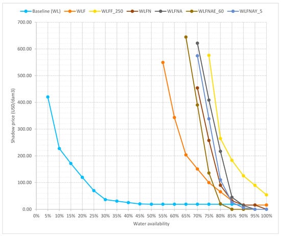
Figure 3. Shadow prices for different policy scenarios in ID017.

As in Scenario 1, sorghum production must be increased at the expense of maize for preserving forage production, as confirmed by the forage maize area dropping to zero at 85% availability and as shown in Figure S2. Below 90% availability, forage production keeps increasing its cultivated area at the expense of alfalfa, until reaching full forage production of sorghum at 75% water availability or less. The cultivated area of alfalfa decreases from 5157 ha at 100% availability to zero at 75% availability. Sorghum is a necessary substitute for forage production in this watershed if current levels of forage crop production are to be preserved. Forage sorghum’s cultivated area increases from 16,307 ha at 100% availability to a maximum of 38,723 ha at 75% availability.

3.3. Scenario 3: Increasing Forage Production (WLFF_200, WLFF_225, WLFF_250, WLFF_275, WLFF_300)

Between 1998 and 2011, average annual forage production was 1.34 million tons, with a maximum in 2009 (2.1 million tons) and a minimum in 2002 (282 thousand tons). After the 2011 drought, production decreased significantly, reaching a minimum in 2013, after which the trend increased. If forage production is to be increased, assuming there is no change in land or water availability or agricultural parameters, there will be limits to production. Given the increase in economic activity of the dairy industry, five sub-scenarios, where the production of forage crops increases from 2 (WLFF_200) to 3 million tons per year (WLFF_300), were modeled in 250,000 thousand tons increments.

A chart with the shadow prices is shown in Figure 4. Noticeably, to produce 2.0 million tons, 60% water availability is required, and full water availability is required to produce 3 million tons under this scenario. When production is increased, the shadow prices will increase as well. For WLFF_200, the shadow price increased from 14.04 USD/dam³ at 100% availability to 587.44 USD/dam³ at 60% availability. For WLFF_300, the shadow price reached 259.98 USD/dam³, even at 100% water availability.

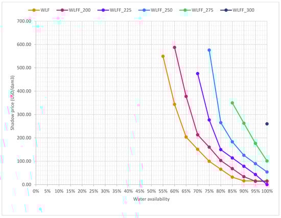
Figure 4. Shadow prices for different scenarios that involve an increase in forage crop production.

Profits decrease with increasing production of forage crops, suggesting that at least a fraction of other crops should be higher-value crops to maintain profitability. Total profit declined from USD 75 million for WLFF_200 to USD 51 million for WLFF_275, both for 100% water availability. For WLFF_300, profits dropped to USD 26 million at 100% water availability. This demonstrates the cost incurred when boosting forage production.

For production between 2.25 and 3.00 million tons, since the constraints of the model are severe, there is an incentive to just irrigate alfalfa to a small extent and maximize sorghum. If forage crop production is to be increased, the optimal policy is to prioritize forage sorghum over forage maize and alfalfa. In WLFF_200, forage sorghum area increased to a maximum of 43,025 ha at 75% availability, while alfalfa declined to zero at 75% and forage maize declined to zero at 90% availability.

In this scenario, 2.5 million tons of forage crops are produced, representing an increase of 28% in forage crop production with respect to 2022. This goal required a minimum of 70% water availability to be feasible, and the total cultivated area was 51,533 ha, and the profit was USD 52.4 million. The crop pattern is illustrated in Figure S3.

3.4. Scenario 4: Fixing Nut Production (WLFN)

Nuts’ irrigated area reached a maximum in 2021, when 7.8 thousand hectares was irrigated. For this scenario, the nut tree area was set to 7000 ha. Under this scenario, 70% water availability is necessary for feasibility. The shadow price increased from 0.00 at 100% availability to 453.95 USD/dam³ at 70% availability.

Unless water availability falls below 85%, the cropping pattern under this scenario does not compromise alfalfa or cotton production, as shown in Figure S4. Alfalfa production dropped from 7393 ha at 100% water availability and then declined to 9952 ha at 80%, and 3247 ha at 70% water availability.

3.5. Scenario 5: Fixing Nut and Alfalfa Production (WLFNA)

An alfalfa production area of at least 5000 hectares was set under this scenario, along with a fixed nut production area of 7000 ha. This scenario required a minimum of 70% water availability to be feasible. The scenario feasibility limit is defined by the 70% availability level. Preserving the level of production for nuts and alfalfa allows a 30% decrease in water availability from the baseline. This is illustrated in Figure S5.

The shadow price demonstrated a response to scarcity. The price remained 0.00 at 100% and 95% availability, and then increased to 14.15 USD/dam³ at 90% availability. It quickly escalated to 44.92 USD/dam³ at 85% availability, rising further to 621.51 at 70% availability.

The constraints imposed kept the alfalfa and nut areas within the intermediate range of water availability. Alfalfa was maintained at 5000 ha from 85% down to 70% availability. Analogously, nuts were kept at 7000 ha for the same interval. Total forage production was maintained at 34,824 ha from 85% down to 70% availability. Cultivation of more profitable, low-water-use crops ceased completely by 75% availability, including peanut (200 ha at 90% availability) and melon (887 ha at 90% availability). Cotton production declined consistently from 11,254 ha at 90% to 160 ha at 70% availability.

3.6. Scenario 6: Increasing Efficiency of the Water District (WLFNAE_60, WLFNAE_65, WLFNAE_70)

Three values for efficiency were included in this scenario: 0.60, 0.65, and 0.70. For the same water availability, the shadow price is higher when the efficiency is lower. At 75% water availability, for example, the shadow price ranged from 0.00 (WLFNAE_70) to 135.91 USD/dam³ (WLFNAE_60).

Maximum profits of USD 72 million can be preserved for water availability at 80% for the 0.60 scenario, 75% for the 0.65 scenario, and 70% for 0.70. However, profits are topped if no changes in technology or irrigation practices take place, as shall be discussed later.

Implementing this scenario would involve focusing on five specific crops: alfalfa, cotton, nuts, sorghum, and tomato, as shown in Figure S6. For all three efficiency values, cultivated areas of peanut, green chili, forage maize, grain maize, melon, and broom sorghum remain zero across all availability percentages. The irrigated area for red tomato is kept at 50 ha down to 75% availability for all three scenarios.

3.7. Scenario 7: Increasing Crop Yield (WLFNAY_5, WLFNAY_10, WLFNAY_15, WLFNAY_20)

Scenario 7 involved increases in crop yields under the fixed production constraints set in Scenario 5 (WLFNA), as shown in Figure S7. As in Scenario 6, implementing this policy would mainly involve prioritizing five crops: alfalfa, cotton, nuts, sorghum, and tomato. Marginal increases in yields were computed at four levels: 0.05, 0.10, 0.15, and 0.20.

An increase of 20% in yields of all crops involves an increase from the WLFNA baseline value of USD 74 million to USD 133 million at 100% water availability. This represents a range of USD 58.5 million between the baseline and the highest-yield scenario at 100% availability.

The shadow price did not change significantly at high water availability across the four yield values, remaining at 0 down to 90% availability. However, the scarcity threshold shifted. For the 0.05 yield increase, the shadow price reached 5.15 USD/dam³ at 90% availability, while for the 0.20 yield increase, the shadow price was kept at 0.00 at 90% availability but increased to 48.23 USD/dam³ at 85% availability, as shown in Figure 5. Total forage production was maintained at 413.645 tons of alfalfa and a varying amount of forage sorghum, fulfilling the base forage constraint.

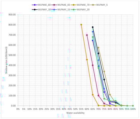
Figure 5. Shadow prices for policy scenarios that involve an increase in ID efficiency and crop yield.

4. Discussion

Forage crops are often characterized as low value with high water use intensity [17]. However, in this context, forage crops are an important subsector of agriculture in the Nazas–Aguanaval watershed and respond to ongoing market demand. Reconversion to other kinds of crops is feasible in principle, as has been implemented in the past when the watershed turned from cotton to forage crops, but this will only be possible in the long term, and the current water crisis in the Nazas–Aguanaval watershed must be addressed immediately. However, the evidence of effectiveness of crop reconversion for reducing water use is mixed, since there are reports that this has decreased water use in agriculture. For example, in the California Central Valley, where the TLB is located, up to 93% of reduction in water use was achieved [40]. Similarly, results from the Banas River Basin in India indicate that changing the cropping pattern would reduce water consumption [41].

Seven scenarios were compared. Within those, WLFF_250 was examined, as well as WLFNAE_60, representing a 0.6 improved distribution efficiency, and WLFNAY_5, which assumes an increase of 5% in crop yield. An increase in required forage production (WLFF_250) produces the highest shadow prices, followed by a policy of fixing alfalfa and nuts (WLFNA), given the high opportunity cost of other water uses under these restrictive scenarios. This is consistent with findings in the literature that report that this is due to forages being less profitable per unit of water used, and their large-scale production can lead to inefficient water allocation in watersheds [17,42,43].

The baseline scenario WF and WLF exhibit the lowest water shadow prices. A comparison of the cropping patterns for 100% water availability in all scenarios is shown in Figure 6.

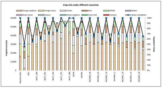
Figure 6. Crop mix under different policy scenarios for 100% water availability in ID 017.

The highest water shadow price is shown in Scenario WLFNAE_60, at 645 USD/dam³ at 65% availability, and the lowest non-zero water shadow price occurs for Scenario WL at 16 USD/dam³ at 100% availability. At 80% availability, the shadow price ranged between 19 and 265 USD/dam³. Previously, a value of 72 USD/dam³ was found [17].

Profit plots for the different scenarios are shown in Figure 7. Except for Scenarios WLFF_250 and WLFNAY_5, all the scenarios preserve the overall profits in the irrigation district across high water availability values. In Scenario WLFNAY_5, profits increase to a maximum of USD 87 million because of the increase in crop yield. This positive outcome validates and encourages investment in technology for improving productivity in the district. This is supported by the current literature, either through high-yielding varieties and improved seeds [44,45], genetically modified crops [46,47], mechanization [48], and/or sustainable practices [49,50,51]. Conversely, in Scenario WLFF_250, profits decline given an enforced increase in forage crop production. This decline occurs because land is limited, and more surface has to be devoted to this lower-value crop at the expense of higher-value crops. An optimal cropping pattern for the WL baseline scenario can reduce the relative profit loss with decreasing water availability, in comparison with the other scenarios. However, full water availability for sustaining current cropping patterns is not sustainable anymore because of water stress in this watershed.

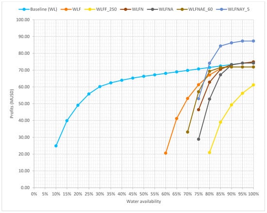
Figure 7. Profits for different water availability conditions and policy restrictions.

Considering the impact on profitability and the implementation suitability, we conclude that the most promising policy option for the Nazas–Aguanaval watershed in the short term is Scenario WLFNA. This scenario is appealing since it requires minimal infrastructure investment and reliance on short-term crop variety improvements. Scenario WLFNA requires a change in the cropping pattern and a cap on forage crop production. Cultivation in the irrigation district requires increases of between 44 and 74% in the land area devoted to alfalfa and forage sorghum, respectively, and eliminating forage maize and generating an 87% decrease in the area for grain maize. This approach to prioritizing high-value, fixed crops aligns with economic theory for water-scarce regions.

Price elasticities of demand for water are reported in Table 7 and range between −0.05 and −0.37, which are found in the lower range of those reported in [33]. Additionally, the mostly negative range is consistent with the literature [7,52,53], which reports that water price elasticity is typically found at negative levels but that it depends on the crop, region, and time frame. This narrow range of elasticity suggests that water demand in the Nazas–Aguanaval watershed is less sensitive to a change in price in comparison with other watersheds, such as irrigation district 11, in Guanajuato, Mexico. These elasticities may also reflect the small share of high-value crops and the artifact of constraining irrigated areas in some scenarios.

Table 7. Elasticity price of demand of water in ID017.

Elasticity	100%	95%	90%	85%	80%	75%	70%	65%
Scenario 1				−0.37
WLF				−0.12	−0.12	−0.19	−0.21	−0.30
WLFF_250		−0.13	−0.19	−0.19	−0.20	−0.12
WLFN		−0.05		−0.12	−0.10	−0.10	−0.17
WLFNA			−0.06	−0.09	−0.08	−0.14	−0.21
WLFNAE_60					−0.06	−0.08	−0.11	−0.19
WLFNAY_5			−0.06	−0.07	−0.08	−0.10	−0.17
Average		−0.09	−0.10	−0.16	−0.11	−0.12	−0.17	−0.25

The irrigation fee of ID017 is USD 94 ha⁻¹ [17,54]. This means that the fee is independent of the type of crop and the volume of water consumed. If a price per cubic meter is to be computed, the price must be divided by the actual applied water volume, which will vary from crop to crop. The irrigation fee (or price) did not change over the period covered in the published sources. This means that irrigation fee revenues have decreased in the last 20 years in real terms. The water prices are reported in Table 4. The market price of water will be lower for more water-intensive crops like alfalfa, maize, and tomato and higher for less water-intensive crops like melon and sorghum, given that the rate is by unit area (ha). The interval of weighted average prices for water is 7–11 USD/dam³. The fixed price of USD 94 ha⁻¹ was used to compute an average volumetric price for every crop, which constitutes the baseline scenario in Table 4.

Figure 8 shows the calculated change in profits by policy. The policies that maximize profits are P6 (tiered volumetric rate with 20% cap) and P14 (fixed rate of 14/dam³). The most abrupt reduction occurs with the tiered rate (P6_SPT). P4_SPF is reported partially because the model showed higher costs based on the shadow price, causing negative profits (or losses).

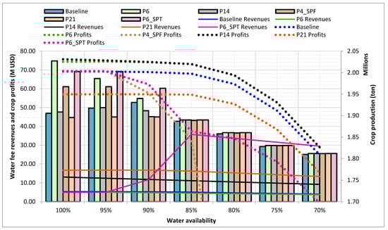
Figure 8. Profits, water fee revenues, and crop production for different pricing policies.

Figure 8 also shows changes in production. Policy P6 maximizes crop production, followed by P6_SPT and P4_SPF. All of them represent an increment with respect to baseline. Conversely, P14 and P21 reduce crop production with respect to baseline. As mentioned earlier, 1.8 million tons of forage crop production was fixed during the optimization. In addition, crop production is preserved between 1.80 and 2.05 million tons, which represents the highest relative production increase (14%).

The water rate of 94 USD/dam³ only covers a fraction of the irrigation district costs [17]. An increase in the water rate would likely raise additional revenue for the district that could be reinvested in infrastructure modernization. From a social perspective, the use of water pricing, together with the investment of revenue, is more beneficial for the whole [55]. The physical efficiency can increase, decreasing irrigation requirements for crops. Investments could also be made in infrastructure and practices that increase overall crop yields. In that sense, all policies represent higher revenues associated with water, compared to baseline.

P6 brings in less revenue because it considers a volumetric cost differentiated by crop. Analyzing revenue generation alone, P6_SPT is the policy that yields the highest revenue, reaching a maximum of USD 35 million at 85% water availability. At the same time, Policy P6_SPT results in the highest revenue losses for farmers. Policy P21 follows, and profit losses are highly correlated with water availability. P14 has higher revenue than baseline and also maximizes profits, yet a trade-off in production is needed. The implementation of this policy could represent increases ranging from 120 to 134 percent in gross agricultural revenue for the ID. Policy P14 is a fixed rate of 14 USD/dam³ and is considered the best policy for the irrigation district of the Nazas–Aguanaval watershed. In comparison, water fees in China range from 3 to 70 USD/dam³ [7,56,57], while in Australia, fees directed to water recovery were found in the range of 40 to 360 USD [58]

The first bar of Figure 9 shows 2022 cropping patterns, which is the business-as-usual (BAU) policy. The bars to the right are the modeled cropping patterns for the different values of water availability for the two water policies that were analyzed in this manuscript (WLFNA and P14). An initial observation indicates that the cropping patterns in the pricing policy and in the BAU policy are roughly the same. This suggests that the inclusion of a water price would not modify the incentives for profits in the BAU policy. However, when water availability decreases, there is an incentive to increase the share of forage sorghum in the mix at the expense of forage maize. This modeled behavior occurs despite the lower profit margin of 14% versus 26% for maize. If water availability keeps decreasing, the incentive is to reduce the planted area of cotton, decreasing the overall irrigated area in the ID.

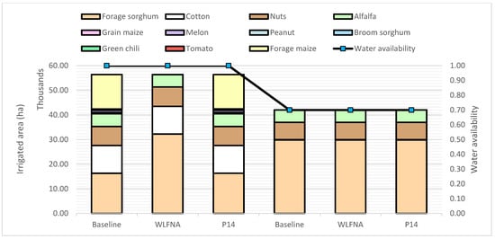
Figure 9. Comparison of baseline with proposed policies of cropping pattern shift and pricing for the highest and lowest water availability.

Limitations and Further Work

Some limitations of this research are worth discussing. First, the analysis was conducted at the irrigation district 017 level, the largest surface water user in the watershed. However, there are additional irrigation units outside of this irrigation district that presumably use groundwater to irrigate their crops. Conducting similar simulations for these units would deliver comparable policies on crop reconversion and water pricing for smallholders. Also, these entities could potentially participate in a cooperative scheme with the irrigation district, take advantage of economies of scale, and spread the costs of modernizing infrastructure.

On the other hand, financial data (market prices and production costs, for instance) from the crops was treated as a fixed variable. It is important to note that this data can vary over time. When considering important investments that are not subject to subsidies, such as the modernization of the irrigation district or development of higher-yielding seeds, the profit margin would decrease, and the optimal cropping pattern would be different. Similarly, there could be differences across yields, market prices, and the effects of the policy implementation. Considering this in further research would enhance the usefulness of the insights from this research.

The current optimization was performed for the entire Nazas–Aguanaval watershed, treating it as a single unit. Further research can focus on other water-stressed areas in Mexico and should also consider physical and water imports and exports between watersheds to formulate proposals for a water-rational agricultural policy that also maintains profits for farmers. The potential for developing water markets within modules in the irrigation district could be explored following the analysis in [33] to explore gains from trade as more granular information for Nazas–Aguanaval on cropping patterns and water deliveries becomes available.

Another limitation of the study is the fixed consideration of temperature and precipitation in the Blaney–Criddle computation of irrigation depth. While these factors are variable on an interannual basis, only an average was considered here. Failure to capture this variability means that the impact of higher temperatures and lower precipitation on crop irrigation needs could be underestimated.

Lastly, scenarios in which the irrigation district internalizes the increase in production costs associated with technological improvement and/or change in cultural practices are worthwhile exploring. Moreover, incorporating changes in crop prices might shift production incentives across farmers in the irrigation district and should also be analyzed in further work. Although increases in yield and water use efficiency have been considered, it is relevant to include the cost that both interventions represent in further research.

5. Conclusions

This study evaluated policies for increasing climate resilience in the water- and financially stressed Nazas–Aguanaval watershed of Mexico, using management experiences in the Tulare Lake Basin as a comparative framework.

The application of Positive Mathematical Programming (PMP) revealed that coordinated water and agriculture policy is essential for reconciling water scarcity with agriculture production and, hence, reconciling food security with water security. Specifically, the model demonstrated that water use reduction goals can be met most efficiently through a change in agriculture production priorities, rather than relying solely on volumetric reduction or the straightforward incorporation of technology. The analysis identified a clear strategy: first, implementing a crop pattern focused on high-value crops. This can reduce water demand by 20%, while capping profit losses at 11% relative to baseline.

The second part of the strategy is establishing a water price (14 USD/dam³) that could significantly increase the revenue of the irrigation district. These additional funds could be used for modernization of the irrigation district, thereby increasing efficiency and reducing irrigation requirements. The implementation of such a policy may foster continuous improvement.

These results underscore the value of cross-watershed analysis between comparable systems, such as the Nazas–Aguanaval and the Tulare Lake Basin, both of which face similar challenges related to groundwater overdrafting, subsidence, and increasing climate vulnerability. By providing policy proposals and demonstrating the economic viability of changing crop patterns and implementing water prices, this research delivers a model for implementation in watersheds that are under severe water and financial stress. Ultimately, these findings are crucial for increasing climate resilience and achieving water security worldwide.

References

- Mojid, M.A.; Mainuddin, M. Water-saving agricultural technologies: Regional hydrology outcomes and knowledge gaps in the Eastern Gangetic Plains—A review. Water 2021, 13, 636. [Google Scholar] [CrossRef]
- Viana, F.J.; Cunha, F.F.D.; Rocha, M.O.; Oliveira, J.T. Water rationalization in Brazilian irrigated agriculture. Agron. Sci. Biotechnol. 2022, 8, 1–15. [Google Scholar] [CrossRef]
- Tsagkoudis, D.; Zafeiriou, E.; Spinthiropoulos, K. Spatial and economic-based clustering of Greek irrigation water organizations: A data-driven framework for sustainable water pricing and policy reform. Water 2025, 17, 2242. [Google Scholar] [CrossRef]
- Mu, L.; Wang, Y.; Xue, B. The impacts of agricultural water pricing on sustainable agricultural production. Water Resour. Manag. 2024. [Google Scholar] [CrossRef]
- Medellín-Azuara, J.; Harou, J.J.; Howitt, R.E. Estimating economic value of agricultural water under changing conditions and the effects of spatial aggregation. Sci. Total Environ. 2010, 408, 5639–5648. [Google Scholar] [CrossRef] [PubMed]
- Chand, P.; Singh, J.M.; Sachdeva, J.; Singh, J.; Agarwal, P.; Jain, R.; Rao, S.; Kaur, B. Irrigation water policies for sustainable groundwater management in irrigated northwestern plains of India. Curr. Sci. 2022, 123, 1225. [Google Scholar] [CrossRef]
- Zhou, Q.; Zhang, Y.; Wu, F. Can water price improve water productivity? A water-economic-model-based study in Heihe River Basin, China. Sustainability 2022, 14, 6224. [Google Scholar] [CrossRef]
- Yao, J.; Berbel, J.; Yang, Z.; Wang, H.; Martínez-Dalmau, J. Application of positive mathematical programming (PMP) in sustainable water resource management: A case study of Hetao Irrigation District, China. Water 2025, 17, 2598. [Google Scholar] [CrossRef]
- Li, G.; Ma, D. Can a tiered water price policy improve the technical efficiency of crop irrigation for maize in the Heihe River Basin in Northwest China? Agric. Water Manag. 2025, 309, 109350. [Google Scholar] [CrossRef]
- Nikbakhsh, F.; Sabuhi Sabuni, M. Effects of trade liberalization policies on water resource management through the concept of water shadow price: Application of the DCGE model. Water Supply 2025, 25, 1001–1015. [Google Scholar] [CrossRef]
- Yang, X.; Hou, M.; Zhang, W.; Ju, Y.; Wang, Z. Optimization of agricultural water price setting strategy and government subsidy mechanisms based on game analysis. Agric. Water Manag. 2025, 319, 109814. [Google Scholar] [CrossRef]
- Dorjderem, B.; Torres-Martínez, J.A.; Mahlknecht, J. Intensive long-term pumping in the Principal-Lagunera Region aquifer (Mexico) causing heavy impact on groundwater quality. Energy Rep. 2020, 6, 862–867. [Google Scholar] [CrossRef]
- DWR. California’s Groundwater Update 2020. 2021. Available online: https://cawaterlibrary.net/wp-content/uploads/2021/05/calgw2020_chapters1_6.pdf (accessed on 28 October 2025).
- Mahlknecht, J.; Aguilar-Barajas, I.A.; Farias, P.; Knappett, P.S.K.; Torres-Martínez, J.A.; Hoogesteger, J.; Lara, R.H.; Ramírez-Mendoza, R.A.; Mora, A. Hydrochemical controls on arsenic contamination and its health risks in the Comarca Lagunera region (Mexico): Implications of the scientific evidence for public health policy. Sci. Total Environ. 2023, 857, 159347. [Google Scholar] [CrossRef]
- Smith, R.; Knight, R.; Fendorf, S. Overpumping leads to California groundwater arsenic threat. Nat. Commun. 2018, 9, 2089. [Google Scholar] [CrossRef] [PubMed]
- Matthews, W.A.; Sumner, D.A. Contributions of the California Dairy Industry to the California Economy in 2018. 2019. Available online: https://cail.ucdavis.edu/wp-content/uploads/2019/07/CMAB-Economic-Impact-Report_final.pdf (accessed on 28 October 2025).
- Ramírez-Barraza, B.A.; González-Estrada, A.; Valdivia-Alcalá, R.; Salas-González, J.M.; García-Salazar, J.A. Efficient rates for water for agricultural use in the Comarca Lagunera. Rev. Mex. Cienc. Agríc. 2019, 10, 3. [Google Scholar]
- Liu, H.; Jin, Y.; Roche, L.M.; O’Geen, A.T.; Dahlgren, R.A. Understanding spatial variability of forage production in California grasslands: Delineating climate, topography and soil controls. Environ. Res. Lett. 2021, 16, 014043. [Google Scholar] [CrossRef]
- Gutiérrez-Ojeda, C.; Escolero-Fuentes, O.A. Groundwater resources of Mexico. In Water Resources of Mexico; Springer: Cham, Switzerland, 2020. [Google Scholar]
- He, C.; Harden, C.P.; Liu, Y. Comparison of water resources management between China and the United States. Geogr. Sustain. 2020, 1, 98–108. [Google Scholar] [CrossRef]
- Gutiérrez-Ojeda, C.; Ortíz-Flores, G. Proyectos de recarga MAR en el acuífero principal de la región lagunera. In Manejo de la Recarga de Acuíferos: Un Enfoque Hacia Latinoamérica; IMTA-UNAM: Jiutepec, Mexico, 2017; pp. 139–157. [Google Scholar]
- Cruz-Ayala, M.B.; Megdal, S.B. An overview of managed aquifer recharge in Mexico and its legal framework. Water 2020, 12, 474. [Google Scholar] [CrossRef]
- Torres-Moreno, M.; Mora-Flores, J.S.; García-Salazar, J.A.; Rubiños-Panta, E.; Arana-Coronado, O.A.; Arjona-Suarez, E. Factores determinantes de la adopción de riego tecnificado en La Laguna, México. Tecnol. Cienc. Agua 2023, 14, 122–157. [Google Scholar] [CrossRef]
- Pedroza Gonzalez, E. Manejo y Distribución del Agua en Distritos de Riego: Breve Introducción Didáctica; IMTA: Jiutepec, Mexico, 2014. [Google Scholar]
- Abdelraouf, R.E.; El-Shawadfy, M.A.; Bakry, A.B.; Abdelaal, H.K.; El-Shirbeny, M.A.; Ragab, R.; Belopukhov, S.L. Estimating ETO and scheduling crop irrigation using Blaney–Criddle equation when only air-temperature data are available and solving the issue of missing meteorological data in Egypt. BIO Web Conf. 2024, 82, 02020. [Google Scholar] [CrossRef]
- Aparicio-Mijares, F.J. Fundamentos de Hidrología de Superficie; Limusa: Mexico City, Mexico, 1989. [Google Scholar]
- FAO. Evapotranspiración del Cultivo: Guías Para la Determinación de los Requerimientos de Agua de los Cultivos; FAO: Rome, Italy, 2006. [Google Scholar]
- Bravo Lozano, Á.G.; Galindo Gonzalez, G.; Amador Ramírez, M.D. Tecnología de Producción de Chile Seco; INIFAP: Mexico City, Mexico, 2006. [Google Scholar]
- Mata Vazquez, H. Cálculo de Volúmenes de Agua de Riego en el Cultivo de Chile. Método del Evaporímetro; INIFAP: Mexico City, Mexico, 2005. [Google Scholar]
- Palacios-Velez, E. Strategies to Improve Water Management in Mexican Irrigation Districts. Ph.D. Thesis, University of Arizona, Tucson, AZ, USA, 1976. [Google Scholar]
- Florencio-Cruz, V.; Valdivia-Alcalá, R.; Scott, C.A. Water productivity in the Alto Río Lerma (011) irrigation district. Agrocencia 2002, 36, 483–493. [Google Scholar]
- Medellín-Azuara, J.; Howitt, R.E.; Waller-Barrera, C.; Mendoza-Espinosa, L.G.; Lund, J.R.; Taylor, J.E. A calibrated agricultural water demand model for three regions in northern Baja California. Agrociencia 2009, 43, 83–96. [Google Scholar]
- Rodríguez-Flores, J.M.; Medellín-Azuara, J.; Valdivia-Alcalá, R.; Arana-Coronado, O.A.; García-Sánchez, R.C. Insights from a calibrated optimization model for irrigated agriculture under drought in an irrigation district on the Central Mexican High Plains. Water 2019, 11, 858. [Google Scholar] [CrossRef]
- Howitt, R.E.; Medellín-Azuara, J.; MacEwan, D.; Lund, J.R. Calibrating disaggregate economic models of agricultural production and water management. Environ. Model. 2012, 38, 244–258. [Google Scholar] [CrossRef]
- Moulogianni, C. Comparison of selected mathematical programming models used for sustainable land and farm management. Land 2022, 11, 1293. [Google Scholar] [CrossRef]
- Sapino, F.; Pérez-Blanco, C.D.; Gutiérrez-Martín, C.; Frontuto, V. An ensemble experiment of mathematical programming models to assess socio-economic effects of agricultural water pricing reform in the Piedmont Region, Italy. J. Environ. Manag. 2020, 267, 110645. [Google Scholar] [CrossRef]
- Trail, S.M.; Ward, F.A. Uniting agricultural water management, economics, and policy for climate adaptation through a new assessment of water markets for arid regions. Agric. Water Manag. 2024, 305, 109101. [Google Scholar] [CrossRef]
- Fei, C.J.; McCarl, B.A. The role and use of mathematical programming in agricultural, natural resource, and climate change analysis. Annu. Rev. Resour. Econ. 2023, 15, 383–406. [Google Scholar] [CrossRef]
- Djaman, K.; Smeal, D.; Koudahe, K.; Allen, S. Hay yield and water use efficiency of alfalfa under different irrigation and fungicide regimes in a semiarid climate. Water 2020, 12, 1721. [Google Scholar] [CrossRef]
- Boser, A.; Caylor, K.; Larsen, A.; Pascolini-Campbell, M.; Reager, J.T.; Carleton, T. Field-scale crop water consumption estimates reveal potential water savings in California agriculture. Nat. Commun. 2024, 15, 2366. [Google Scholar] [CrossRef]
- Mehla, M.K.; Kothari, M.; Singh, P.K.; Bhakar, S.R.; Yadav, K.K. Optimization of virtual water flows in agriculture by changing cropping patterns using an integrated approach. Heliyon 2023, 9, e22603. [Google Scholar] [CrossRef]
- Huang, H.; Xie, P.; Duan, Y.; Wu, P.; Zhuo, L. Cropping pattern optimization considering water shadow price and virtual water flows: A case study of Yellow River Basin in China. Agric. Water Manag. 2023, 284, 108339. [Google Scholar] [CrossRef]
- Bierkens, M.F.P.; Reinhard, S.; De Bruijn, J.A.; Veninga, W.; Wada, Y. The shadow price of irrigation water in major groundwaterdepleting countries. Water Resour. Res. 2019, 55, 4266–4287. [Google Scholar] [CrossRef]
- Kolapo, A.; Ojo, T.O.; Khumalo, N.Z.; Elhindi, K.M.; Kassem, H.S.; Filusi, O.J. Enhancing land nutrient through rhizobia biofertilization: Modeling the joint effects of rhizobium inoculants and improved soybean varieties on soybean productivity in North Central, Nigeria. Front. Sustain. Food Syst. 2025, 9, 1509230. [Google Scholar] [CrossRef]
- Rahman, M.M.; Connor, J.D. The effect of high-yielding variety on rice yield, farm income and household nutrition: Evidence from rural Bangladesh. Agric. Food Secur. 2022, 11, 35. [Google Scholar] [CrossRef]
- Klümper, W.; Qaim, M. A meta-analysis of the impacts of genetically modified crops. PLoS ONE 2014, 9, e111629. [Google Scholar] [CrossRef] [PubMed]
- Brookes, G. Farm income and production impacts from the use of genetically modified (GM) crop technology 1996–2020. GM Crops Food 2022, 13, 171–195. [Google Scholar] [CrossRef]
- Peng, J.; Zhao, Z.; Liu, D. Impact of agricultural mechanization on agricultural production, income, and mechanism: Evidence from Hubei Province, China. Front. Environ. Sci. 2022, 10, 838686. [Google Scholar] [CrossRef]
- Garbelini, L.G.; Debiasi, H.; Junior, A.A.B.; Franchini, J.C.; Coelho, A.E.; Telles, T.S. Diversified crop rotations increase the yield and economic efficiency of grain production systems. Eur. J. Agron. 2022, 137, 126528. [Google Scholar] [CrossRef]
- Kumar, A.; Saini, K.S.; Dasila, H.; Kumar, R.; Devi, K.; Bisht, Y.S.; Yadav, M.; Kothiyal, S.; Chilwal, A.; Maithani, D.; et al. Sustainable intensification of cropping systems under conservation agriculture practices: Impact on yield, productivity and profitability of wheat. Sustainability 2023, 15, 7468. [Google Scholar] [CrossRef]
- Akter, A.; Geng, X.H.; Mwalupaso, G.E.; Lu, H.; Hoque, F.; Ndungu, M.K.; Abbas, Q. Income and yield effects of climate-smart agriculture (CSA) adoption in flood prone areas of Bangladesh: Farm level evidence. Clim. Risk Manag. 2022, 37, 100455. [Google Scholar] [CrossRef]
- Pathak, S.; Adusumilli, N.C.; Wang, H.; Almas, L.K. Irrigation water demand and elasticities: A case study of the High Plains aquifer. Irrig. Sci. 2022, 40, 941–954. [Google Scholar] [CrossRef]
- Bruno, E.M.; Jessoe, K. Missing markets: Evidence on agricultural groundwater demand from volumetric pricing. J. Public Econ. 2021, 196, 104374. [Google Scholar] [CrossRef]
- Fortis Hernández, M.; Alhers, R. Naturaleza y extensión del mercado del agua en el DR017 de la Comarca Lagunera, Mexico. In IWMI, Serie Latinoamericana; Instituto Internacional del Manejo del Agua: Mexico City, Mexico, 1999; Volume 10. [Google Scholar]
- Valle-García, Á.; Gutiérrez-Martín, C.; Montilla-López, N.M. Water pricing and quotas: A quantitative analysis from a private and social perspective. Water Resour. Manag. 2024, 38, 4287–4306. [Google Scholar] [CrossRef]
- Xiqin, W.; Xinyue, Z.; Hao, C.; Ying, C. “Overuse-charge” agricultural water price mechanism in groundwater overdraft areas. Water Policy 2022, 24, 132–144. [Google Scholar] [CrossRef]
- Ren, Y.; Wei, S.; Cheng, K.; Fu, Q. Valuation and pricing of agricultural irrigation water based on macro and micro scales. Water 2018, 10, 1044. [Google Scholar] [CrossRef]
- Vanderzalm, J.; Page, D.; Dillon, P.; Gonzalez, D.; Petheram, C. Assessing the costs of managed aquifer recharge options to support agricultural development. Agric. Water Manag. 2022, 263, 107437. [Google Scholar] [CrossRef]
Disclaimer/Publisher’s Note: The statements, opinions and data contained in all publications are solely those of the individual author(s) and contributor(s) and not of MDPI and/or the editor(s). MDPI and/or the editor(s) disclaim responsibility for any injury to people or property resulting from any ideas, methods, instructions or products referred to in the content. |
© 2025 by the authors. Licensee MDPI, Basel, Switzerland. This article is an open access article distributed under the terms and conditions of the Creative Commons Attribution (CC BY) license (https://creativecommons.org/licenses/by/4.0/).