Abstract
Accurate assessment of wetland hydraulic performance and solute treatment depends on the spatial resolution of bed topography and vegetation density. To evaluate this influence, synthetic shallow-water wetlands with spatially correlated random fields of bed elevation and vegetation density were used to examine how data resolution affects predictions of hydrodynamic residence time and treatment performance. Coarse-graining of input data produced modest median errors in nominal residence time, although variability across realizations increased with greater topographic heterogeneity. The variance of residence time was the most sensitive metric, showing a consistent tendency toward underestimation as grid size increased, with maximum median errors exceeding 10% and 35% for grid sizes equal to and twice the correlation length, respectively. In contrast, outlet concentration errors remained relatively small, typically below 5% even when grid size exceeded the correlation length of bed features, indicating a stronger dependence on nominal residence time than on variance. Within the range of vegetation stem density variability considered, heterogeneous vegetation patterns in a flat-bed wetland exerted comparatively little influence on residence time metrics and contaminant concentration at the outlet. The results provide insights into the reliability of wetland models under varying data resolutions and identify conditions under which coarse-graining is acceptable, offering guidance for field measurement strategies and numerical modeling.
1. Introduction
Constructed free-water surface (FWS) wetlands are widely used as nature-based solutions for treating urban and industrial wastewater. Their effectiveness in removing a range of contaminants, such as organic matter, nutrients, suspended solids, and pathogens, has been demonstrated in numerous studies [1,2,3]. Treatment efficiency in these systems arises not only from biogeochemical processes but also from the underlying flow dynamics and the interaction between water, vegetation, and topography [4,5].
The hydraulic behavior of wetlands plays a fundamental role in determining how long water and solutes remain in the system, and therefore how effectively they are treated. In ideal conditions, flow through a wetland resembles plug flow, where all fluid parcels travel at the same speed and experience the same residence time [6]. In practice, this is rarely achieved due to spatial variations in water depth, vegetation density, and topography, all of which can generate zones of fast flow or stagnation and cause significant dispersion. These deviations lead to broadened residence time distributions and reduced contaminant removal efficiency [7,8].
Among the factors that shape flow paths in wetlands, vegetation and bed topography are especially influential. Spatial variability in vegetation can increase hydraulic resistance and lead to more effective retention and mixing, when appropriately distributed, or contribute to short-circuiting and inefficient treatment if misaligned with flow direction [9,10,11]. Likewise, small-scale elevation changes, including hummocks and depressions, modify local flow depths and velocities, influencing transport and biogeochemical exchange processes [12,13,14,15].
Although the ecological and hydrological roles of wetland microtopography have been studied from various perspectives, their quantitative influence on solute transport and treatment outcomes remains difficult to generalize, especially when considering spatial heterogeneity at multiple scales. Recent modeling efforts have used synthetic topographies and vegetation fields to isolate key mechanisms and improve predictive understanding [16,17,18]. However, a critical aspect that remains underexplored is how the spatial resolution at which these features are represented in models affects the accuracy of predicted performance.
In practical applications, model inputs, such as digital elevation models (DEMs) or vegetation maps, are derived from field surveys or remote sensing data, which are always resolution-limited. If important spatial features are smoothed out or undersampled, the resulting models may fail to capture critical hydrodynamic effects [19,20], potentially leading to under- or overestimation of wetland treatment performance. Understanding the relationship between input resolution, spatial heterogeneity, and model prediction error is essential for both model development and data acquisition planning.
Despite growing recognition of the importance of spatial heterogeneity, to date, no studies have systematically quantified how model resolution interacts with the statistical structure of wetland features to influence predictive accuracy. In particular, the combined effects of correlation length and variability in bathymetry and vegetation density on hydraulic and treatment metrics remain poorly understood. To address this gap, the present study investigates how the spatial resolution of these inputs affects model performance in a two-dimensional shallow-water framework, providing a quantitative basis for linking input resolution, spatial structure, and prediction error. Using synthetic wetlands with prescribed statistical properties, we generate spatially correlated random fields of bed elevation and vegetation density. These fields are systematically coarse-grained, that is, resampled from the original high-resolution data onto coarser grids. The coarser fields are then interpolated back onto the computational mesh to represent reduced input resolution, and the model is run on both high-resolution and coarser representations of the same wetland. We then quantify the prediction error in terms of three characteristic parameters that influence wetland performance: the nominal residence time and the variance of the residence time, which together characterize hydraulic efficiency, and the outlet contaminant concentration, which reflects removal efficiency. The results provide quantitative guidance on how much spatial detail is needed in wetland models to achieve reliable predictions, thereby offering practical implications for model setup and wetland monitoring strategies.
2. Model
2.1. Wetland Model
A two-dimensional, depth-averaged numerical model was employed to simulate the flow field and solute transport in synthetic wetlands under steady-state conditions. The hydrodynamics are governed by the shallow-water equations, while solute transport is described using the depth-averaged advection–diffusion equation. This modeling approach is suitable for free-surface wetland systems where horizontal transport dominates over vertical processes, and where vertical stratification of velocity or concentration is minimal.
The model is capable of representing both laminar and turbulent flow, although the velocities and flow depths in the simulated wetlands are consistent with laminar flow conditions. Solute input is prescribed as a spatially uniform concentration across the inlet boundary, with no consideration of density-driven or thermally stratified flows. Vegetation is assumed to be emergent and to exert drag on the flow, with its distribution either uniform or spatially variable, depending on the simulation setup.
In this study, spatial heterogeneity in both bed elevation and vegetation density is represented using synthetic fields generated via a two-dimensional Gaussian random field model. This allows us to systematically explore the influence of spatial variability and resolution on model predictions. Specifically, we consider wetlands where either bed elevation varies while vegetation is uniform, or where the bed is flat and vegetation density is spatially heterogeneous. For both cases, high-resolution input fields are generated and then progressively coarse-grained to assess the impact of input resolution on key performance metrics.
The use of a depth-averaged modeling framework offers a computationally efficient yet physically meaningful way to assess how spatial detail in input data influences model outputs. However, this approach necessarily neglects vertical gradients in flow and concentration, and assumes fully emergent vegetation. As such, it may not capture all three-dimensional effects present in natural wetlands, especially under strongly stratified conditions. Nevertheless, this modeling framework allows quantification of resolution-dependent prediction errors in simplified but representative wetland systems.
2.2. Hydrodynamic Model
Assuming hydrostatic pressure, steady flow, and negligible wind and Coriolis effects, the depth-averaged flow field is governed by the two-dimensional shallow-water equations e.g., [21]:
where and are the depth-averaged velocity components in the x and y directions, respectively; h is the local water depth; is the free surface elevation; is water density; and and denote the shear stresses due to bed friction and vegetation drag, respectively.
Bed friction is represented by a spatially uniform Manning’s roughness coefficient, , which accounts only for soil-scale roughness [22]. Larger-scale roughness effects associated with variable topography or vegetation distribution are not included in this parameter, as they are treated explicitly through the bathymetry and vegetation drag formulations. Vegetation-induced drag is parameterized as a function of local stem density n and stem diameter d, following the formulation of [17]. In all simulations, we use a constant stem diameter of mm and consider an average vegetation density of . The chosen values fall within the ranges documented by [23] for the salt marsh species Spartina alterniflora.
Two classes of wetland configurations are investigated in this study. In the first, spatial variability is introduced in the bed topography while vegetation density is held uniform. In the second, the bed is flat, and vegetation density varies spatially. In both cases, spatially correlated random fields are used to generate heterogeneous patterns of topography or vegetation, allowing systematic exploration of their influence on model predictions.
Although vegetation distribution in natural wetlands often correlates with water depth, e.g., [24], such interactions were not incorporated in this study because reliable empirical relationships for modeling these correlations are lacking. By treating bed elevation and vegetation density variability separately, our approach isolates their individual effects on hydrodynamic behavior and avoids potential confounding from their covariation.
2.3. Solute Transport Model
The transport and removal of a reactive solute within the wetland is described using a two-dimensional, depth-averaged advection–diffusion equation with a first-order reaction term:
where is the depth-averaged solute concentration, h is the local water depth, and are the depth-averaged velocity components, and are the components of the effective dispersion tensor that incorporate turbulent mixing and shear dispersion effects. The parameter k represents the local areal removal rate (), which is modeled as a linear function of vegetation density as in the work of [17]:
Here, n is the local vegetation stem density, is the reference density used to normalize the relationship, equal to the mean density, and is the reference areal removal rate, consistent with the average value for ammonia removal reported in [7] for a survey of 131 wetlands.
The dispersion tensor accounts for both local mixing and velocity shear induced by vegetation drag, and is parameterized as a function of stem density, stem diameter, local velocity, and water depth, following the approach described in [17].
Solute transformation occurs only in regions where water depth is positive; dry or intermittently inundated areas are excluded from transport and reaction processes. The model assumes the solute is introduced with uniform concentration at the inlet, and that no additional sources or sinks are present within the domain.
2.4. Numerical Simulations
All simulations were conducted on a rectangular wetland domain measuring approximately in length and in width. The inlet and outlet were both centrally located along the short sides of the domain, with a channel width of 5 m for each (see Figure 1). A constant inflow rate of was prescribed at the inlet, and the water surface elevation at the outlet was adjusted to achieve a mean residence time of 6 days across all simulations. This residence time is within the typical range for free-water surface wetlands [7,25]. Given the fixed surface area, the average water depth remained constant at m in all cases. Vegetation-induced hydraulic resistance was included through the drag formulation described in Section 2.2.
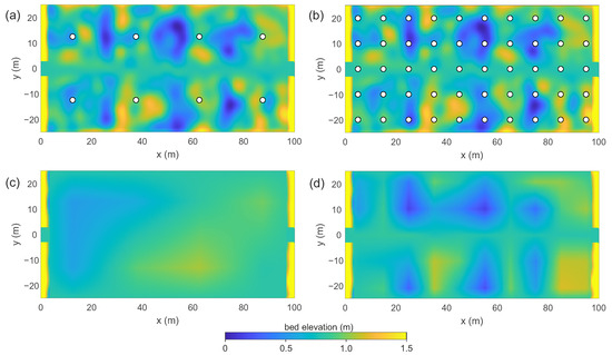
Figure 1.
Examples of coarse-graining of bed elevation fields for a wetland with . Panels (a,b) show sampling grids with and points across the wetland width, corresponding to and sampling points, respectively. Panels (c,d) show the corresponding interpolated bed elevation fields interpolated back onto the computational mesh with m.
For solute transport, boundary conditions were defined as follows: a constant normalized concentration, , was imposed at the inlet; an open (zero-gradient) condition was applied at the outlet; and impermeable, no-flux conditions were enforced along the remaining boundaries.
The governing equations for flow and solute transport were solved using a custom-built two-dimensional finite volume code. The hydrodynamic solver employs the Saint–Venant equations with a second-order time integration scheme, and a Van Leer flux-limited total variation diminishing (TVD) method for spatial advection [26]. For scalar transport, the advection term is handled via the explicit wave-propagation algorithm available in the CLAWPACK library [27,28], while diffusion is treated using the implicit Crank–Nicolson scheme. The computational domain was discretized using a uniform Cartesian grid with 0.5 m resolution. A time step of 1 min was found to ensure numerical stability and convergence of all simulations.
2.5. Bed Topography
Two-dimensional Gaussian random fields of bed elevation, , were generated using a spectral method [29], with given variance , and correlation lengths and in the streamwise (x) and lateral (y) direction, respectively. Note that, in the simulations performed in this study, the variations in free surface elevation are extremely small relative to the mean water depth, and therefore, the variance of bed elevation is, for all practical purposes, the same as the variance of water depth.
In the simulations, we considered three possible values of the normalized standard deviation of bed elevation, , 0.4, and 0.6. For the latter case, we also considered two distinct correlation lengths m and 10 m, corresponding to 0.05 to 0.1 times the longitudinal size of the wetland, L, and 0.1 to 0.2 times the width of the wetland, W. We only considered isotropic fields of bed elevation, for which .
The values chosen for the standard deviation and correlation length were designed to span conditions from nearly flat beds to highly irregular topographies, while still remaining consistent with the assumptions of a depth-averaged shallow-water model. The selected variability in is comparable to that observed in natural wetlands, e.g., [30], where features such as small ridges, depressions, and shallow channels can introduce substantial elevation differences. Considering this range makes it possible to capture a wide variety of plausible wetland morphologies and to derive findings that are relevant for both wetland analysis and design.
For each set of parameter values, we generated 200 random topographies and simulated the flow and mass transport through the wetland. Based on several tests, this was more than sufficient to obtain accurate statistics of the chosen performance metrics that are independent of the number of generated random fields.
2.6. Vegetation Distribution
In the absence of empirical relationships linking vegetation stem density to water depth, simulations with heterogeneous bed topography were conducted assuming a uniform vegetation density of and diameter mm. These values fall within the ranges reported by Valiela et al. [23] for Spartina alterniflora, and they provide representative conditions for emergent wetland vegetation. This approach allows us to isolate the influence of bed variability independently from vegetation heterogeneity.
Complementary simulations considered wetlands with flat beds, and thus a uniform flow depth of m, but heterogeneous vegetation distributions. Random fields of stem density were generated with the same random field generator used for topography, but using an exponential covariance function following [17]. The analysis focused on wetlands with an average stem density , a standard deviation , and a correlation length m. This level of variability is also consistent with reported ranges for the salt marsh grass Spartina alterniflora [23]. For these parameter values, 200 random realizations of vegetation density were generated.
2.7. Resampling Approach
The impact of data resolution on model predictions was assessed by comparing coarsened representations of bed elevation and vegetation density against a high-resolution benchmark. The benchmark corresponds to fields directly defined on the computational mesh used in the simulations, which has a grid size of 0.5 m.
To generate coarsened inputs, the high-resolution fields were resampled on a uniformly spaced square grid with grid size . Since the wetland length L is twice its width W, the spacing was defined as , where is the number of intervals along the width. The first sampling point is placed at a distance from the wetland boundaries, ensuring that the grid is centered in the wetland and that the number of longitudinal nodes is twice the number of lateral ones. The coarsened fields were then linearly interpolated back onto the computational mesh for use in the simulations.
The number of sampling intervals varied between 2 and 100, corresponding to coarsened grid sizes ranging from 25 m to 0.5 m. To enable comparison across different correlation lengths, the results are expressed in terms of the normalized grid size , where is the correlation length of the random field. Accordingly, spans from 0.1 to 5 for m and from 0.05 to 2.5 for m.
Illustrative examples are shown in Figure 1 for a wetland topography with . Figure 1a shows the case , corresponding to sampling points, with the resulting interpolated bed elevation field on the computational mesh shown in Figure 1c. Figure 1b shows the case , corresponding to sampling points, with the interpolated field shown in Figure 1d.
2.8. Error Metrics
To assess the accuracy of the coarse-grained models, we evaluated three characteristic parameters that govern wetland performance. The first parameter is the nominal residence time, , defined as the ratio of wetland water volume V to inflow discharge Q:
This parameter is widely used as the primary design criterion for constructed wetlands, as it ensures that solutes remain in the system long enough for treatment processes to occur [7]. In all high-resolution benchmark simulations, the outlet water level was adjusted so that the nominal residence time is fixed at (see Section 2.4). The relative error in the coarse-grained model is then defined as
where is the value obtained from the coarse-grained model.
The second parameter is the variance of the residence time, , which characterizes the spread of solute travel times. It is obtained by simulating conservative tracer transport at constant inlet concentration. The normalized outlet concentration, , yields the cumulative residence time distribution (RTD), . From its complementary form, , the mean residence time and its variance follow as
In our simulations, , since the solute is conservative and the integration time is sufficiently long to capture the full RTD tail. The variance of residence time is often used as a basis for evaluating hydraulic efficiency metrics [11,31]. The relative error in this parameter is defined as
where is the benchmark (high-resolution) value.
The third parameter is the outlet concentration in reactive transport simulations, , which directly reflects contaminant removal efficiency. Its relative error is defined as
where is the outlet concentration from the benchmark model, and is the inlet concentration. Normalizing by rather than provides a clearer measure of the deviation in predicted treatment performance relative to the influent load.
3. Results
3.1. Flow Patterns
Examples of simulated wetlands with isotropic bathymetry fields are shown in Figure 2, together with streamlines obtained from 100 source points at the inlet. Figure 2a–c represent wetlands with correlation length m and increasing relative standard deviation of bed elevation, , , and , respectively, while Figure 2d shows a wetland with and m. In all cases, the mean water depth is fixed at m.
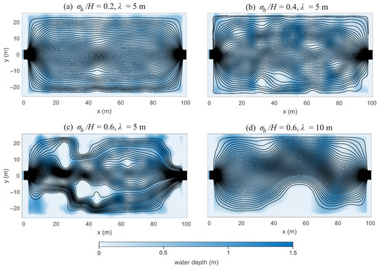
Figure 2.
Examples of simulated wetlands with isotropic random bathymetry fields and corresponding streamlines from 100 inlet source points. Panels (a–c) show increasing relative standard deviation of bed elevation () at fixed correlation length m. Panel (d) shows a case with the same variance as (c) but a larger correlation length ( m). Higher variance promotes the formation of shallow areas, dead zones, and internal dry patches, whereas increasing correlation length reduces small-scale islands and favors larger-scale topographic features.
For m, increasing the variance of bed elevation strongly alters wetland morphology. At low variability (), the wetland resembles a nearly uniform bathymetry, although local differences in depth produce variations in velocity. When , small internal dry patches and bank irregularities appear, slightly deflecting streamlines. At the highest variance (), dry zones coalesce into distinct internal islands, which contract and split the flow into separate pathways. This case highlights how highly variable bathymetry with a relatively small correlation length can generate complex internal flow structures.
The comparison between Figure 2c,d illustrates the role of correlation length. For the same variance (), a larger correlation length ( m) suppresses the formation of small internal islands, while promoting broader lateral features such as bars along the wetland banks.
As increases, the streamlines become increasingly irregular, with enhanced flow divergence and the formation of low-velocity dead zones near bathymetric highs. Overall, wetlands with higher variance in bed elevation exhibit greater hydraulic complexity, while increasing correlation length shifts the morphology from fragmented islands toward larger-scale topographic features.
3.2. Nominal Residence Time
Figure 3 presents the relative error in the nominal residence time, , as a function of the normalized grid size, , for four combinations of bed elevation variability and correlation length. In each panel, the median value across replicate realizations is shown together with the variability range defined by the 16th and 84th percentiles, which are representative of the standard deviation, and 5th and 95th percentiles, which are representative of the extreme values.
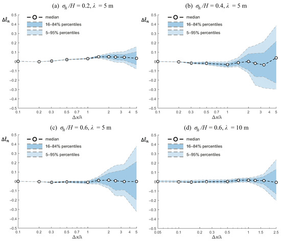
Figure 3.
Relative error in the nominal residence time, , as a function of the normalized grid size, , for wetlands with different bathymetric characteristics. Panels show results for (a) , m; (b) , m; (c) , m; and (d) , m. Symbols indicate the median error across realizations, with shaded bands corresponding to the 16th–84th and 5th–95th percentile ranges.
Overall, the results indicate that, on average, the nominal residence time is relatively insensitive to grid coarsening, with median errors typically within a few percent even when the grid size approaches or exceeds the bathymetric correlation length. For the case with moderate bed variability (, Figure 3a), errors remain small and positive, and the spread across realizations only becomes significant when . Increasing the variance of bed elevation to (Figure 3b) leads to more variable outcomes, with median errors that are slightly negative at intermediate grid sizes and a much wider range of realizations at coarse resolution. A similar pattern is observed for and m (Figure 3c), although the median error remains close to zero and the widening of the distribution is the most prominent effect.
Changing the correlation length alters the error behavior. For and m (Figure 3d), the error distribution is narrow at fine resolutions, but at coarser grids the variability increases (with errors up to for the 90% confidence interval) and both positive and negative outliers appear. Compared to the shorter correlation length case (Figure 3c), the larger reduces the bias in the median error but does not prevent the emergence of large deviations in individual realizations when .
In summary, these results suggest that while the nominal residence time is, on average, robust to grid coarsening, the uncertainty across realizations increases substantially as the grid size becomes larger than the correlation length, particularly for cases with higher bed elevation variance.
3.3. Variance of the Residence Time
Figure 4 shows the relative error in the variance of the residence time, , as a function of the normalized grid size . As in the case of the nominal residence time, the figure reports the median error together with percentile ranges that quantify the variability across realizations. The results indicate that the variance is systematically more sensitive to grid resolution than the nominal residence time, with errors becoming increasingly negative as grows.
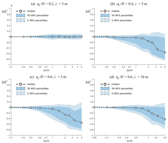
Figure 4.
Relative error in the variance of the residence time, , as a function of the normalized grid size, , for wetlands with different bathymetric characteristics. Panels show results for (a) , m; (b) , m; (c) , m; and (d) , m. Symbols represent the median error across realizations, while shaded bands indicate the 16th–84th and 5th–95th percentile ranges.
For weak bathymetric variability (, Figure 4a), the errors remain small, with the median fluctuating near zero across all grid sizes. Although the spread increases for , the error distribution remains largely centered, suggesting that variance is well preserved under coarse resolution when the bathymetry is relatively uniform.
As bathymetric variability increases, however, a clear trend of underestimation emerges. For (Figure 4b) and (Figure 4c), the median becomes increasingly negative with coarsening grid resolution, indicating that variance is consistently underestimated relative to the high-resolution reference. The spread of errors also widens substantially, with the 5th percentile dropping below for in both cases. This indicates that coarse grids not only bias the variance but also introduce high variability between realizations, reflecting a loss of robustness.
The effect of increasing the correlation length (Figure 4d) slightly mitigates this sensitivity, at least for finer resolutions. For m, the errors remain relatively small for , but as the resolution is degraded, the same pattern of negative bias and broadening distribution reappears. At the coarsest resolution, the median error approach , with extreme values nearly reaching .
Overall, these results highlight that the variance of residence times is far more vulnerable to loss of spatial detail than the nominal residence time. While nominal residence time errors remained relatively small even for coarse grids, variance shows a strong and systematic underestimation, particularly in wetlands with more variable bathymetry and shorter correlation lengths. This indicates that small-scale topographic variability plays a central role in generating dispersive flow paths and controlling residence time variability. When these fine-scale gradients are smoothed through coarse-graining, hydraulic heterogeneity diminishes, leading to a narrower predicted residence time distribution and reduced variance.
3.4. Outlet Concentration
Figure 5 shows the relative error in the predicted outlet concentration, , as a function of the normalized grid size, , across the different wetland scenarios. In contrast to the variance of the residence time, the behavior of is less systematic, reflecting the fact that the outlet concentration is mostly dependent on the nominal residence time, and the uncertainty in is a scaled version of the uncertainty in .
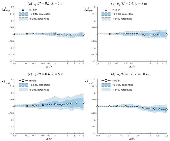
Figure 5.
Relative error in the outlet concentration, , as a function of normalized grid size, , for wetlands with different bathymetric variability and correlation lengths. The results highlight that outlet concentration is less systematically biased by grid resolution than the variance of the residence time (Figure 4), with variations generally limited to a few percentage points. However, the associated uncertainty tends to increase with stronger bathymetric variability and coarser resolution, particularly when the bed elevation field is highly heterogeneous.
For the case of low bathymetric variability (, Figure 5a), the median error remains close to zero for all resolutions, with values fluctuating between slightly positive at finer grids and slightly negative at coarser grids. The spread across realizations, as indicated by the percentile bands, remains relatively narrow, suggesting that predictions of outlet concentration are generally robust when bathymetric variability is small.
As the bathymetric variability increases to (Figure 5b), a modest increase in the dispersion of is observed, especially at larger grid sizes. The median error remains small and does not show a strong systematic bias, although the spread widens, indicating that the reliability of coarse models decreases with increasing bed variability.
For high bathymetric variability (, Figure 5c), the effect of grid coarsening becomes more pronounced. The median error slightly increases with grid size, reaching values on the order of a few percent at , and the uncertainty band broadens considerably. In this case, the results exhibit a slight bias toward overestimating the outlet concentration. These patterns may reflect nonlinear effects of coarse-graining on depth–drag relationships and flow connectivity. However, given the complex, nonlinear interactions between bathymetry, hydraulics, and solute transport, it is difficult to provide a definitive explanation for the observed bias.
Finally, when the correlation length is increased to m while maintaining (Figure 5d), the overall trends remain similar, but the dispersion is somewhat reduced compared to the m case. The median error stays close to zero for fine resolutions and becomes slightly negative at coarse resolutions, while the uncertainty range remains moderate. This suggests that larger correlation lengths mitigate the sensitivity of outlet concentration predictions to grid resolution, even under strong bathymetric variability.
Overall, these results highlight that outlet concentration is less systematically biased by grid resolution than the residence time metrics, but the associated uncertainty can grow with increasing bathymetric variability and coarsening, particularly when the bed elevation field is highly heterogeneous.
3.5. Effect of a Non-Uniform Vegetation Distribution
We now examine the influence of vegetation data resolution on model error in a wetland with a flat bed and non-uniform vegetation distribution. In this configuration, the water depth is uniform, so variations in the nominal residence time are driven solely by the spatial heterogeneity of vegetation. We focus on a single vegetation scenario with an average density of , stem diameter mm, standard deviation of stem density , and spatial correlation length m.
Figure 6 presents an example realization of such a wetland. The figure shows that water depth is essentially uniform, and streamlines are similar to those of a uniform wetland, indicating that the flow patterns are largely unaffected by vegetation heterogeneity at this scale. However, this outcome may not hold if vegetation distributions were to organize into larger-scale structures with reduced stem density along preferential pathways, in which case the flow would likely align with channels of minimum resistance while avoiding regions of higher resistance. This effect could be further amplified in the presence of correlations between bed topography and vegetation density, which, as discussed earlier, are not considered in this study.
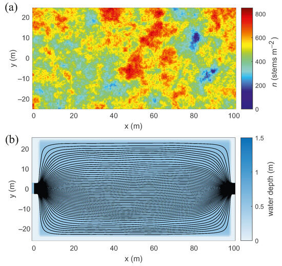
Figure 6.
Example realization of a wetland with a flat bed, average vegetation density of 500 , stem diameter 3 mm, standard deviation of 300 , and spatial correlation length m: (a) vegetation density; (b) water depth and streamlines. The figure shows uniform water depth and streamlines, illustrating that flow patterns are largely unaffected by vegetation heterogeneity at this scale.
Figure 7 quantifies the effect of vegetation data resolution on model error. Figure 7a shows the relative error in the variance of the residence time, , as a function of the normalized grid size, . The median error is small for fine resolutions (), but both the median and variability increase at coarser resolutions, reflecting greater uncertainty in predicting residence time variance when vegetation heterogeneity is coarsely represented.
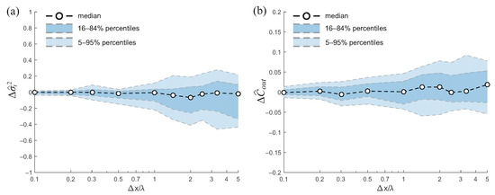
Figure 7.
Model error as a function of normalized grid size for a wetland with a flat bed and heterogeneous vegetation (average density , stem diameter 3 mm, standard deviation , m). Panel (a) shows the error in the variance of the residence time, , while panel (b) shows the error in the output concentration, . Coarse-graining the vegetation field slightly increases uncertainty in residence time and outlet concentration, but the relative error in solute removal remains mostly within 5%, indicating robustness of model predictions to vegetation resolution under the conditions considered.
Figure 7b reports the error in the outlet concentration, . In this case, errors remain relatively small across the range of resolutions, with median values close to zero. The variability increases modestly for coarser grids, but the overall magnitude of the error is limited.
In summary, while coarse-graining the vegetation field introduces some variability in the predicted residence time and a minor increase in uncertainty for outlet concentration, the effect on solute removal is limited, indicating that the model is relatively robust to the resolution of vegetation data for the conditions considered.
4. Discussion
The results show that the spatial resolution of topographic input data has a clear but selective influence on modeled wetland hydraulics. Coarse-graining the bathymetry primarily reduced small-scale variability in flow organization, reflected in a systematic underestimation of residence-time variance. This occurs because finer topographic details, such as small depressions and ridges, create localized storage zones and tortuous flow paths that enhance hydraulic dispersion. When these features are smoothed out, the model predicts more uniform velocities and narrower residence-time distributions. However, this simplification did not proportionally degrade treatment performance: the outlet concentration was relatively insensitive to the loss of topographic detail, remaining closely tied to the nominal residence time. This finding indicates that small-scale heterogeneity mainly affects intra-wetland transport dynamics rather than the overall treatment efficiency under the steady, idealized flow conditions examined here. Comparable sensitivity to bathymetric smoothing has been observed in ecological wetland models, where topographic roughness determines the persistence and extent of shallow-water habitats [32].
Vegetation heterogeneity played a comparatively minor role at small scales. Within the tested range of stem density variability, spatial patterns in vegetation resistance had limited impact on residence-time metrics or outlet concentrations. While local flow deviations occurred around patches of denser vegetation, these effects largely averaged out at the system scale. This suggests that, in shallow wetlands with moderate vegetation variability, the hydraulic influence of vegetation structure may be subordinate to that of bed topography. Nevertheless, in natural wetlands where vegetation forms large-scale patches, corridors, or main flow channels, its role in shaping preferential flow paths can be far more significant. For example, Savickis et al. [33] showed that a main flow channel with lower vegetation density induces short-circuiting and reduces hydraulic efficiency, while channel sinuosity and the arrangement of lateral vegetated zones can mitigate these effects. Similarly, Sabokrouhiyeh et al. [17] demonstrated that large, aligned vegetation patches promote preferential flow paths and affect contaminant removal, whereas alternating stem density perpendicular to the flow enhances mixing. These findings highlight that the hydraulic impact of vegetation is scale-dependent, and large-scale spatial organization can substantially influence intra-wetland transport dynamics, warranting targeted investigation.
The interpretation that treatment efficiency is less sensitive to small-scale spatial detail aligns with findings from field and modeling studies emphasizing the dominant role of bulk hydraulic behavior [11,34,35]. For example, in full-scale vegetated cells of surface-flow constructed wetlands, Dykes et al. [35] found that hydraulic inefficiencies were primarily driven by large-scale design factors, such as cell geometry, inlet–outlet configuration, and hydraulic loading, while sub-meter vegetation heterogeneity had comparatively little impact on treatment performance. Instead, vegetation influenced removal primarily through seasonal growth and climatic variability rather than fine-scale spatial variability. Sabokrouhiyeh et al. [11] further demonstrated that, above a threshold stem density typical of treatment wetlands (≈), hydraulic performance metrics were largely insensitive to the exact value of vegetation density, supporting the notion that fine-scale vegetation details are secondary for overall hydraulic efficiency. Similarly, Guzman et al. [36] and Persson [37] observed that wetland topographies with islands or deep zones modify circulation, primarily by altering major flow paths rather than by small-scale surface roughness. Brovelli et al. [38] further demonstrated that hydraulic conductivity heterogeneity at scales comparable to the system geometry strongly affects residence-time distributions, reinforcing that model sensitivity depends on the relative scale of spatial variability to overall system size.
From a modeling perspective, these results imply that moderate coarsening of topographic or vegetation data can be acceptable when predicting bulk hydraulic or treatment metrics, provided the grid spacing remains smaller than the dominant correlation length of the bed features. In contrast, metrics that depend on detailed mixing behavior, such as residence time variance or short-circuiting indices, require finer spatial resolution. This scale dependence mirrors similar findings in hydraulic modeling of wetlands and river systems (e.g., [39,40,41]), where predictive accuracy deteriorates once the grid size exceeds key spatial correlation scales.
Future research should extend these analyses to explore how resolution effects interact with additional physical processes. Varying discharge conditions, submerged vegetation, or seasonally variable canopy structures could reveal nonlinear sensitivities absent under steady, uniform forcing. Coupling between topography and vegetation distribution (common in real wetlands) may also alter flow organization in ways not captured by the present approach. Incorporating such feedback in three-dimensional frameworks or field-validated models would help generalize the conclusions to more complex, natural systems.
5. Conclusions
This study examined the effect of the spatial resolution of bathymetric and vegetation data on the prediction of residence time and solute treatment in shallow-water wetlands. Using synthetic wetlands with spatially correlated random fields for bed elevation and vegetation density, we quantified how coarse-graining the input data impacts model outputs. The median error in nominal residence time was generally small, although its variability across realizations increased with larger topographic heterogeneity. The variance of residence time was the most sensitive metric, exhibiting a tendency to be underestimated as the grid size increased. In contrast, errors in outlet concentration remained relatively small (<5%) even for grid sizes up to 1–5 times the correlation length of the bed features, suggesting that outlet concentration is more strongly correlated with nominal residence time than with its variance.
For the range of vegetation stem density variability considered here, coarse-graining vegetation patterns had a less significant impact on both residence time metrics and outlet concentration compared to bathymetry. This result, however, may not hold if vegetation were organized into larger-scale structures with preferential low-density pathways, which would likely channel flow along paths of minimum resistance. Such configurations were not considered in this study.
A few important limitations should be noted. The results presented in this study were obtained under the assumption of uniform vegetation stem density and diameter across the wetland. The potential interaction between vegetation density and water depth, which was not explored here, represents an important direction for future research. In natural systems, vegetation structure and bed topography often covary, as vegetation tends to establish preferentially in zones of specific depth or flow conditions. Such spatial coupling can modify the local hydraulic resistance and feedback on flow organization, potentially amplifying or dampening the resolution effects observed in this study. For instance, correlations between elevated areas and sparse vegetation might enhance short-circuiting at coarse resolution, whereas vegetation concentrated in depressions could counteract flow acceleration by increasing resistance. Exploring these coupled effects would provide a more realistic understanding of how spatial heterogeneity influences model sensitivity to input resolution.
Moreover, the use of shallow-water and depth-averaged solute transport models, while computationally efficient, relies on a few simplifying assumptions. Vertical variations in flow and solute concentration are neglected, which may reduce accuracy in systems with strong stratification, highly heterogeneous vegetation, or vertical gradients at the inlet. As a result, the findings presented here should be interpreted within the limits of two-dimensional, depth-averaged dynamics, and caution should be exercised when extrapolating to wetlands where three-dimensional circulation or vertical mixing processes play a dominant role. These limitations should be considered when interpreting the results, especially for more complex or heterogeneous wetland systems.
Overall, this work provides a quantitative framework for assessing how input data resolution affects the reliability of shallow-water wetland models and identifies conditions under which coarse-graining may be acceptable, offering guidance for both field measurements and numerical modeling. In practical terms, the results suggest that when the grid spacing or survey resolution is smaller than roughly half the dominant correlation length of bed topography, errors in hydraulic and treatment metrics remain within a few percent. Beyond this threshold, uncertainty increases rapidly, particularly in wetlands with highly variable microtopography. These findings therefore provide a basis for selecting appropriate grid resolutions or survey intervals according to the expected spatial heterogeneity of the site.
Author Contributions
Conceptualization, A.B.-B. and A.M.; methodology, A.B.-B. and A.M.; software, A.B.-B.; formal analysis, A.B.-B. and E.D.; resources, A.M. and A.B.-B.; writing—original draft preparation, A.B.-B.; writing—review and editing, E.D., A.M., G.S. and A.B.-B.; visualization, A.B.-B.; project administration, A.M., A.B.-B. and G.S.; funding acquisition, A.M. and A.B.-B. All authors have read and agreed to the published version of the manuscript.
Funding
This study was carried out within the RETURN Extended Partnership and received funding from the European Union Next-GenerationEU (National Recovery and Resilience Plan—NRRP, Mission 4, Component 2, Investment 1.3—D.D. 1243 2/8/2022, PE0000005, CUP C93C22005160002).
Data Availability Statement
This study relies entirely on data generated by the mathematical models described in the paper. Further inquiries can be directed to the corresponding authors.
Conflicts of Interest
The authors declare no conflicts of interest.
References
- Vymazal, J. Constructed wetlands for treatment of industrial wastewaters: A review. Ecol. Eng. 2014, 73, 724–751. [Google Scholar] [CrossRef]
- Katsenovich, Y.P.; Hummel-Batista, A.; Ravinet, A.J.; Miller, J.F. Performance evaluation of constructed wetlands in a tropical region. Ecol. Eng. 2009, 35, 1529–1537. [Google Scholar] [CrossRef]
- Cheng, Y.; Stieglitz, M.; Turk, G.; Engel, V. Effects of anisotropy on pattern formation in wetland ecosystems. Geophys. Res. Lett. 2011, 38, L04402. [Google Scholar] [CrossRef]
- Arheimer, B.; Wittgren, H.B. Modelling nitrogen removal in potential wetlands at the catchment scale. Ecol. Eng. 2002, 19, 63–80. [Google Scholar] [CrossRef]
- Meng, P.; Pei, H.; Hu, W.; Shao, Y.; Li, Z. How to increase microbial degradation in constructed wetlands: Influencing factors and improvement measures. Bioresour. Technol. 2014, 157, 316–326. [Google Scholar] [CrossRef]
- Thackston, E.L.; Shields, F.D.; Schroeder, P.R. Residence Time Distributions of Shallow Basins. J. Environ. Eng. 1987, 113, 1319–1332. [Google Scholar] [CrossRef]
- Kadlec, R.H.; Wallace, S. Treatment Wetlands, 2nd ed.; CRC Press: Boca Raton, FL, USA, 2008. [Google Scholar] [CrossRef]
- Zhao, F.; Zhang, X.; Xu, Z.; Feng, C.; Pan, W.; Lu, L.; Luo, W. Review of hydraulic conditions optimization for constructed wetlands. J. Environ. Manag. 2024, 370, 122377. [Google Scholar] [CrossRef]
- Carleton, J.N.; Grizzard, T.J.; Godrej, A.N.; Post, H.E. Factors affecting the performance of stormwater treatment wetlands. Water Res. 2001, 35, 1552–1562. [Google Scholar] [CrossRef]
- Holland, J.F.; Martin, J.F.; Granata, T.; Bouchard, V.; Quigley, M.; Brown, L. Effects of wetland depth and flow rate on residence time distribution characteristics. Ecol. Eng. 2004, 23, 189–203. [Google Scholar] [CrossRef]
- Sabokrouhiyeh, N.; Bottacin-Busolin, A.; Savickis, J.; Nepf, H.; Marion, A. A numerical study of the effect of wetland shape and inlet-outlet configuration on wetland performance. Ecol. Eng. 2017, 105, 170–179. [Google Scholar] [CrossRef]
- Diamond, J.S.; McLaughlin, D.L.; Slesak, R.A.; Stovall, A. Microtopography is a fundamental organizing structure of vegetation and soil chemistry in black ash wetlands. Biogeosciences 2020, 17, 901–915. [Google Scholar] [CrossRef]
- Zheng, L.; Wang, X.; Li, D.; Xu, G.; Guo, Y. Spatial heterogeneity of vegetation extent and the response to water level fluctuations and micro-topography in Poyang Lake, China. Ecol. Indic. 2021, 124, 107420. [Google Scholar] [CrossRef]
- Keiser, A.D.; Davis, C.L.; Smith, M.; Bell, S.L.; Hobbie, E.A.; Hofmockel, K.S. Depth and microtopography influence microbial biogeochemical processes in a forested peatland. Plant Soil 2024, 509, 833–846. [Google Scholar] [CrossRef]
- Harvey, J.; Choi, J.; Wilcox, W.; Brown, M.; Lal, W. Biophysical simulation of wetland surface water flow to predict changing water availability in the Everglades. Ecol. Eng. 2025, 212, 107491. [Google Scholar] [CrossRef]
- Lightbody, A.F.; Nepf, H.M.; Bays, J.S. Modeling the hydraulic effect of transverse deep zones on the performance of short-circuiting constructed treatment wetlands. Ecol. Eng. 2009, 35, 754–768. [Google Scholar] [CrossRef]
- Sabokrouhiyeh, N.; Bottacin-Busolin, A.; Tregnaghi, M.; Nepf, H.; Marion, A. Variation in contaminant removal efficiency in free-water surface wetlands with heterogeneous vegetation density. Ecol. Eng. 2020, 143, 105662. [Google Scholar] [CrossRef]
- Bottacin-Busolin, A.; Santovito, G.; Marion, A. Model insights into the role of bed topography on wetland performance. Water 2025, 17, 2528. [Google Scholar] [CrossRef]
- Jarihani, A.A.; Callow, J.N.; McVicar, T.R.; Van Niel, T.G.; Larsen, J.R. Satellite-derived Digital Elevation Model (DEM) selection, preparation and correction for hydrodynamic modelling in large, low-gradient and data-sparse catchments. J. Hydrol. 2015, 524, 489–506. [Google Scholar] [CrossRef]
- Seenath, A. Effects of DEM resolution on modeling coastal flood vulnerability. Mar. Geod. 2018, 41, 581–604. [Google Scholar] [CrossRef]
- Wu, W. Computational River Dynamics, 1st ed.; CRC Press: London, UK, 2007. [Google Scholar] [CrossRef]
- Chow, V.T. Open-Channel Hydraulics; McGraw-Hill Book Co.: New York, NY, USA, 1959. [Google Scholar]
- Valiela, I.; Teal, J.M.; Deuser, W.G. The nature of growth forms in the salt marsh grass spartina alterniflora. Am. Nat. 1978, 112, 461–470. [Google Scholar] [CrossRef]
- Hudon, C. Shift in wetland plant composition and biomass following low-level episodes in the St. Lawrence River: Looking into the future. Can. J. Fish. Aquat. Sci. 2004, 61, 603–617. [Google Scholar] [CrossRef]
- Serra, T.; Fernando, H.J.S.; Rodrìguez, R.V. Effects of emergent vegetation on lateral diffusion in wetlands. Water Res. 2004, 38, 139–147. [Google Scholar] [CrossRef]
- Van Leer, B. Towards the ultimate conservative difference scheme. II. Monotonicity and conservation combined in a second-order scheme. J. Comput. Phys. 1974, 14, 361–370. [Google Scholar] [CrossRef]
- LeVeque, R.J. Wave propagation algorithms for multidimensional hyperbolic systems. J. Comput. Phys. 1997, 131, 327–353. [Google Scholar] [CrossRef]
- Calhoun, D.; LeVeque, R.J. A cartesian grid finite-volume method for the advection-diffusion equation in irregular geometries. J. Comput. Phys. 2000, 157, 143–180. [Google Scholar] [CrossRef]
- Lang, A.; Potthoff, J. Fast simulation of Gaussian random fields. Monte Carlo Methods Appl. 2011, 17, 195–214. [Google Scholar] [CrossRef]
- Price, J.S. Water level regimes in prairie sloughs. Can. Water Resour. J. 1993, 18, 95–106. [Google Scholar] [CrossRef]
- Persson, J.; Somes, N.L.G.; Wong, T.H.F. Hydraulics efficiency of constructed wetlands and ponds. Water Sci. Technol. 1999, 40, 291–300. [Google Scholar] [CrossRef]
- Schaffer-Smith, D.; Swenson, J.J.; Reiter, M.E.; Isola, J.E. Quantifying shorebird habitat in managed wetlands by modeling shallow water depth dynamics. Ecol. Appl. 2018, 28, 1534–1545. [Google Scholar] [CrossRef]
- Savickis, J.; Bottacin-Busolin, A.; Zaramella, M.; Sabokrouhiyeh, N.; Marion, A. Effect of a meandering channel on wetland performance. J. Hydrol. 2016, 535, 204–210. [Google Scholar] [CrossRef]
- Wörman, A.; Kronnäs, V. Effect of pond shape and vegetation heterogeneity on flow and treatment performance of constructed wetlands. J. Hydrol. 2005, 301, 123–138. [Google Scholar] [CrossRef]
- Dykes, C.; Pearson, J.; Bending, G.D.; Abolfathi, S. Hydraulic efficiency and mixing dynamics in surface flow constructed wetlands: Influence of design, vegetation phenology, and climate variability. Water Res. 2025, 285, 124110. [Google Scholar] [CrossRef] [PubMed]
- Guzman, C.B.; Cohen, S.; Xavier, M.; Swingle, T.; Qiu, W.; Nepf, H. Island topographies to reduce short-circuiting in stormwater detention ponds and treatment wetlands. Ecol. Eng. 2018, 117, 182–193. [Google Scholar] [CrossRef]
- Persson, J. Improving wetland design. Water 2005, 21, 52. [Google Scholar]
- Brovelli, A.; Carranza-Diaz, O.; Rossi, L.; Barry, D. Design methodology accounting for the effects of porous medium heterogeneity on hydraulic residence time and biodegradation in horizontal subsurface flow constructed wetlands. Ecol. Eng. 2011, 37, 758–770. [Google Scholar] [CrossRef]
- O’Sullivan, A.M.; Devito, K.J.; Ogilvie, J.; Linnansaari, T.; Pronk, T.; Allard, S.; Curry, R.A. Effects of topographic resolution and geologic setting on spatial statistical river temperature models. Water Resour. Res. 2020, 56, e2020WR028122. [Google Scholar] [CrossRef]
- Hou, J.; Li, X.; Pan, Z.; Wang, J.; Wang, R. Effect of digital elevation model spatial resolution on depression storage. Hydrol. Processes 2021, 35, e14381. [Google Scholar] [CrossRef]
- Zhang, X.; Wright, K.; Passalacqua, P.; Simard, M.; Fagherazzi, S. Improving channel hydrological connectivity in coastal hydrodynamic models with remotely sensed channel networks. J. Geophys. Res. Earth Surf. 2022, 127, e2021JF006294. [Google Scholar] [CrossRef]


Disclaimer/Publisher’s Note: The statements, opinions and data contained in all publications are solely those of the individual author(s) and contributor(s) and not of MDPI and/or the editor(s). MDPI and/or the editor(s) disclaim responsibility for any injury to people or property resulting from any ideas, methods, instructions or products referred to in the content. |
© 2025 by the authors. Licensee MDPI, Basel, Switzerland. This article is an open access article distributed under the terms and conditions of the Creative Commons Attribution (CC BY) license (https://creativecommons.org/licenses/by/4.0/).