You are currently viewing a new version of our website. To view the old version click .
Water
  • Article
  • Open Access

5 November 2025

Deciphering Relative Sea-Level Change in Chesapeake Bay: Impact of Global Mean, Regional Variation, and Local Land Subsidence, Part 1: Methodology

and
Department of Civil & Environmental Engineering, Morgan State University, Baltimore, MD 21251, USA
*
Author to whom correspondence should be addressed.
This article belongs to the Special Issue Climate Risk Management, Sea Level Rise and Coastal Impacts

Abstract

The Chesapeake Bay (CB) region faces significant risks from relative sea-level change (RSLC), driven by global mean sea-level rise (GMSLR), regional sea-level rise (RSLR), and local land subsidence (LS). This study introduces a methodology to decipher RSLC trends in the CB area by integrating these components. We develop trend equations spanning 1900–2100, incorporating acceleration for GMSLR and RSLR since 1992, with linear LS estimation using tide gauge, satellite altimetry, and InSAR data. Our approach employs dynamic RSLC equations, Maclaurin series expansions, and inverse simulations to project RSLC trends through 2100. Stable RSLC rates require over 122 years of data for reliable linear trend estimation, with the Baltimore tide gauge providing the necessary long-term dataset. Similarity in monthly mean sea-level variations within a coastal region enables a new method to identify LS from short-term tide gauge data by correlating it with corresponding long-term data at Baltimore. LS is categorized into bedrock-surface subsidence (BSS) and compaction subsidence (CS), with methods proposed to map BSS contours and estimate CS. CS is further classified into primary consolidation, secondary consolidation, construction-induced, and negative subsidence to determine specific compaction types. The projection model highlights the dominant influence of GMSLR acceleration since 1992, with local LS and RSLR influenced by ocean circulation, density changes, and gravitational, rotational, and deformational (GRD) effects. This integrated approach enhances understanding and predictive reliability for RSLC trends, supporting resilience planning and infrastructure adaptation in coastal CB communities.

1. Introduction

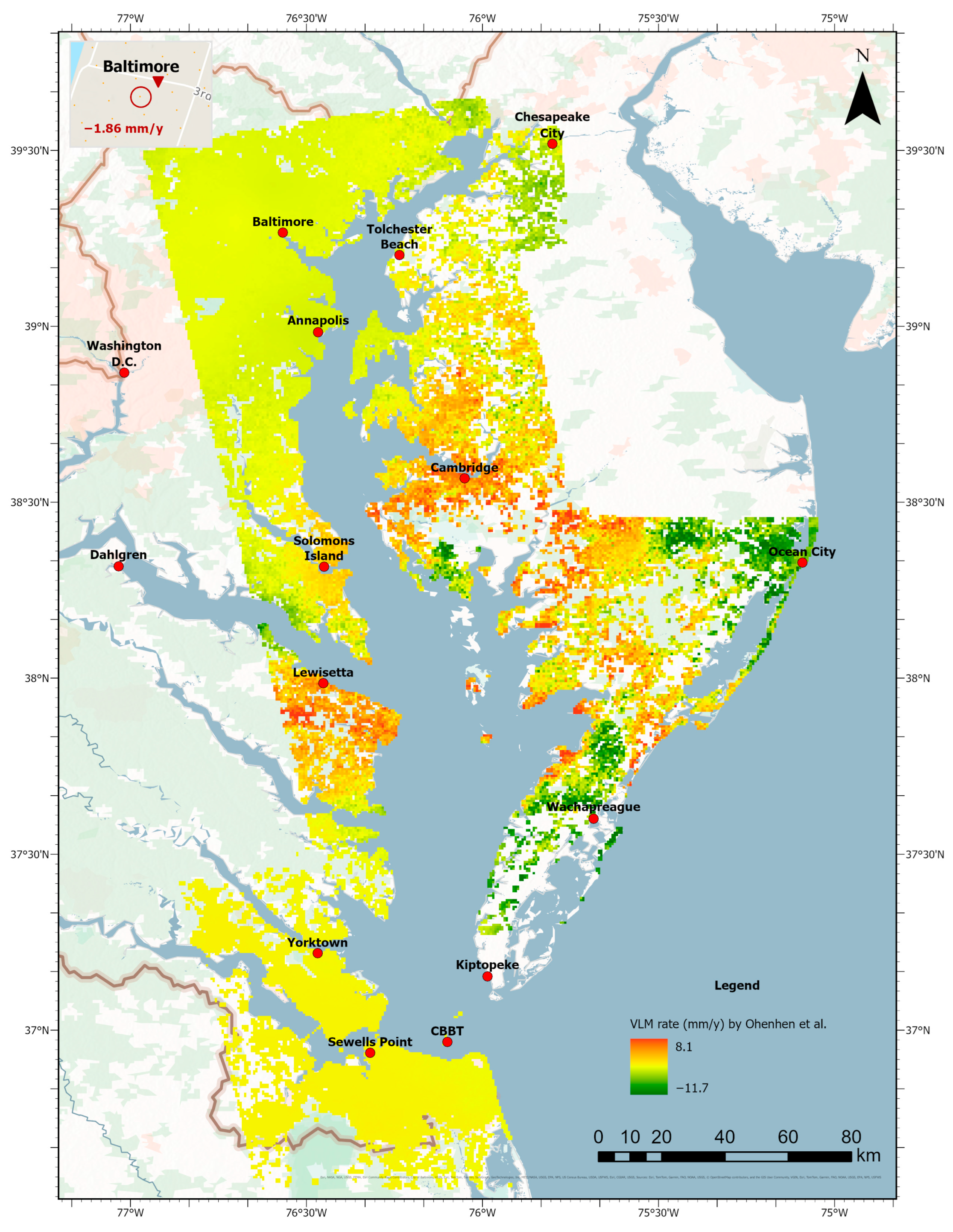
Chesapeake Bay (CB), located in the Mid-Atlantic region, is the largest estuary in the U.S. []. The CB coastal region, spanning across Maryland and Virginia, is at risk of rising sea levels and land subsidence (LS) []. Relative sea level rises 3.24 to 6.04 mm/year at 15 tide gauges (TGs) in Figure 1 along the CB coast []. The projections for mean sea level (MSL) at Baltimore, MD, between 2000 and 2050 suggest a likely relative rise of 22 to 54 cm, with an average of 36 cm [], consistent with Ezer’s (2023) estimate of 31 cm []. These figures underscore the critical concern of relative sea-level change (RSLC) for coastal regions, especially in areas like CB, where complex interactions among global, regional, and local processes drive significant variations in sea-level trends. These variations affect coastal infrastructure, ecosystems, and the livelihoods of communities in the region. Understanding the three processes of RSLC is essential for accurate projections and the development of effective adaptation strategies.
Global mean sea-level rise (GMSLR) is a well-documented phenomenon driven by thermal expansion of seawater and the melting of land-based ice []. Recent studies, such as those by [,,,,,,,,], have provided critical insights into the acceleration and variability of GMSLR, emphasizing the importance of long-term altimetry data for quantifying these trends. While GMSLR establishes a global baseline, regional sea-level rise (RSLR) introduces significant deviations due to factors such as ocean dynamics, gravitational redistribution, sea floor deformation, and the inverse barometer effect (Gregory et al., 2019) []. These regional factors create spatial variability that necessitates localized analysis for regions like Chesapeake Bay.
Chesapeake Bay, in particular, faces additional challenges from LS [], a phenomenon caused by both geological and anthropogenic processes. The interplay of glacial isostatic adjustment (GIA) [] with human-induced activities such as groundwater withdrawal and urban development exacerbates the rate of RSLC in the region [,,,]. Our advances in subsidence categorization—differentiating bedrock-surface subsidence (BSS) from compaction subsidence (CS) and further dissecting CS into primary consolidation, secondary consolidation (PCS), construction-induced (CIS), and negative subsidence (NS)—provide new opportunities to refine RSLC analysis.
Despite significant progress, existing models often treat GMSLR, RSLR, and LS as separate entities, leading to limitations in predictive accuracy. Integrated methodologies, such as those proposed by Parris et al. (2012) [] and refined by our approach, offer a unified framework to simulate and project RSLC by incorporating global, regional, and local contributions. These advancements are particularly valuable for Chesapeake Bay, which serves as a testbed due to its unique geological setting and anthropogenic pressures, and is broadly applicable to other coastal regions with differing geological conditions.
In this paper, Part 1 introduces a novel methodology for deciphering RSLC in Chesapeake Bay, addressing gaps in previous research by integrating comprehensive analyses of GMSLR, RSLR, and LS. The methodology builds on established frameworks, such as the RSLC equation by Gregory et al. (2019) [] and the acceleration model by Parris et al. (2012) [], while introducing new approaches to LS rate estimation at both long-term and short-term tide gauge locations. By applying these innovations to CB in Part 2, this work aims to enhance the understanding of RSLC dynamics and provide a robust foundation for future resilience planning in CB.
Figure 1. Fifteen tide gauges in the Chesapeake Bay area and LS of 1.86 mm/year (denoted as y in figures and tables) at tide gauge Baltimore, MD, detected from InSAR image data [].

2. Definition of Regional Sea-Level Rise (RSLR or h )

This section establishes a general equation of RSLC Δ R at an ocean site in terms of “global-mean sea-level rise” (GMSLR) h [], RSLR h , and vertical land motion (VLM) Δ F —or land subsidence (LS) ( Δ F )—by introducing and defining h to support analysis and simulation of tide-gauge-derived sea-level trends in the next section.
RSLC Δ R in terms of geocentric sea-level change (GSLC) and VLM Δ F : Terminology for sea-level change defined by Gregory et al. [] is employed in this paper as shown in Figure 2 to define RSLC Δ R . Mean sea level (MSL) η is located by its geodetic height η above the reference ellipsoid (a negative value if below). Monthly mean relative sea-level data are used in this research. Sea floor F is the lower boundary of the ocean, its interface with solid earth. The sea floor F is the part of the surface of solid earth (whether bedrock or consolidated sediment, and lying beneath any unconsolidated sediment, e.g., []) that is always or sometimes submerged under sea water. Sea floor change Δ F , also equally referred to as vertical land motion (VLM) Δ F or land subsidence (LS) ( Δ F ), occurs due to glacial isostatic adjustment (GIA), tectonics, sediment compaction, groundwater and fossil fuel withdrawals, and other non-climatic factors []. VLM Δ F and LS ( Δ F ) are used interchangeably to describe sea floor change Δ F , but LS ( Δ F ) is employed more frequently than VLM, especially when describing methodological approaches in this two-part paper. This preference is due to the widespread use of VLM and LS in the literature.
Figure 2. Relationship between surfaces relating to sea level (from []). The normal to the reference ellipsoid defines the vertical in the terrestrial reference frame. The normal to the geoid is the vertical coordinate ( z ) for geophysical fluid dynamics and is anti-parallel to the local effective acceleration g due to gravity. The difference between these two definitions of the vertical direction is greatly exaggerated in this diagram; it is negligible in reality. The local vertical coordinates of mean sea level η , the geoid G , and the sea floor F are relative to the reference ellipsoid, while dynamic sea level ζ ~ is relative to the geoid. The local time–mean thickness of the ocean H is the vertical distance between mean sea level and the sea floor. The deviation of atmospheric pressure p a from its global mean causes the depression B in sea level by the inverse barometer effect.
The change in local mean sea level with respect to the terrestrial reference frame is called geocentric sea-level change (GSLC, Δ η ). Both the mean sea level η and the sea floor height F may change and thus alter relative sea level at an ocean point of interest. Hence, RSLC Δ R [] is geodetically expressed as
Δ R = Δ η Δ F
This means RSLC Δ R represents the difference between GSLC Δ η and VLM Δ F , i.e., RSLC Δ R at any ocean point of interest is the combination of GSLC Δ η and LS ( Δ F ). Gregory et al. (2019) [] further relate RSLC Δ R changes in seawater thickness Δ H :
Δ R = Δ H
GMSLR h : GMSLR can be simply understood as the global mean increase in seawater thickness. The increase Δ V in the ocean volume divided by the ocean surface area A is termed “global-mean sea-level rise” (GMSLR) h []. By definition, GMSLR h is expressed as follows:
h = Δ V A = 1 A Δ η F d A = 1 A Δ R d A = 1 A Δ H d A
Over long, multidecadal to centennial timescales, the primary drivers of GMSLR are thermal expansion due to the heating of the ocean and the addition of water mass associated with ice mass loss from ice sheets and glaciers [,]. Other drivers, such as the movement of water between ocean and land (e.g., groundwater depletion and water impoundment), have a secondary impact on GMSLR, although they can become more significant over certain time periods [].
RSLR h —a local deviation of GMSLR h : However, GSLC Δ η is not uniform across the globe []. At the regional level, GSLC Δ η can deviate significantly from GMSLR h [,,,,,,]. To consider this deviation, we first introduce GSLC Δ η as the combination of GMSLR h and a deviation h of GMSLR h at any specific ocean point of interest. Thus, we can write
h = 1 A Δ h + h F d A = 1 A Δ h d A + 1 A Δ h F d A
This simplifies to
h = h + 1 A Δ h F d A
The global mean of the deviation h must be equal to the global mean of VLM Δ F , i.e., 1 / A Δ h d A = 1 / A Δ F d A . This is required by Equation (5) as follows:
1 A Δ h F d A = 0
This implies that the global mean of the combination of the deviation h and LS (− Δ F ) is zero, i.e., RSLR and VLM do not contribute to GMSLR h . However, both contribute to GSLC Δ η by affecting local seawater thickness Δ H in Equation (3).
Physical understanding of RSLR h : According to [] as shown in Figure 3, the deviation h can be described as
h = Δ ζ Δ B + Δ F + Δ Γ
where Δ ζ represents change in ocean dynamic sea level (as shown Figure 2), Δ B represents the depression in sea level by the inverse barometer effect, and Δ Γ represents the GRD-induced RSLC.
Figure 3. Schematic of relationships between sea-level change components [modified from [] with Δ η = h + h ]. The lengths of the arrows do not have any significance—they are only illustrative—and the dotted horizontal lines serve only to indicate alignment. All of the quantities are differences between two states, and all except h , h θ , and h b are functions of two-dimensional geographical location, specified by latitude and longitude. Any closed circuit gives equality, in which a term has a positive sign when traversed in the direction of its arrow and a negative sign if in the opposite direction to its arrow. For example, Δ R Δ η + Δ F = 0 is the circuit marked in red, Δ ζ = Δ η + Δ B Δ G in orange, Δ Z = Δ ζ + h θ in blue, Δ R + Δ B = Δ Z + h b + Δ Γ in green, and Δ Γ = Δ G Δ F (see Equation (A1)) []. Additionally, RSLR h can be inferred from the following relationships: h = Δ ζ   Δ B + Δ F + Δ Γ , derived from Δ ζ = Δ η + Δ B Δ G , Δ G = Δ F + Δ Γ + h , and Δ η = h + h . [Notes: SLC: sea-level change; IB: inverse barometer; RSLR: regional sea-level rise; GMSLR: global-mean sea-level rise; VLM: vertical land motion (negative land subsidence, LS); GRD: changes in Earth’s gravity, Earth’s rotation (and hence centrifugal acceleration) and viscoelastic solid-Earth deformation].
In this paper, h is referred to as regional sea-level rise (RSLR). In a region like Chesapeake Bay, its variation is generally insignificant. Therefore, we define GSLC Δ η at any specific ocean point of interest as the combination of GMSLR h and RSLR h , a deviation of h , in that region.
Δ η = h + h
We think the regional deviation h resulted from two main factors: (1) regional variations in the ocean’s circulation (currents) and its density (temperature and salinity) [,]; and (2) regional effects of global gravitational, rotational, and deformational (GRD; see Appendix A) changes due to contemporary ice mass loss and the movement of water between land and ocean []. Changes in Earth’s GRD responses dictate the spatial distribution of water across the global ocean [,,,].
RSLR h equation at a tide gauge: Combing Equations (1) and (8), we can estimate h from Δ R at a tide gauge as
h = Δ R h + Δ F
And Δ R can be addressed in terms of h , h , and Δ F as
Δ R = h + h Δ F
This quantity, RSLR h is defined throughout the ocean with Equation (9), providing a representation of the combined regional contribution to local RSLC Δ R in Equation (10) in a region such as the Chesapeake Bay area. Equations (8)–(10) clarify that the RSLR term h causes the local GSLC at a tide gauge Δ η to differ from GMSLR h .

3. Trend Equations of RSLC

In Section 3, we further develop RSLC trend equations based on the general dynamic RSLC Equation (10) established in Section 2. These equations are then used to analyze, simulate, and project RSLC from tide gauge data and to separate the RSLC trend into its components: GMSLR, RSLR, and LS.
General trend equation of RSLC with RSLR, GMSLR, and local LS: Let η ¯ , F ¯ , and R ¯ denote trends of dynamic GSLC Δ η , VLM Δ F , and RSLC Δ R , respectively. Additionally, let h ¯ and h ¯ denote trends of dynamic h and h , respectively. The RSLR Δ R is based on monthly mean sea-level data. Both η ¯ , and F ¯ change with time t in years.
A general trend equation of RSLC derived from dynamic RSLC Equation (10) and GSLC Equation (8) is the following:
R ¯ = η ¯ F ¯ = h ¯ + h ¯ F ¯
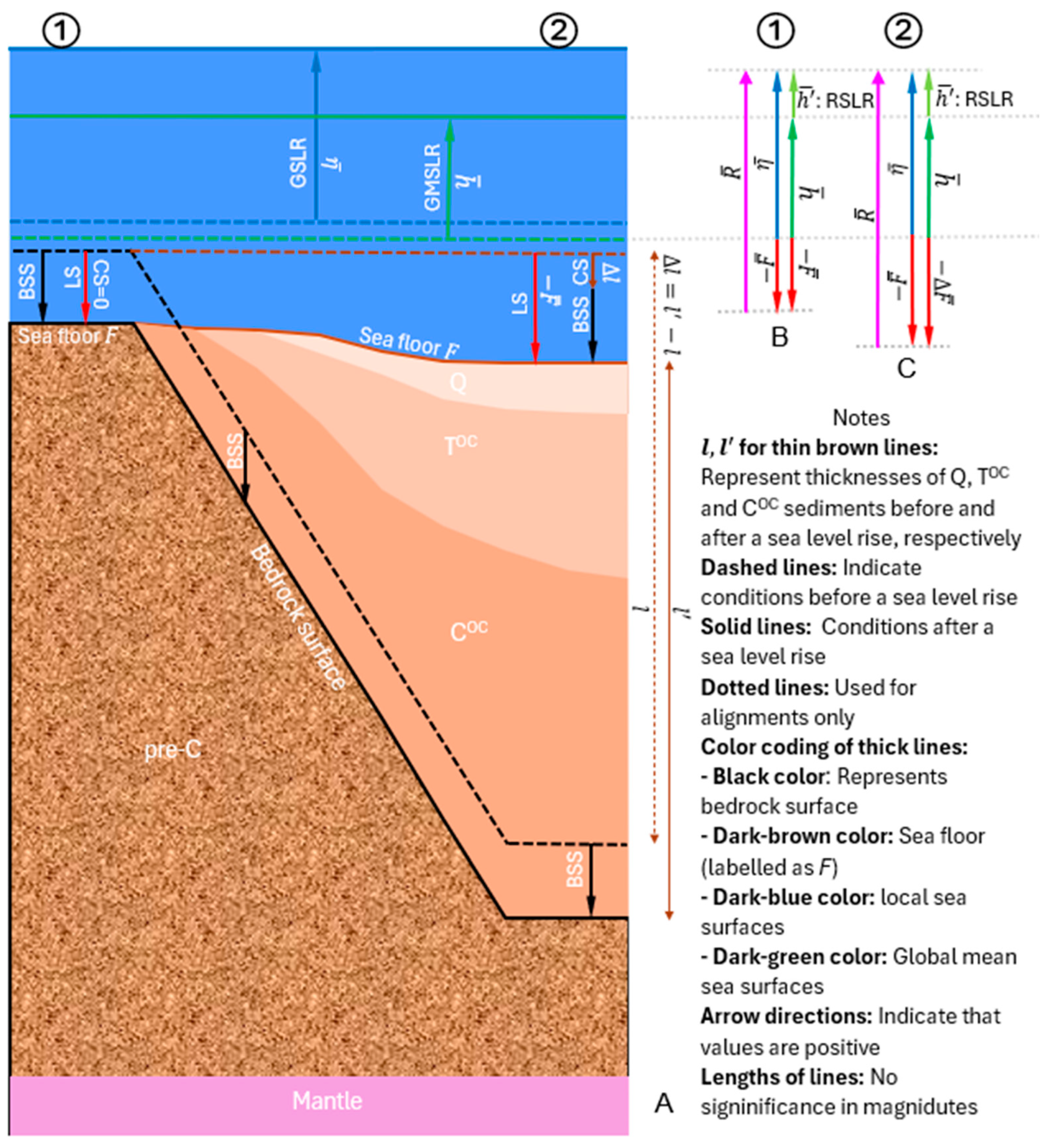
Equation (11) is employed in Figure 4 to conceptually illustrate relationships of RSLC at two typical locations, labeled ① and ②, with local LS, RSLR, and GMSLR in Chesapeake Bay. Notably, there is no compaction subsidence (CS) of sedimentary materials at Location ①, whereas such subsidence is present at Location ②.
Figure 4. Conceptual relationships of GSLC (geocentric sea-level change) with RSLR (regional sea-level rise), GMSLR (global mean sea-level rise) and local LS (land subsidence) in Chesapeake Bay. (A) A profile along the coast in a region with tide gauge locations ①: bedrock (pre-C) surface as sea floor and ②: compressible Q, T, and C sediments’ surface as sea floor. (B) Relationships between trend quantities at Location ①. (C) Relationships between trend quantities at Location ②. h ¯ in B and C denotes the regional sea-level rise (RSLR). Shades in the navy color represent changed seawater bodies while the shade in the light blue color represents the unchanged seawater body.
RSLC trend equation: We adopt a user-focused conceptual framework similar to Parris et al. [] and utilized by Sweet et al. [,]. According to this framework, sea level rose linearly from 1900 to 1992 and has risen or is projected to rise quadratically from 1992 to 2100. This acceleration since 1992 coincides with global sea-level acceleration overserved via altimetry since 1993 [].
Using Maclaurin series, we define η ¯ t = η ¯ 0 + i = 1 α i η t i and F ¯ t = F ¯ 0 + i = 1 α i F t i , where η ¯ 0 , F ¯ 0 , α i η , and α i F are constants when its derivative in any order exists. Based on the definition of RSLC, we have R ¯ t = η ¯ F ¯ = η ¯ 0 F ¯ 0 + i = 1 α i η α i F t i = R ¯ 0 + i = 1 α i η α i F t i , where η ¯ 0 , F ¯ 0 , and R ¯ 0 are intercept constants. The rate of RSLC trend is R ¯ ˙ t = α 1 η α 1 F + i = 2 α i η α i F t i 1 = R ¯ c + R ¯ ˙ n , where R ¯ c = α 1 η α 1 F which is called the linear constat of RSLC trend and R ¯ ˙ n = i = 2 α i η α i F t i 1 which can be called the non-linear rate of RSLC trend as in []. If η ¯ is quadratic after t 0 and F ¯ linear, R ¯ ˙ n =   α 2 η t , we have
R ¯ t = R ¯ 0 + R ¯ c t ,   t t 0
R ¯ t = R ¯ 0 + R ¯ c t + 0.5 α 2 η t t 0 2 ,   t t 0
where α 2 η denotes the acceleration of the RSLC trend. Equations (12) and (13) represent a complete RSLC trend formulation with two phases, following Parris et al.’s framework, by defining 1900 t 2100 and t 0 = 1992 . The two equations can be applied to any long-term tide gauges for identifying RSL R ¯ 0 in 1900, RSLC rate R ¯ c , and RSLR acceleration α 2 η through inverse simulation. However, a less than 0.01 mm/year stability of linear RSLC trend rate R ¯ c requires a data timescale of at least 122 years when Equations (12) and (13) are independently applied to a long-term tide gauge (see Section 4.1). Only the tide gauge of Baltimore, served 122 years since 1902 in the study area, meets this requirement.
Parris et al.’s GMSLR trend equation: Parris et al. (2012) [] suggested trend of GMSLR h ¯ as
h ¯ t = h ¯ 0 + α 1 h t ,   t t 0
h ¯ t = h ¯ 0 + α 1 h t + 0.5 α 2 h t t 0 2 ,   t t 0
where h ¯ 0 , α 1 h , and α 2 h are constants, representing GMSL in 1900, linear GMSLR rate, and GMSLR acceleration since 1992, respectively, 1990 t 2100 , and t 0 = 1992 . Sweet et al. (2017, 2022) [,] utilized Equation (12). Dangendorf et al. (2017) [] found α 1 h be 1.1 ± 0.3 mm/year between 1902 and 1990 [] from global tide gauge data. Nerem et al. found α 2 h to be 0.084 ± 0.025 mm/year2 [] from altimetry global mean sea-level data with α 1 h of 1.70 mm/year between 1900 and 2009 and 1955 and 2000 [,], respectively. Part 2 will show that a α 2 h value of 0.120 ± 0.025 mm/year2 is derived from altimetry global mean sea-level data by using the α 1 h value of 1.1 ± 0.3 mm/year. It futher suggests using 1.1 ± 0.3 mm/year as a linear GMSLR trend rate and 0.120 ± 0.025 mm/year2 as GMSLR acceleration in Parris et al.’s framework.
RSLR trend equation based on Parris et al.’s framework: The trend of h can be written as
h ¯ t = h ¯ 0 + α 1 h t ,   t t 0
h ¯ t = h ¯ 0 + α 1 h t + 0.5 α 2 h t t 0 2 ,   t t 0
where h ¯ 0 , α 1 h , and α 2 h are constants, representing regional sea level in 1900, linear RSLR rate, and RSLR acceleration since 1992, respectively, 1990 t 2100 , and t 0 = 1992 . The linear RSLR rate α 1 h can be found using Equation (14):
α 1 h = R ¯ c α 1 h + α 1 F
If a stable RSLC rate R ¯ c can be found from a long-term tide gauge such as tide gauge Baltimore through inverse simulation by using Equations (12) and (13), the LS rate α 1 F can be determined from GPS measurement or Interferometric Synthetic Aperture Radar (InSAR) data, and the GMSLR rate α 1 h of 1.1 ± 0.3 mm/year [] is employed.
RSLC trend equation in terms of RSLR, GMSLR, and local LS based on Parris et al.’s framework: Associating Equations (12) and (13) with a combination of Equations (14) and (15) as well as (16) and (17) yields
R ¯ t = h ¯ 0 + h ¯ 0 F ¯ 0 + α 1 h + α 1 h α 1 F t ,   1900 t 1992
R ¯ t = h ¯ 0 + h ¯ 0 F ¯ 0 + α 1 h + α 1 h α 1 F t + 0.5 α 2 h + α 2 h t t 0 2 , 1992 t 2100
where h ¯ 0 + h ¯ 0 F ¯ 0 = η ¯ 0 F ¯ 0 = R ¯ 0 in Equations (12) and (13), i.e., intercept of RSLC trend; α 1 h + α 1 h α 1 F = α 1 η α 1 F = R ¯ c in Equations (12) and (13), i.e., linear constant rate of RSLC trend; and α 2 h + α 2 h = α 2 η , i.e., acceleration of RSLC trend in Equation (13). α 1 h , a linear component of RSLR, and α 2 h , the quadratic acceleration of RSLR, can be estimated from R ¯ c and α 2 η values derived from local tide gauge data by using Equations (12) and (13), α 1 h values such as 1.1 ± 0.3 mm/year [], and α 2 h values from global altimetric sea level data such as 0.084 ± 0.025 mm/year2 []. An average α 2 h value of 0.0991 mm/year2 is found by using the α 1 h value of 1.1 ± 0.3 mm/year in Part 2 of this paper. The linear part of Equations (12) and (13) can be changed to piecewise forms if needed.
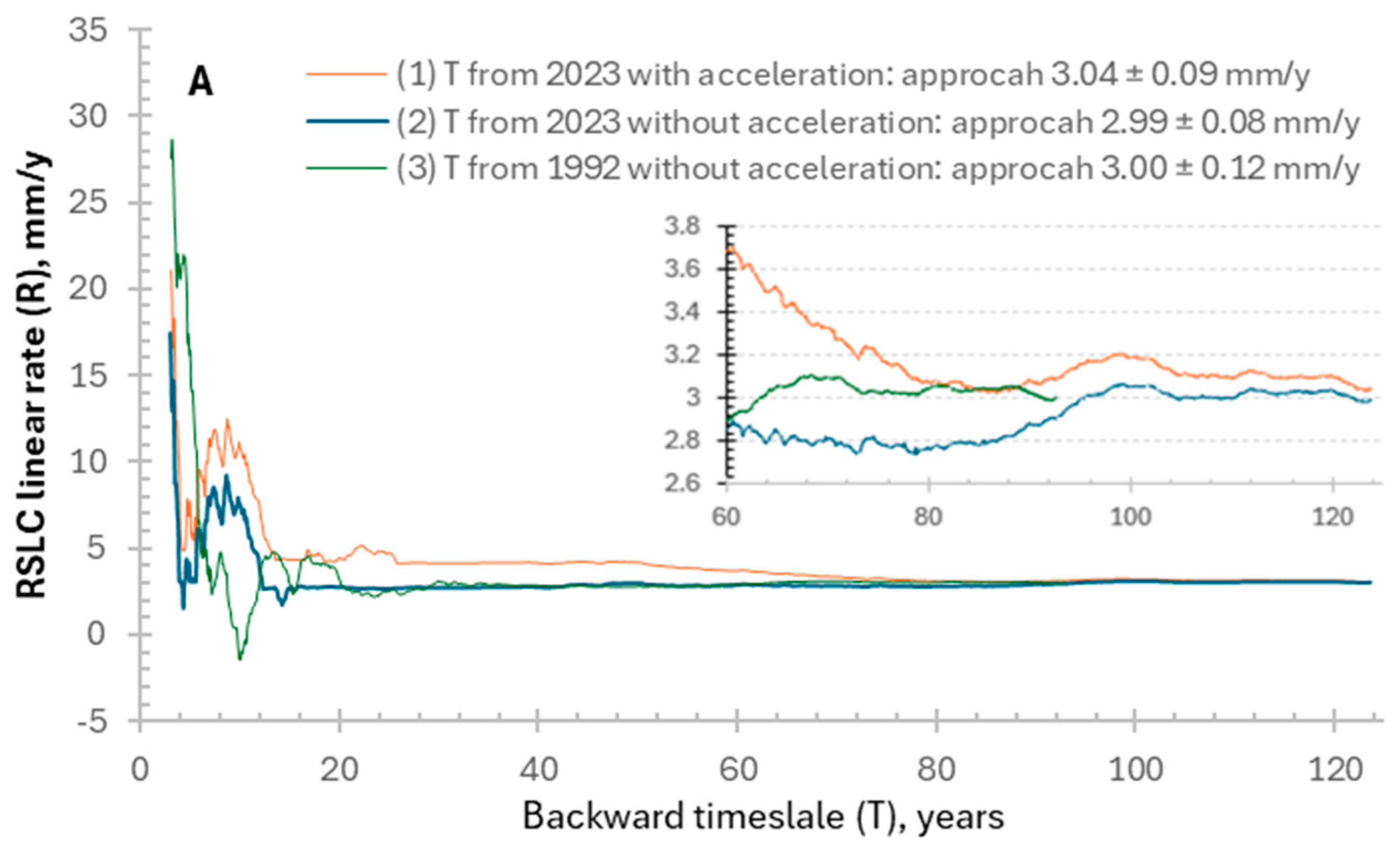
The variation in the RSLC linear constant R ¯ c with data timescales (hereafter T), ranging from 3.0 to 123.7 years, is analyzed using NOAA tide gauge data from the New York Battery tide gauge, which has the longest data timescale in the U.S. at 168 years.
In summary, a best estimate of the linear GLMSL trend since 1990 from global tide gauge data can be used to determine its acceleration since 1992 through quadratic fitting of satellite altimetry global sea-level data. These two quadratic parameters can then be incorporated into RSLC trend simulations from a single long-term tide gauge record and used for RSLC trend projections.

4. Methodology for Estimating LS Using Short-Term Tide Gauge Data

4.1. Reference Tide Station in the Study Area—Tide Gauge Baltimore

Finding a constant LS rate ( F ¯ ˙ , i.e., α 1 F in Equations (19) and (20)) from tide gauge data depends on the stability of the RSLC linear constant R ¯ c , defined as α 1 h + α 1 h α 1 F in Equation (12). This study assumes that R ¯ c remains stable within 0.01 mm/year since NOAA’s calculated RSLC trends are two decimals in millimeters/year. The LS rate (− α 1 F ) can be assumed to be constant since this tide gauge is seated on Ordovician (?) Manhattan Formation bedrock [] (pre-C). A linear RSLC function R ¯ of time t is employed to find linear RSLC trend rate R ¯ c [i.e., α 1 h + α 1 h α 1 F in Equation (16)]. Figure 5A shows how R ¯ c varies with T under three conditions: (1) raw monthly mean relative sea-level data with sea-level rise acceleration since 1992, for T values ranging from 3.0 to 123.7 years, measured backward from the start year 2023; (2) monthly mean relative sea-level data without sea-level rise acceleration since 1992, for T values from 3.0 to 123.7 years, measured backward from 2023; and (3) monthly mean relative sea-level data without sea-level rise acceleration since 1992, for T values from 3.0 to 92.6 years, measured backward from 1992. The analysis reveals that (a) R ¯ c stability improves as T increases; (b) the best estimate of a stable R ¯ c is 2.99 ± 0.08 mm/year for dataset (2) with T  122 years; and (c) removing the nonlinear trend (i.e., accelerated sea-level rise component) enhances the stability for data timescales shorter than about 72 years (short-term tide gauges), further supporting the existence of RSL acceleration since 1992 in Parris et al.’s framework. This implies that achieving R ¯ c stability within 0.01 mm/year requires a tide gauge data period spanning at least 122 years (from 2023 back to 1902). Additionally, using tide gauge data periods shorter than 60 years may result in deviations in the RSLC linear trend, ranging from −1.43 mm/year for T = 9.4 years to approximately 28.64 mm/year for T = 3.1 years, compared to the long-term stability value of 2.99 mm/year. For tide gauge data spanning 46 and 100 years, deviations in the RSLC linear trend range from 2.74 mm/year to approximately 3.06 mm/year, with departures of −0.25 to 0.07 mm/year from the long-term stability of 2.99 mm/year (see Figure 5B). Among Chesapeake Bay tide gauges, only the Baltimore tide gauge has operated more than 122 years since 1902, while the other 14 tide gauges in the region range from 46 years (Wachapreague, VA, USA) to 100 years (Washington, DC, USA). This means the 14 short-term tide gauges cannot be directly employed to determine a constant LS rate F ¯ ˙ (i.e., α 1 F ) in Equation (16) with precision better than 0.01 mm/year through simple linear or quadratic regression of RSLC over time. To overcome this limitation, we propose a new methodology to derive constant LS rates from the 14 short-term tide gauges by linking to the long-term Baltimore tide gauge. In this methodology, the Baltimore tide gauge serves as the Reference Tide Station in the Chesapeake Bay area for estimating the constant LS rate at the other 14 tide gauge locations. This is justified because it meets the R ¯ c stability requirement of a 122-year data period and has a known LS rate of 1.86 mm/year [] (see Figure 1).
Figure 5. Variation in linear RSLR rate (R) with data timescale (T) at the New York tide gauge (NOAA ID: 8518750). (A) R changes with T from a start year (such as 2023) backward to an end year. The inset graph provides a zoomed-in illustration of T from 60 to 120 years. (B) Absolute error of R relative to a best R estimate of 2.99 mm/year with the end year of a T in A.

4.2. Equation for Estimating LS at a Short-Term Tide Gauge

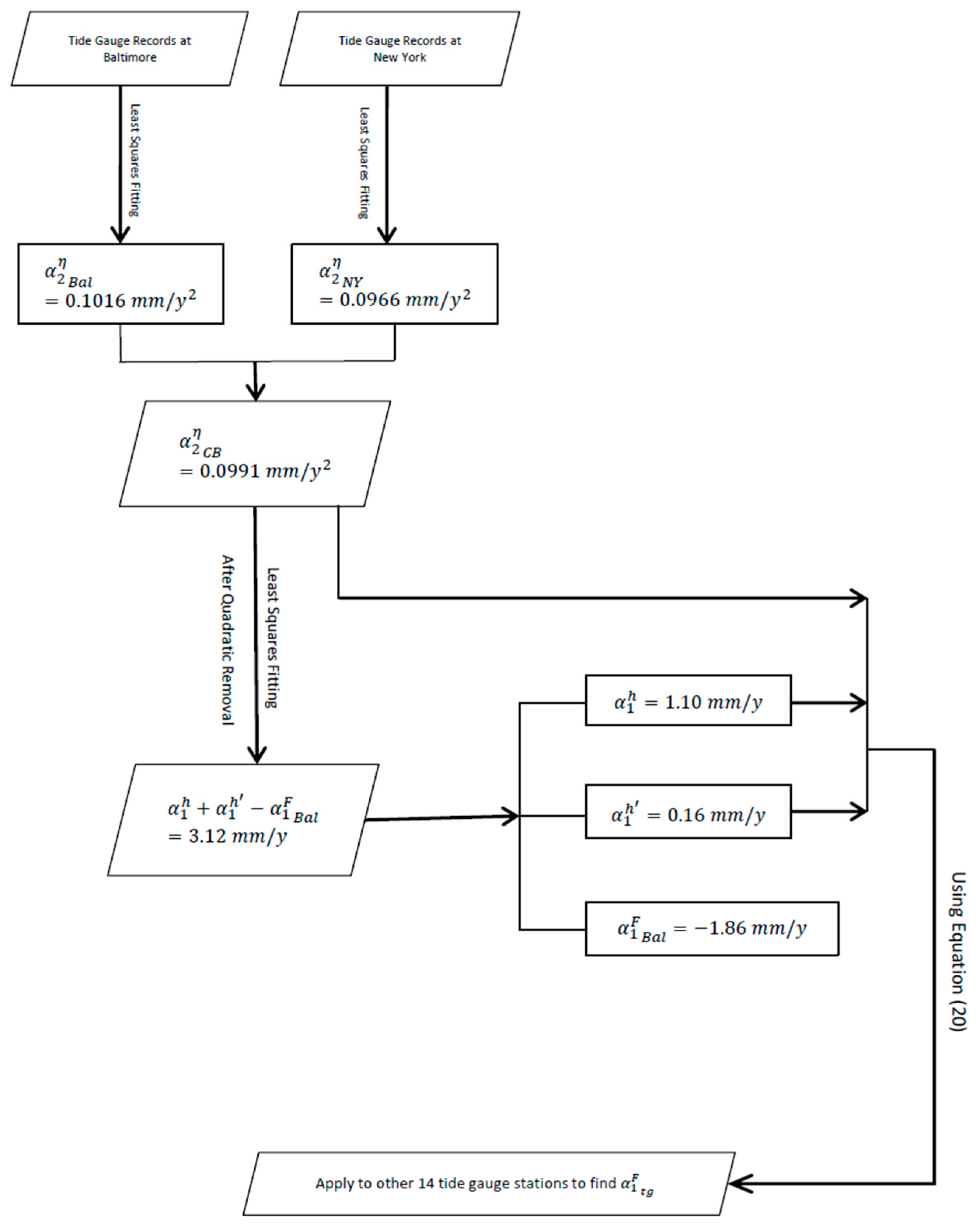
Figure 6 shows that GSLC acceleration of 0.1016 mm/year2 simulated from each tide gauge’s monthly mean sea-level time series can be reformed by removing climate-change-driven accelerated sea-level rise since 1992 [] using the acceleration of 0.0991 mm/year2 established in Figure 6. From the reformed sea-level data, linear RSLC trend equations can be written as Equation (21) for tide gauge Baltimore and (22) for any of the other 14 tide gauges with a data timescale T between 46 and 100 years in the study area according to Equation (19):
R ¯ t B a l = R ¯ 0 B a l + β B a l α 1 h + α 1 h α 1 F B a l t
R ¯ t t g = R ¯ 0 t g + β t g α 1 h + α 1 h α 1 F t g t
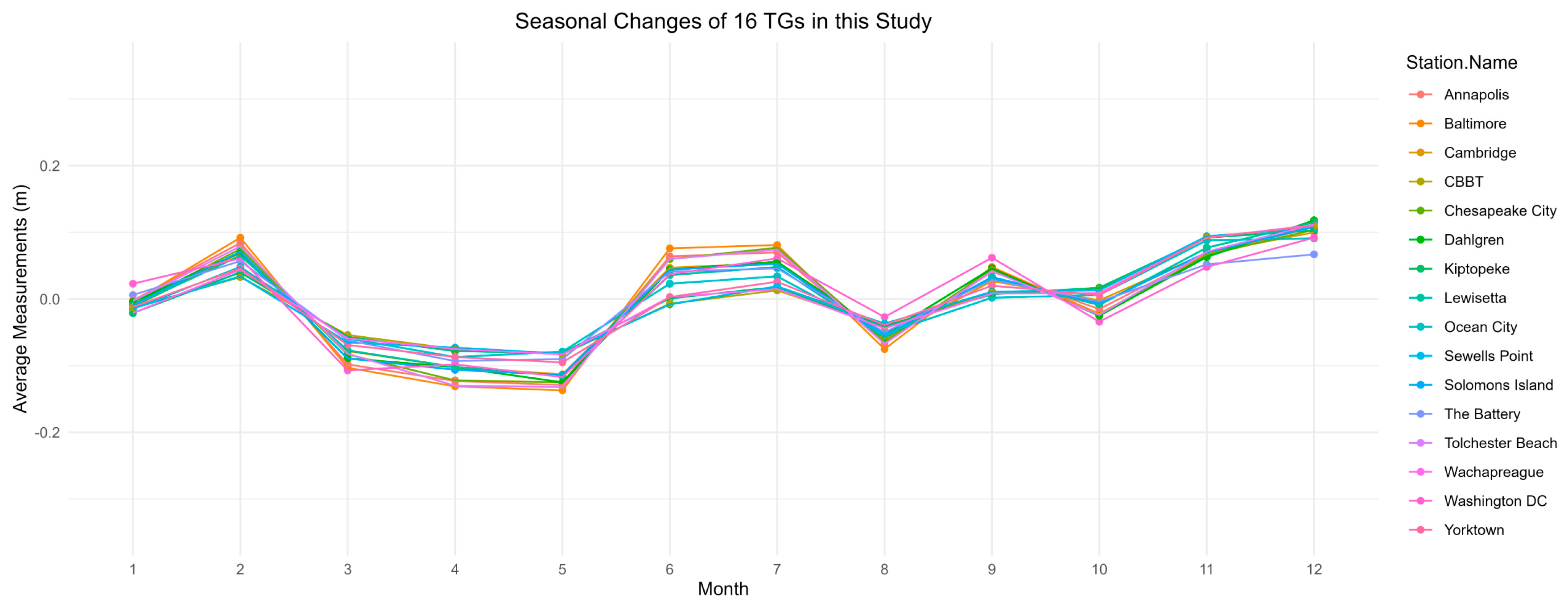
where t is time in years; β B a l and β t g are constant to make the stable linear RSLC trend rates α 1 h + α 1 h α 1 F B a l = R ¯ c B a l and α 1 h + α 1 h α 1 F t g = R ¯ c t g vary to β B a l α 1 h + α 1 h α 1 F B a l and β t g α 1 h + α 1 h α 1 F t g , respectively, due to a short data timescale T. Figure 5B shows the β value of the tide gauge Battery varies from 0.916 to 1.025 for T between 46 and 100 years. R ¯ t t g can be derived as a linear function of R ¯ t B a l as Equation (23):
R ¯ t t g = β t g β B a l α 1 h + α 1 h α 1 F t g α 1 h + α 1 h α 1 F B a l R ¯ t B a l   + R ¯ 0
where R ¯ 0 is a constant or an intercept. Equation (23) becomes Equation (24) if β B a l β t g , which requires that variations in monthly mean sea levels are similar at all tide gauges in the Chesapeake Bay area.
R ¯ t t g = k t g B a l R ¯ t B a l + R ¯ 0
where k t g B a l = α 1 h + α 1 h α 1 F t g / α 1 h + α 1 h α 1 F B a l . β B a l β t g may be supported by the similarity of monthly mean sea-level variations at the 15 tide gauges in the Chesapeake Bay area and the tide gauge Battery in New York shown in Figure 7. Supplementary Figure S1(A1–O1) shows similarity of 11-month moving average sea-level variations between tide gauge Baltimore and each of other 14 tide gauges and tide gauge Battery in New York in different time windows. Since we find α 1 h +   α 1 h = α 1 η = 1.26   m m / y e a r in the Chesapeake Bay region and the LS rate α 1 F B a l at the Baltimore tide gauge location is 1.86 mm/year [] (see Figure 1), then the LS rate α 1 F t g at a short-term tide gauge can be solved by using Equation (24) if k t g B a l is known:
α 1 F t g = ( α 1 h + α 1 h α 1 F B a l )   k t g B a l ( α 1 h α 1 h ) = ( α 1 η α 1 F B a l )   k t g B a l α 1 η
Figure 6. The flowchart illustrates the processes for determining LS rates ( α 1 F t g ) at 14 short-term tide gauge sites in the Chesapeake Bay region.
Figure 7. Seasonal changes in average water level measurements at the 16 tide gauge stations (15 in Chesapeake Bay and one at “The Battery” in New York), based on data released on the NOAA website. (Example for the tide gauge in Baltimore.)
Equation (25) shows the relationship of a long-term LS trend rate ( α 1 F t g ) at each of the 14 short-term tide gauges with linear GMSLR rate α 1 h , RSLR rate α 1 h , and local LS rate ( α 1 F B a l ) at the Baltimore tide gauge location through a linear regression coefficient k t g B a l of RSLC between the short-term tide gauge and reference tide station Baltimore. In the Chesapeake Bay area, Equation (25) becomes
α 1 F t g = ( 1.26 α 1 F B a l )   k t g B a l + 1.26
Supplementary Figure S1(A2–O2) shows k t g B a l values for all the 14 short-term tide gauges with the R-squared values of 0.91 to 0.99 excluding Baltimore. LS rates (i.e., α 1 F t g ) at the 14 tide gauge locations can be found from the k t g B a l values using Equation (26).

4.3. Evaluation of Uncertainty and LS Rate Range Under 95% Confidence Interval

4.3.1. Pearson Correlation Coefficient and Its Confidence Interval

In our methodology, linear correlations can be established as in Supplementary Figure S1(A2–O2) between each short-term tide gauge and reference tide station Baltimore, as well as between tide gauges Baltimore and New York, under short data timescale windows. To minimize the influence of high-frequency and seasonal variability, 11-month moving averages were applied to the relative sea level time series prior to calculating correlations. The original trends were preserved because the objective was to assess shared variability rather than to remove long-term signals. Time windows were defined based on overlapping observation periods between the Baltimore reference station and each short-term tide gauge to maximize data comparability. As the stations are located in the same estuarine system and subject to similar large-scale forcing, high correlation coefficients are expected and reflect regional coherence rather than purely site-specific dynamics. The Pearson correlation coefficient is the primary measure of the linear relationship, and its corresponding 95% confidence interval can be calculated by considering the sample size and the standard error of the Fisher-transformed correlation coefficient. The list of statistics is displayed in Table 1.
Table 1. The evaluation of uncertainty at each tide gauge station.
Take the Annapolis tide gauge as an example. There are 1083 samples (see D1 values in column 5) on relative sea levels from the overlapping period between the Annapolis and Baltimore tide gauge stations. The statistical results suggest that there is 95% confidence that the Pearson correlation coefficient lies within the range of 0.993 to 0.995 (larger values in C6 and C7 columns at TG Annapolis). Similarly, there is 95% confidence that the Pearson correlation coefficient between the tide gauges of New York and Baltimore, within the same time window, lies within the range of 0.990 to 0.992 (C6 and C7 values at TG Baltimore).

4.3.2. Max and Min LS Rate Under the 95% Confidence Interval

Equation (25) or (26) suggest that the LS rate at any short-term tide gauge station can be calculated using the inferred k N Y B a l and k t g B a l parameters, derived from the overlapping time window comparisons as described above. This approach allows the linear subsidence component to be inferred from stations with shorter records. Across the 15 stations, the inferred LS rates fall within the range of 1.86 to 2.88 mm/year, reflecting both shared regional forcing and local variability. Considering the upper and lower estimates under the 95% confidence interval, there are upper and lower ranges for the inferred k N Y B a l and k t g B a l parameters. As a result, there exists a maximum and a minimum value for the LS rate ( α 1 F t g ) . The LS rate range at the 15 tide gauge stations under the 95% confidence interval is presented in Table 1 of Part 2.

5. Methods for Analyzing Components of LS

Categorization: We classify the LS ( F ¯ ) trend in Figure 4 into two major categories: bedrock-surface subsidence (BSS) from geological material bedrocks (pre-C) and the mantle below the bedrock surface in response to global glacial isostatic adjustment (GIA) processes (see details for BBS in Appendix B), and compaction subsidence (CS) of compressible sediments (COC, TOC, and Q) between the sea floor and bedrock surface in response to local non-GIA processes [] as shown in Table 2. Global GIA processes may include GIA itself, tectonics, earthquake, and volcano activities, etc. [,,,,,], while local non-GIA processes may include sediments’ creep, groundwater pumping from aquifers, weathering, land sliding, erosion, sedimentation, construction operation, biomass growth, among others, in human time. Sediments between the sea floor and bedrock surface in the Chesapeake Bay region include very thin (~50 m thick) Quaternary sediments (Q), Quaternary surficial aquifer (QW) (Figure 8), minor Tertiary aquifer-systems (TOC), and major Cretaceous aquifer systems (COC) (Figure 8). The thickness of the sediments may be up to 2230 m (Figure 8). There may exist the following potential CS in the sediments in the Chesapeake Bay area: (1) primary consolidation subsidence (PCS) of the minor Tertiary aquifer systems (TOC) and the major Cretaceous aquifer systems (COC) (Figure 8) due to groundwater pumping (see details for PCS in Appendix C); (2) the secondary consolidation subsidence (SCS) of normally consolidated Quaternary sediments (Q) and over-consolidated aquifer systems (TOC and COC) resulted from natural overburden pressure [,] (see details for SCS in Appendix D); (3) construction-induced subsidence (CIS) attributable to the anthropogenic processes related to construction activities, such as tunnels and subways in the urbanization process [,] (see details for CIS in Appendix E); and (4) the negative subsidence (NS)—vertical expansion of surficial aquifers (QW) from its parent rock-like TOC and COC sediments due to current weathering [] or sedimentation and biomass growth of soils (Q) in wetland [] (see details for NS in Appendix F).
Table 2. Geological type and symbol of tide gauges in the study area [modified from [].
Figure 8. Typical cross-section of the Atlantic Coastal Plain aquifer system in the Chesapeake Bay region (modified from []). Surficial aquifer (QW) is weathered product of Tertiary aquifer system (see Supplementary Figure S8). Aquifer systems shaded in gray in the cross-section are in Cretaceous (COC) and Tertiary (TOC) sediments.
LS estimating: Only LS of 1.86 mm/year at reference tide station Baltimore in Figure 1 is estimated from LS on the US east coast detected from InSAR image data by Ohenhen et al. (2023) []. LS ranges of 1.92 to 3.12 mm/year at the other 14 tide gauge locations are found by using Equation (19) from linear correlation coefficient k t g B a l values in Supplementary Figure S1(B2–O2), which is shown in Part 2 in detail.
BBS contour mapping: LS = CS + BSS generally. LS = BSS if bedrock surface is equal to the sea floor, i.e., CS = 0 (see CS at location ① in Figure 4). Only tide gauge Washington, D.C. is seated on the pre-C bedrock surface without CS. CS is negligible at three tide gauge locations, Baltimore and Ocean City in Maryland, and Kiptopeke in Virginia, through analysis in Part 2 using comprehensive methods in Appendix B, Appendix C, Appendix D, Appendix E and Appendix F using groundwater level data in eight wells as shown in Supplementary Figure S2. LS values found by using methods in Section 3 and Section 4 can be determined to be their BBS values at the four tide gauge locations, respectively. The four BBS values allow us to map the first BSS contours in the range of 1.48 to 2.42 mm/year in the Chesapeake Bay region. Results are shown in Part 2 in detail.
CS estimating: CS in the range of 0 to 0.75 mm/year at the 15 tide gauge locations can be estimated from the determined LS above at each tide gauge location by removing BBS interpolated from the above BBS contours. Results are shown in Part 2 in detail.
CS type determination: Methods in Appendix C, Appendix D, Appendix E and Appendix F are employed to analyze PCS, SCS, CIS, and NS at each tide gauge location based on geological, geohydrological, and soil mechanical information. SCS in over-consolidated Tertiary and Cretaceous sediments (TOC and COC in Figure 8 and Table 2) can be ignored since the sediment strata was uplifted during Quaternary. SCS of less than 0.01 mm/year in Quaternary sediments can be ignored as well since the Quaternary sediment thickness is thin (see Figure 8). PCS of up to 0.75 mm/year is present at nine tide gauge locations, including Cambridge, Solomons Island, Annapolis and Tolchester Beach in Maryland, and Sewells Point, Yorktown, Lewisetta, Dahlgren, and Wachapreague in Virginia. CIS of 0.52 mm/y during 1960–1990 is estimated at CBBT (Chesapeake Bay Bridge Tunnel) in Virginia. Results are shown in Part 2 in detail.
Figure 9 summarizes the above workflow for deciphering LS into BBS and CS and further dividing CS into PCS and CIS.
Figure 9. A flowchart for deciphering LS into BBS and CS and further dividing CS into PCS and CIS.

6. Projection Equation of RSLC in Terms of GMSLR, RSLR, and LS

Equation (20) can be built to project RSLC by 2100 for each of the 15 tide gauges in the Chesapeake Bay region with identified values for two GMSLR parameters α 1 h and α 2 η , two RSLR parameters α 1 h and α 2 h , LS ( α 1 F ) , and intercept R ¯ 0 ( = h ¯ 0 + h ¯ 0 F ¯ 0 ). Contributions from GMSLR, RSLC, and LS can be computed over time. Projection results are shown in Part 2.

7. Conclusions

This study presents a novel, integrated methodology to decipher relative sea-level change (RSLC) in Chesapeake Bay by disentangling the contributions of global mean sea-level rise (GMSLR), regional sea-level rise (RSLR), and local land subsidence (LS). By combining long-term tide gauge records, satellite altimetry, and InSAR observations, we derive trend equations spanning from 1900 to 2100 and establish a robust framework to estimate both linear and nonlinear RSLC trends using trend equations and Maclaurin series expansions.
A key contribution of this work is the development of an innovative approach to estimate LS at short-term tide gauges by referencing long-term data from the Baltimore station, which meets the minimum 122-year threshold required for stable RSLC trend estimation. This technique enables more accurate LS assessments across Chesapeake Bay, even in locations lacking long-term data. Additionally, we classify LS into bedrock-surface subsidence (BSS) and compaction subsidence (CS), further subdividing CS into four types—primary consolidation, secondary consolidation, construction-induced, and negative subsidence—based on sediment types and geologic conditions. These classifications provide an important basis for identifying spatial heterogeneity in land motion and understanding underlying mechanisms.
The methodology proposed here not only advances sea-level trend analysis in sediment-rich and tectonically quiet estuarine environments like the Chesapeake Bay but also sets a foundation for applying similar techniques in other vulnerable coastal regions. By integrating geophysical, oceanographic, and geotechnical insights, this work enhances the precision of RSLC assessments, supporting long-term resilience planning, infrastructure design, and risk mitigation strategies in the face of accelerating sea-level rise.
In Part 2 of this two-part study, we will apply the methodology developed here to produce spatially distributed projections of RSLC, quantify uncertainties, and analyze site-specific risk across Chesapeake Bay. Together, both parts aim to provide a comprehensive framework for addressing the scientific and societal challenges posed by coastal sea-level changes.

Supplementary Materials

The following supporting information can be downloaded at: https://www.mdpi.com/article/10.3390/w17213167/s1. Figure S1. The correlation of reformed 11-month moving average relative sea levels between tide gauge Baltimore and each of 14 short-term tide gauges. Figure S2. The groundwater level time series of 8 wells near TGs Baltimore, Washington D.C., TG Ocean City and Kiptopeke, and graphs acquired from USGS National Water Information System. Figure S3. Two examples of compaction subsidence (CS) in the United States. Figure S4. Subsidence due to secondary consolidation (creep) subsidence (SCS) and historical changes in effective stress presented with a conceptual isotache model. Figure S5. Time series of cumulative line-of-sight (LOS) displacement for the selected persistent scatterer (PS) points along tunnel A-A’ in Dangjin, Korea. Figure S6. Conceptual model of negative subsidence (NS) from land growth caused by vertical expansion of bedrock to soil+saprolite+fractured-rock due to weathering in Quaternary. Figure S7. Land loss due to erosion and land accretion due to sedimentation and biomass growth between subtidal, intertidal, and terrestrial ecosystems in coastal marshland. Figure S8. A photo of the surficial sediment. Surficial aquifer (QW) of weathered subcrop Chesapeake Group/Choptank Formation sandstone and siltstone (Miocene of Tertiary) at Calvert Cliffs.

Author Contributions

Y.L. and X.Z. designed research; Y.L. and X.Z. performed research; X.Z. and Y.L. analyzed data; and Y.L. and X.Z. wrote the paper. All authors have read and agreed to the published version of the manuscript.

Funding

This research is primarily funded by the National Science Foundation (NSF) through Grant #2101056, titled “Identification of absolute sea-level rise and land subsidence from long-term TG records along coasts of the Gulf of Mexico and the Chesapeake Bay.” Additionally, there is a secondary source of support from the Department of Energy (DOE) Grant DE-SC0023276 under the project “Baltimore Social-Environmental Collaborative.” The opinions, results, and conclusions or recommendations presented in this work are solely those of the author(s) and do not necessarily represent the views of the NSF and the DOE.

Data Availability Statement

The original contributions presented in this study are included in the article and Supplementary Materials. Further inquiries can be directed to the corresponding author.

Acknowledgments

The authors also appreciate the insightful and constructive comments provided by Torbjörn Törnqvist to the previous version and three anonymous reviewers to the current version, which led to significant improvements.

Conflicts of Interest

The authors declare no conflicts of interest.

Abbreviations and Notation

BSSBedrock-surface subsidence
CBChesapeake Bay
CBBTChesapeake Bay Bridge Tunnel
CISConstruction-induced subsidence
CSCompaction subsidence
GIAGlacial isostatic adjustment
GMSLRGlobal mean sea-level rise
GRDGravitational, rotational, and deformational
GSLCGeocentric sea-level change
HRSDHampton Roads Sanitation District
LSLand subsidence
MSLMean sea level
NSNegative subsidence
PCSPrimary consolidation subsidence
RSLCRelative sea-level change
RSLRRegional sea-level rise
SCSSecondary consolidation subsidence
TGTide gauge
VLMVertical land motion
B Inverse barometer (IB)
Δ B Change of IB
CNormally consolidated Cretaceous sediment layer
COCOver consolidated Cretaceous sediment layer
Δ E The impact effect of global GRD to regional sea level such as in Chesapeake Bay region, i.e., Δ Γ Δ F + Δ E at any oceanic location
F Sea floor height
Δ F Vertical land motion (VLM)
Δ F The deviation of the change in the sea floor from its respective global (ocean) mean
F ¯ Trend of sea floor height
F ¯ 0 Trend of sea floor height in 1900
F ¯ ˙ Trend rate of sea floor height
G Geoid
Δ G Change in geoid height
Δ G The deviation of the change in the geoid from its respective global (ocean) mean
h Global mean sea-level rise (GMSLR)
h RSLR, i.e., Δ ζ + E B in Equation (5)
h ¯ GMSLR trend
h ¯ RSLR trend
h ¯ 0 GMSLR trend in 1900
h b Barystatic SLR
h b Global mean thermosteric SLR
H The thickness of ocean
Δ H H change
k t g B a l Linear correlation coefficient of 11-month relative sea levels between a short-term Tide gauge and reference tide gauge Baltimore
l The thickness of compressible sediments before a sea-level rise
l The thickness of compressible sediments after a sea-level rise
Δ l Compaction subsidence (CS)
QQuaternary sediment layer
QhHolocene sediments
QhPleistocene sediments
QwWeathering product of Tertiary and Cretaceous strata during Quaternary
Q h w Weathering product of Tertiary and Cretaceous strata during Holocene
Q p w Weathering product of Tertiary and Cretaceous strata during Pleistocene
R2Squared regression coefficient
Δ R Relative sea-level change (RSLC)
Δ R m Manometric SLC
Δ R s Halosteric SLC
Δ R θ Thermosteric SLC
Δ R ρ Steric SLC
R ¯ RSLC in trend
R ¯ 0 RSLC in trend in 1900
R ¯ c Linear RSLC rate (constant) in trend
R ¯ ˙ n The nonlinear rate of RSLC trend
t Time in years between 1900 and 2100
t 0 1992
TNormally consolidated Tertiary sediment layer
TOCOver-consolidated Tertiary sediment layer
Δ Z Sterodynamic SLC
α i F Constant i of variable time t to the i th power for a Maclaurin series of F ¯
α i η Constant i of variable time t to the i th power for a Maclaurin series of η ¯
α 2 η B a l Acceleration of RSLR trend η ¯ from reference tide station Baltimore since 1992
α 2 η N Y Acceleration of RSLR trend η ¯ from tide gauge Battery in New York since 1992
α 2 η C B Average acceleration RSLR trend η ¯ for Chesapeake Bay
α 1 h Linear constant rate of GMSLR trend h ¯
α 2 h Acceleration of GMSLR trend h ¯ since 1992
α 1 F Linear constant rate of VLM trend F ¯
α 1 F Linear constant rate of LS trend ( F ¯ )
α 1 F B a l α 1 F at reference tide station Baltimore
α 1 F t g α 1 F at any short-term tide gauge
α 1 h Linear constant rate of RSLR trend h ¯
α 2 h Acceleration of RSLR trend h ¯ since 1992
α 2 h B a l Acceleration of RSLR trend h ¯ since 1992 derived from tide gauge data at Baltimore
β Ratio of short-term linear RSLC trend rate R ¯ c to its long-term stable rate
Δ ζ Ocean dynamic SLC
η Geocentric sea level
Δ η Geocentric SLC
η ¯ Geocentric sea level in trend
η ¯ 0 Geocentric sea level in trend in 1900
Δ Γ GRD: changes in Earth’s gravity, Earth’s rotation (and, hence, centrifugal acceleration) and viscoelastic solid-Earth deformation

Appendix A. GRD—Changes in Earth’s Gravity, Earth’s Rotation (and Hence Centrifugal Acceleration) and Viscoelastic Solid-Earth Deformation [] (Gregory et al., 2019)

These three effects are all caused by changes in the geographical distribution of ocean and solid mass over Earth. They are often considered together because they occur simultaneously and may interact. Changes in gravitation and rotation alter the geopotential field and, hence, the geoid G , while deformation of the solid Earth changes the sea floor topography F through VLM or LS. By altering G and F, GRD induces RSLC (e.g., [,]), which redistributes but does not change the global ocean volume and thus causes no GMSLR. GRD-induced RSLC Δ Γ is defined as
Δ Γ = Δ G Δ F
where Δ G and Δ F are the deviations of the changes in the geoid and in the sea floor from their respective global (ocean) means. By construction, the global (ocean) means of G and F are each zero; hence, the global (ocean) mean of Δ Γ is zero. Whatever the cause, redistribution of the ocean mass itself has GRD effects, and the ocean thereby affects its own mass distribution and mean sea level (MSL). Thus, MSL, the geoid and the sea floor must all be related in a self-consistent solution, which in the context of glacial isostatic adjustment (GIA) is expressed by the sea-level equation [].
The ocean GRD effects are called self-attraction and loading (SAL), where “loading” means the weight on the solid Earth. SAL is caused by climatic change in ocean density and circulation [], which do not involve any change in the mass of the ocean. SAL is also a component of GRD which is caused by changes in land ice and in the solid Earth; thus, SAL contributes to the sea-level effects of GIA, contemporary GRD, and mantle dynamic topography as well.
GRD-induced RSLC may be described as the “mass effect”, “mass contribution”, “mass component” or “mass term”, but these labels could equally well refer to manometric sea-level change if local, or barystatic sea-level rise if global, so they can be confusing. Moreover, “GRD” is helpful as a label for a concept which unifies SAL, GIA, contemporary GRD, and mantle dynamic topography.

Appendix B. BSS—Bedrock-Surface Subsidence

The bedrock surface consists of incompressible pre-Cretaceous strata (pre-C). In most of the Chesapeake Bay area, this surface subcrops beneath over-consolidated Cretaceous and Tertiary strata (COC and TOC) and Quaternary sediments (Q) (see Figure 8). In the western and northern parts of the study area, the pre-C strata outcrop locally at land surface. Bedrock surface can coincide with the land or seafloor surface or may lie as deep as up to 2300 m (Figure 8). BSS is measured at a tide gauge’s paired reference GPS station. The GPS antenna is anchored in the pre-C bedrock or over semi-consolidated Tertiary and Cretaceous strata, where primary consolidation subsidence (PCS) and secondary consolidation subsidence (SCS) are negligible []. In the literature, BSS is also called tectonic subsidence (TS) [,,,,,,]. Bedrock creep refers to the gradual deformation of bedrock systems [,]. For this study, we assume the long-term annual rate of bedrock creep as insignificant over the human time scale considered. Global GPS height data from 2567 GPS stations on land are available from the Jet Propulsion Laboratory (JPL) []. Of those, 1961 GPS stations are distributed on the North American Plate, and JPL provides trends (rates) computed for each GPS station. The GPS data are also available from SONEL []. For example, GPS station UMBC is located at the University of Maryland, Baltimore County, Maryland. It is anchored in the pre-Cretaceous Baltimore Gabbro Complex (BGB; Late Precambrian (?) to Early Paleozoic) and lies approximately 12 km west of the Baltimore Inner Harbor tide gauge. We do not use UMBC as the reference GPS station in this study because LS at this location is attributed solely to bedrock-surface subsidence (BSS). SONEL reports a vertical trend of the trend of −1.70 ± 0.52 mm/year at UMBC from 2009 to 2014, indicating an LS (i.e., BSS) rate of 1.70 mm/year. However, for the Baltimore Inner Harbor tide gauge we adopt an InSAR-derived LS of 1.86 mm/year (2007–2020) in the Baltimore Port area [] as the representative BSS rate at that tide gauge (Figure 1). This choice is justified for two reasons. First, secondary compaction subsidence (CS) of the Coastal Plain (COC) strata at that location is negligible. Second, primary consolidation subsidence (PCS) of the COC strata is also negligible because groundwater levels were stable during this analysis period (see Supplementary Figure S2A).

Appendix C. PCS—Primary Consolidation Subsidence

PCS refers to the compaction of compressible aquifer systems caused by subsurface fluid withdrawal []. For example, approximately 9 m of PCS occurred between 1925 and 1977 in the San Joaquin Valley southwest of Mendota, California (Figure S3A), and more than 9 feet in the Houston area between 1915 and 2021 (Figure S3B). In the Chesapeake Bay region, extensive groundwater pumping has caused PCS rates of 1.5 to 3.7 mm/year, accounting for more than half of the observed LS in the region []. PCS comprises two main components: 1. elastic and inelastic (virgin) deformation of aquitards—fine-grained low-permeability deposits such as clays and silts, and 2. elastic deformation of aquifers—coarse-grained, higher-permeability materials. An analytical solution was developed to simulate PCS through the coupled compaction and fluid-flow process in a saturated, doubly draining clay layer [,]. In this model, the clay layer has a uniform initial pore-fluid pressure that allows only vertical water flow, and experiences identical, instantaneous step changes in the hydraulic head (or equivalent fluid pressure) at its upper and lower boundaries [,]. This process, driven by changes in effective stress resulting from pore–fluid pressure reduction, describes the equilibration of fluid pressure and the resulting compaction. The same principle was later extended to the analysis [] and simulation [,] of aquitard/confining unit drainage. This concept—known as “the aquitard drainage model” []—forms the theoretical basis of many successful subsidence investigations [,,,,,,,,,,,,,,,]. The time constant for the drainage and compaction of an aquitard is τ 0 = S sk b 0 / 2 2 / K , where S sk , b 0 , and K are expressed in hydrogeologic terms denoting vertical skeletal specific storage [1/L], thickness [L], and vertical hydraulic conductivity [L/T] of the aquitard, respectively [,]. The degree of compaction in the aquitard reaches 93.1%, 99.4%, and 100% of the ultimate compaction for a normalized time factor T v   =   Δ t / τ 0 , where Δ t is the change in time since the initial step change in hydraulic head at the upper and lower boundary of the aquitard and equals 1, 2, and , respectively. PCS is considered effectively complete when T v reaches 2 with 99.4% of the ultimate compaction []. Thus, the SPC period ( Δ t ) can be theoretically estimated from the above relation once T v and τ 0 are specified. In practice, PCS is generally dominated by inelastic deformation. This occurs when pore–fluid pressure declines cause effective stresses in aquitard(s) and confining unit(s) to exceed their historical maximum effective stress (i.e., σ o   >   σ c ), which are typically defined by the previous minimum pore–fluid pressure. Deformation in the coarse-grained aquifers proceeds mainly elastically during both decreases and increases in pore–fluid pressure. The elastic skeletal specific storage of the aquifers governs their deformation and is usually much smaller than S sk []. Elastic rebound of both aquifers and aquitard/confining units occurs during groundwater-level recovery []. In contrast, inelastic compaction—governed by S sk , which is typically about 1–3 magnitude orders larger than the elastic skeletal storage parameters—produces most of the measurable LS [,,,]. Consequently, PCS from inelastic aquitards and confining units contribute substantially to observed LS and increase RSLC. PCS is estimated in terms of its long-term trend rather than short-term variation.

Appendix D. SCS—Secondary Consolidation Subsidence

SCS represents the deformation caused by the creep behavior of sedimentary materials under a constant load. Owing to the weight of the overburden (geostatic stress) and the inelastic compaction characteristics of aquitards/confining units, about 90 percent of the deformation is permanent []. With respect to self-weight compression, three main sedimentation stages are defined: the clarification regime, zone-settling regime, and compression regime []. Quaternary, Tertiary, and Cretaceous aquifer systems with a stress condition of σ 0   > σ c (i.e., current effective stress larger than historical maximum effective stress) remain in the compression regime and experience compaction under self-weight, which has been referred to as creep [,]. The path A–B in Supplementary Figure S4 shows SCS occurring at a constant historical maximum effective stress σ c due to the overburden (geostatic) stress. For an unconsolidated/semi-consolidated sediment layer with an initial thickness of M [L], SCS can be approximated using S c ( t )   =   C α Mlog t / t 0 , which is employed in equations [] for the variable SCS rate, where t 0 denotes an initial reference time for creep compression, and t   t 0 []. Taking the time derivative yields the subsidence rate S ˙ c = C α M / t ln 10 . The percentage decrease ( D S ) in subsidence rate S ˙ c between t to t   +   Δ t is as follows []:
D S ( t ) = 1 t t + Δ t × 100
For t     Δ t , where Δ t can be a short observing period such as 10–20 years, D S approaches zero, meaning the subsidence rate S ˙ c is nearly constant. In other words, the changing value of S ˙ c over the Δ t period can be ignored. For example, assuming Δ t = 10 years, approximately 990, 1990, and 9990 years of SCS are required to achieve decrease of 1.0%, 0.5%, and 0.1% in the subsidence rate, respectively []. This negligibly variable SCS rate [] is used in estimating PCS.
Negligible SCS in over semi-consolidated Tertiary and Cretaceous strata (TOC and COC): SCS is assumed negligible in the Tertiary ( T OC ) and Cretaceous ( C OC ) strata (Figure 8 and Table 2). In these formations, the current effective stress σ 0 is lower than the historical maximum effective stress σ c (Supplementary Figure S4), owing to the outcropping or uplifting of the strata and the geological removal of the overlying Quaternary sediments (Q). This results in an over-consolidated condition []. Experimental investigations show that sediment creep rates in over-consolidated sediments are significantly lower than those in normally consolidated sediments []. In addition, when compared with the geological age of these strata, the human observational period is extremely short, making any change in SCS practically insignificant, as discussed after Equation (A2). The length C-D in Supplementary Figure S4 illustrates this negligible creep-induced subsidence over a 100-year period under the effective stress σ o .

Appendix E. CIS—Construction-Induced Subsidence

The construction of underground tunnels can prime or trigger LS, a process referred to as construction-induced subsidence (CIS). This phenomenon was monitored during and after tunneling in Dangjin, Korea (Supplementary Figure S5). The maximum subsidence rate in the radar line-of-sight direction exceeded 40 mm/year, with a maximum cumulative subsidence of ~200 mm []. The results indicated that dewatering during tunneling aggravated subsidence by lowering the groundwater table. The consequent compaction and consolidation of the compressible soil layers due to the lowered groundwater table were the main causes of subsidence. The subsurface profile to a depth of about 60 m comprises five main formations: a landfill layer, alluvium sedimentary layer, weathered soil, weathered rock, and soft rock. The tunnel, located at depths of 50 m, was constructed primarily within the soft rock layer.

Appendix F. NS—Negative Subsidence Due to Bedrock Weathering, Sedimentation, and Soil Biomass Growth

Negligible NS due to bedrock weathering at tide gauge locations: As bedrock weathers into regolith—comprising weathered rock, saprolite, and soil—its porosity increases, allowing fluid flow and liberating nutrients from minerals []. This transformation, which converts bedrocks into soil (Supplementary Figure S6), can locally produce land rebound or negative subsidence (NS). A 65 m-deep borehole at the Calhoun Critical Zone Observatory in South Carolina provides a complete weathering profile through an Appalachian granitoid []. Co-located geophysical and geochemical datasets reveal a 38 m-thick regolith divided into three layers: soil; porous, highly weathered saprolite; and weathered, fractured bedrock. Major minerals such as plagioclase and biotite begin to weather at about 38 m—roughly 20 m below the base of the saprolite—where physical, chemical, and optical properties change abruptly. The transition from saprolite to weathered bedrock occurs gradually over a depth range of 11–18 m. Chemical weathering increases steadily upward through the weathered bedrock, with intervals of more intense weathering along fractures. These patterns demonstrate the combined influence of time, reactive fluid transport, and the opening of fractures as rock is exhumed and transformed near Earth’s surface. The NS rate is approximately 0.005 mm/year for a 33.3 m-thick soil–saprolite fractured rock layer (average porosity 0.4) derived from a 21.4 m-thick bedrock layer (average porosity 0.055). This rate is insignificant over the human measurement period. If such a layer lies beneath a tide gauge and remains submerged, the NS effect can be ignored. Therefore, the NS rate from bedrock weathering at tide gauge locations in the Chesapeake Bay region is considered negligible.
Significant NS from sedimentation and soil biomass growth in wetlands: At wetland sites, tide gauge reference elevations remain stable, but surface elevation can increase due to sedimentation and organic biomass accumulation. Kirwan et al. [] developed a numerical model of marsh erosion and migration that simulates long-term salt-marsh evolution along a transect connecting subtidal ecosystems (e.g., a lagoon, estuary, or bay), the intertidal marsh platform, and adjacent terrestrial ecosystems (Supplementary Figure S7). Many field and modeling studies have explored the RSLC conditions under which marshes can survive by building soil elevation (e.g., [,,,,]). Recent modeling of the seaward marsh edge also emphasizes the importance of lateral processes in determining marsh resilience to environmental change [,], but integrating with the extended marsh platform and adjacent upland leads to new insights. For example, models of the seaward edge alone suggest that accelerating RSLC will tend to enhance erosion and lead to near-inevitable marsh loss [,]. In contrast, Kirwan et al.’s results suggest that migration allows marshes to potentially expand in response to RSLC even though they are eroding at their seaward boundary []. Thus, the tendency for marshes to expand with moderate acceleration in RSLC suggests that connectivity between marshes and upland ecosystems leads to greater marsh resilience to RSLR than could be predicted with conventional methods.

References

  1. NOAA. Where Is the Largest Estuary in the United States? Available online: https://oceanservice.noaa.gov/facts/chesapeake.html#:~:text=The Chesapeake Bay is the,that drain into the Bay (accessed on 1 November 2024).
  2. Sherpa, S.F.; Shirzaei, M.; Ojha, C. Disruptive Role of Vertical Land Motion in Future Assessments of Climate Change-Driven Sea-Level Rise and Coastal Flooding Hazards in the Chesapeake Bay Journal of Geophysical Research: Solid Earth. J. Geophys. Res. Solid Earth 2023, 128, e2022JB025993. [Google Scholar] [CrossRef]
  3. NOAA. Relative Sea Level Trends. Available online: https://tidesandcurrents.noaa.gov/sltrends/sltrends.html (accessed on 29 July 2025).
  4. Boesch, D.F.; Baecher, G.B. Sea-Level Rise Projections for Maryland 2023; University of Maryland Center for Environmental Science: Cambridge, MD, USA, 2023. [Google Scholar]
  5. Ezer, T. Sea Level Acceleration and Variability in the Chesapeake Bay: Past Trends, Future Projections, and Spatial Variations within the Bay. Ocean. Dyn. 2023, 73, 23–34. [Google Scholar] [CrossRef]
  6. Fox-Kemper, B.; Hewitt, H.T.; Xiao, C.; Aðalgeirsdóttir, G.; Drijfhout, S.S.; Edwards, T.L.; Golledge, N.R.; Hemer, M.; Kopp, R.E.; Krinner, G.; et al. Ocean, Cryosphere and Sea Level Change. In Climate Change 2021–The Physical Science Basis; Masson-Delmotte, V., Zhai, P., Pirani, A., Connors, S.L., Péan, C., Berger, S., Caud, N., Chen, Y., Goldfarb, L., Gomis, M.I., et al., Eds.; Cambridge University Press: Cambridge, UK; New York, NY, USA, 2021; pp. 1211–1362. ISBN 9781009157896. [Google Scholar]
  7. Holgate, S.J.; Woodworth, P.L. Evidence for Enhanced Coastal Sea Level Rise during the 1990s. Geophys. Res. Lett. 2004, 31, 7962. [Google Scholar] [CrossRef]
  8. Parris, A.; Bromirski, P.; Burkett, V.; Cayan, D.; Culver, M.; Hall, J.; Horton, R.; Knuuti, K.; Moss, R.; Obeysekera, J.; et al. Global Sea Level Rise Scenarios for the US National Climate Assessment; NOAA Tech Memo OAR CPO; Climate Program Office (CPO): Silver Spring, MD, USA, 2012; pp. 1–37.
  9. Church, J.A.; Clark, P.U.; Cazenave, A.; Gregory, J.M.; Jevrejeva, S.; Levermann, A.; Merrifield, M.A.; Milne, G.A.; Nerem, R.S.; Nunn, P.D.; et al. Sea Level Change. In Climate Change 2013: The Physical Science Basis. Contribution of Working Group I to the Fifth Assessment Report of the Intergovernmental Panel on Climate Change; Stocker, T.F., Qin, D., Platter, G.K., Tignor, M.M.B., Allen, S.K., Boschung, J., Nauels, A., Xia, Y., Bex, V., Midgley, P.M., Eds.; Cambridge Univ Press: Cambridge, UK, 2013; pp. 1137–1216. [Google Scholar]
  10. Kopp, R.E.; Horton, R.M.; Little, C.M.; Mitrovica, J.X.; Oppenheimer, M.; Rasmussen, D.J.; Strauss, B.H.; Tebaldi, C. Probabilistic 21st and 22nd Century Sea-level Projections at a Global Network of Tide-gauge Sites. Earth’s Future 2014, 2, 383–406. [Google Scholar] [CrossRef]
  11. Dangendorf, S.; Marcos, M.; Wöppelmann, G.; Conrad, C.P.; Frederikse, T.; Riva, R. Reassessment of 20th Century Global Mean Sea Level Rise. Proc. Natl. Acad. Sci. USA 2017, 114, 5946–5951. [Google Scholar] [CrossRef]
  12. Nerem, R.S.; Beckley, B.D.; Fasullo, J.T.; Hamlington, B.D.; Masters, D.; Mitchum, G.T. Climate-Change–Driven Accelerated Sea-Level Rise Detected in the Altimeter Era. Proc. Natl. Acad. Sci. USA 2018, 115, 2022–2025. [Google Scholar] [CrossRef]
  13. Sweet, W.V.; Kopp, R.E.; Weaver, C.P.; Obeysekera, J.; Horton, R.M.; Thieler, E.R.; Zervas, C. Global and Regional Sea-Level Rise Scenarios for the United States; NOAA Technical Report NOS CO-OPS 083; NOAA: Washington, DC, USA, 2017; p. 75.
  14. Sweet, W.V.; Hamlington, B.D.; Kopp, R.E.; Weaver, C.P.; Barnard, P.L.; Bekaert, D.; Brooks, W.; Craghan, M.; Dusek, G.; Frederikse, T. Global and Regional Sea Level Rise Scenarios for the United States: Updated Mean Projections and Extreme Water Level Probabilities along US Coastlines; National Oceanic and Atmospheric Administration: Washington, DC, USA, 2022.
  15. Gregory, J.M.; Griffies, S.M.; Hughes, C.W.; Lowe, J.A.; Church, J.A.; Fukimori, I.; Gomez, N.; Kopp, R.E.; Landerer, F.; Cozannet, G.L.; et al. Concepts and Terminology for Sea Level: Mean, Variability and Change, Both Local and Global. Surv. Geophys. 2019, 40, 1251–1289. [Google Scholar] [CrossRef]
  16. Ohenhen, L.O.; Barnard, P.L. Slowly but Surely: Exposure of Communities and Infrastructure to Subsidence on the US East Coast. PNAS Nexus 2024, 3, pgad426. [Google Scholar] [CrossRef]
  17. Peltier, W.R. Global Glacial Isostatic Adjustment and Modern Instrumental Records of Relative Sea Level History. In International Geophysics; Elsevier: Amsterdam, The Netherlands, 2001; Volume 75, pp. 65–95. ISBN 0074-6142. [Google Scholar]
  18. Galloway, D.L.; Jones, D.R.; Ingebritsen, S.E. Land Subsidence in the United States; Circular 1182; U.S. Geological Survey: Reston, VA, USA, 1999; ISBN 0607926961.
  19. Eggleston, J.; Pope, J. Land Subsidence and Relative Sea-Level Rise in the Southern Chesapeake Bay Region; U.S. Geological Survey: Richmond, VA, USA, 2013; ISBN 9781411337169.
  20. Pope, J.P.; Burbey, T.J. Multiple-Aquifer Characterization from Single Borehole Extensometer Records. Ground Water 2004, 42, 45–58. [Google Scholar] [CrossRef]
  21. Coplin, L.S.; Galloway, D.L. Houston-Galveston, Texas: Managing Coastal Subsidence. In Land Subsidence in the United States; Circular 1182; U.S. Geological Survey: Reston, VA, USA, 1999; pp. 35–46. [Google Scholar]
  22. Ohenhen, L.O.; Shirzaei, M.; Ojha, C.; Kirwan, M.L. Hidden Vulnerability of US Atlantic Coast to Sea-Level Rise Due to Vertical Land Motion. Nat. Commun. 2023, 14, 2038. [Google Scholar] [CrossRef]
  23. Webb, E.L.; Friess, D.A.; Krauss, K.W.; Cahoon, D.R.; Guntenspergen, G.R.; Phelps, J. A Global Standard for Monitoring Coastal Wetland Vulnerability to Accelerated Sea-Level Rise. Nat. Clim. Change 2013, 3, 458–465. [Google Scholar] [CrossRef]
  24. Gregory, J.M.; White, N.J.; Church, J.A.; Bierkens, M.F.P.; Box, J.E.; Van Den Broeke, M.R.; Cogley, J.G.; Fettweis, X.; Hanna, E.; Huybrechts, P.; et al. Twentieth-Century Global-Mean Sea Level Rise: Is the Whole Greater than the Sum of the Parts? J. Clim. 2013, 26, 4476–4499. [Google Scholar] [CrossRef]
  25. Frederikse, T.; Buchanan, M.K.; Lambert, E.; Kopp, R.E.; Oppenheimer, M.; Rasmussen, D.J.; van de Wal, R.S.W. Antarctic Ice Sheet and Emission Scenario Controls on 21st-Century Extreme Sea-Level Changes. Nat. Commun. 2020, 11, 390. [Google Scholar] [CrossRef] [PubMed]
  26. Gräwe, U.; Klingbeil, K.; Kelln, J.; Dangendorf, S. Decomposing Mean Sea Level Rise in a Semi-Enclosed Basin, the Baltic Sea. J. Clim. 2019, 32, 3089–3108. [Google Scholar] [CrossRef]
  27. Gehrels, W.R.; Dangendorf, S.; Barlow, N.L.M.; Saher, M.H.; Long, A.J.; Woodworth, P.L.; Piecuch, C.G.; Berk, K. A Preindustrial Sea-Level Rise Hotspot Along the Atlantic Coast of North America Geophysical Research Letters. Geophys. Res. Lett. 2020, 47, e2019GL085814. [Google Scholar] [CrossRef]
  28. Hamlington, B.D.; Frederikse, T.; Nerem, R.S.; Fasullo, J.T.; Adhikari, S. Investigating the Acceleration of Regional Sea Level Rise During the Satellite Altimeter Era. Geophys. Res. Lett. 2020, 47, e2019GL086528. [Google Scholar] [CrossRef]
  29. Wang, J.; Church, J.A.; Zhang, X.; Chen, X. Reconciling Global Mean and Regional Sea Level Change in Projections and Observations. Nat. Commun. 2021, 12, 990. [Google Scholar] [CrossRef]
  30. Cazenave, A.; Moreira, L. Contemporary Sea-Level Changes from Global to Local Scales: A Review. Proc. R. Soc. A 2022, 478, 20220049. [Google Scholar] [CrossRef]
  31. Yin, J.; Schlesinger, M.E.; Stouffer, R.J. Model Projections of Rapid Sea-Level Rise on the Northeast Coast of the United States. Nat. Geosci. 2009, 2, 262–266. [Google Scholar] [CrossRef]
  32. Krasting, J.P.; Dunne, J.P.; Stouffer, R.J.; Hallberg, R.W. Enhanced Atlantic Sea-Level Rise Relative to the Pacific under High Carbon Emission Rates. Nat. Geosci. 2016, 9, 210–214. [Google Scholar] [CrossRef]
  33. Farrell, W.E.; Clark, J.A. On Postglacial Sea Level. Geophys. J. R. Astron. Soc. 1976, 46, 647–667. [Google Scholar] [CrossRef]
  34. Mine, G.A.; Mitrovica, J.X. Postglacial Sea-Level Change on a Rotating Earth. Geophys. J. Int. 1998, 133, 1–19. [Google Scholar] [CrossRef]
  35. Mitrovica, J.X.; Tamisiea, M.E.; Davis, J.L.; Milne, G.A. Recent Mass Balance of Polar Ice Sheets Inferred from Patterns of Global Sea-Level Change. Nature 2001, 409, 1026–1029. [Google Scholar] [CrossRef] [PubMed]
  36. Dangendorf, S.; Hendricks, N.; Sun, Q.; Klinck, J.; Ezer, T.; Frederikse, T.; Calafat, F.M.; Wahl, T.; Törnqvist, T.E. Acceleration of US Southeast and Gulf Coast Sea-Level Rise Amplified by Internal Climate Variability. Nat. Commun. 2023, 14, 1935. [Google Scholar] [CrossRef]
  37. Church, J.A.; White, N.J. Sea-Level Rise from the Late 19th to the Early 21st Century. Surv. Geophys. 2011, 32, 285–602. [Google Scholar] [CrossRef]
  38. USGS. Manhattan Formation, Undivided. Available online: https://mrdata.usgs.gov/geology/state/sgmc2-unit.php?unit=NYOm;3 (accessed on 1 October 2024).
  39. Love, R.; Milne, G.A.; Tarasov, L.; Engelhart, S.E.; Hijma, M.P.; Latychev, K.; Horton, B.P.; Törnqvist, T.E. The Contribution of Glacial Isostatic Adjustment to Projections of Sea-level Change along the Atlantic and Gulf Coasts of North America. Earth’s Future 2016, 4, 440–464. [Google Scholar] [CrossRef]
  40. Bird, P. An Updated Digital Model of Plate Boundaries. Geochem. Geophys. Geosyst. 2003, 4, 3. [Google Scholar] [CrossRef]
  41. Goudarzi, M.A.; Cocard, M.; Santerre, R. Present-Day 3D Velocity Field of Eastern North America Based on Continuous GPS Observations. Pure Appl. Geophys. 2016, 173, 2387–2412. [Google Scholar] [CrossRef]
  42. Mitrovica, J.X.; Tamisiea, M.E.; Ivins, E.R.; Vermeersen, L.L.A.; Milne, G.A.; Lambeck, K. Surface Mass Loading on a Dynamic Earth: Complexity and Contamination in the Geodetic Analysis of Global Sea-Level Trends. Underst. Sea-Level Rise Var. 2010, 5, 285–325. [Google Scholar] [CrossRef]
  43. Teixell, A.; Bertotti, G.; de Lamotte, D.F.; Charroud, M. The Geology of Vertical Movements of the Lithosphere: An Overview. Tectonophysics 2009, 475, 1–8. [Google Scholar] [CrossRef]
  44. Wahr, J.; DaZhong, H.; Trupin, A. Predictions of Vertical Uplift Caused by Changing Polar Ice Volumes on a Visco- Elastic Earth. Geophys. Res. Lett. 1995, 22, 977–980. [Google Scholar] [CrossRef]
  45. Benford, B.; Demets, C.; Calais, E. GPS Estimates of Microplate Motions, Northern Caribbean: Evidence for a Hispaniola Microplate and Implications for Earthquake Hazard. Geophys. J. Int. 2012, 191, 481–490. [Google Scholar] [CrossRef]
  46. Liu, Y.; Li, J. Land Subsidence Due to Creep of the Gulf Coast Aquifer System in the Houston-Galveston Region. Envirnmental Eng. Geosci. 2022, 28, 237–254. [Google Scholar] [CrossRef]
  47. Liu, Y.; Li, J.; Fasullo, J.; Galloway, D.L. Land Subsidence Contributions to Relative Sea Level Rise at Tide Gauge Galveston Pier 21, Texas. Sci. Rep. 2020, 10, 17905. [Google Scholar] [CrossRef]
  48. Ramirez, R.A.; Lee, G.-J.; Choi, S.-K.; Kwon, T.-H.; Kim, Y.-C.; Ryu, H.-H.; Kim, S.; Bae, B.; Hyun, C. Monitoring of Construction-Induced Urban Ground Deformations Using Sentinel-1 PS-InSAR: The Case Study of Tunneling in Dangjin, Korea. Int. J. Appl. Earth Obs. Geoinf. 2022, 108, 102721. [Google Scholar] [CrossRef]
  49. Xu, Y.-S.; Ma, L.; Du, Y.-J.; Shen, S.-L. Analysis of Urbanisation-Induced Land Subsidence in Shanghai. Nat. Hazards 2012, 63, 1255–1267. [Google Scholar] [CrossRef]
  50. Hayes, J.L.; Riebe, C.S.; Holbrook, W.S.; Flinchum, B.A.; Hartsough, P.C. Porosity Production in Weathered Rock: Where Volumetric Strain Dominates over Chemical Mass Loss. Sci. Adv. 2019, 5, eaao0834. [Google Scholar] [CrossRef] [PubMed]
  51. Kirwan, M.L.; Walters, D.C.; Reay, W.G.; Carr, J.A. Sea Level Driven Marsh Expansion in a Coupled Model of Marsh Erosion and Migration. Geophys. Res. Lett. 2016, 43, 4366–4373. [Google Scholar] [CrossRef]
  52. USGS. Grouand Water Atlas of the United States-Introduction and National Summary. Available online: https://pubs.er.usgs.gov/publication/ha730A (accessed on 2 March 2020).
  53. Andreasen, D.C.; Staley, A.; Achmad, G. Maryland Coastal Plain Aquifer Information System: Hydrogeologic Framework, Maryland Geological Survey Open-File Report 12–02-20, 121 P. 2013. Available online: http://www.mgs.md.gov/publications/report_pages/OFR_12-02-20.html (accessed on 10 January 2024).
  54. Tamisiea, M.; Mitrovica, J. The Moving Boundaries of Sea Level Change: Understanding the Origins of Geographic Variability. Oceanography 2011, 24, 24–39. [Google Scholar] [CrossRef]
  55. Kopp, R.E.; Hay, C.C.; Little, C.M.; Mitrovica, J.X. Geographic Variability of Sea-Level Change. Curr. Clim. Change Rep. 2015, 1, 192–204. [Google Scholar] [CrossRef]
  56. Mitrovica, J.X.; Milne, G.A.; Davis, J.L. Glacial Isostatic Adjustment on a Rotating Earth. Geophys. J. Int. 2001, 147, 562–578. [Google Scholar] [CrossRef]
  57. Chigira, M. Long-Term Gravitational Deformation of Rocks by Mass Rock Creep. Eng. Geol. 1992, 32, 157–184. [Google Scholar] [CrossRef]
  58. Boukharov, G.N.; Chanda, M.W.; Boukharov, N.G. The Three Processes of Brittle Crystalline Rock Creep. Int. J. Rock Mech. Min. Sci. Geomech. Abstr. 1995, 32, 325–335. [Google Scholar] [CrossRef]
  59. Heflin, M.; Moore, A.; Murphy, D.; Desai, S.; Bertiger, W.; Haines, B.; Kuang, D.; Sibthorpe, A.; Sibois, A.; Ries, P.; et al. GPS Time Series. Available online: https://sideshow.jpl.nasa.gov/post/series.html (accessed on 5 December 2023).
  60. Gravelle, M.; Wöppelmann, G.; Gobron, K.; Altamimi, Z.; Guichard, M.; Herring, T.; Rebischung, P. The ULR-Repro3 GPS Data Reanalysis and Its Estimates of Vertical Land Motion at Tide Gauges for Sea Level Science, Earth System Science Data. Earth Syst. Sci. Data 2023, 15, 497–509. [Google Scholar] [CrossRef]
  61. Terzaghi, K. Principles of Soil Mechanics, IV-Settlement and Consolidation of Clay. Eng. News-Rec. 1925, 95, 974–978. [Google Scholar]
  62. Terzaghi, K. Settlement and Consolidation of Clay. In Principles of Soil Mechanics; McGraw-Hill: New York, NY, USA, 1925; Volume 4, pp. 874–878. [Google Scholar]
  63. Riley, F.S. Analysis of Borehole Extenso Meter Data from Central California. In Land Subsidence: Proceedings of the Tokyo Symposium; International Association of Scientific Hydrology Publication: Wallingford, UK, 1969; Volume 89, pp. 423–431. [Google Scholar]
  64. Helm, D.C. One-Dimensional Simulation of Aquifer System Compaction near Pixley, Calif., Part 1. Constant Parameters. Water Resour. Res. 1975, 11, 465–478. [Google Scholar] [CrossRef]
  65. Helm, D.C. One-Dimensional Simulation of Aquifer System Compaction near Pixley, California: 2. Stress-Dependent Parameters. Water Resour. Res. 1976, 12, 375–391. [Google Scholar] [CrossRef]
  66. Helm, D.C. Field-Based Computational Techniques for Predicting Subsidence Due to Fluid Withdrawal. Geol. Soc. Am. Rev. Eng. Geol. 1984, VI, 1–22. [Google Scholar]
  67. Poland, J.F. Land Subsidence in the San Joaquin Valley and Its Effect on Estimates of Ground-Water Resoruces. In Proceedings of the lASH Publication 52; International Association of Scientific Hydrology: Wallingford, UK, 1960; pp. 325–335. [Google Scholar]
  68. Miller, R.E. Compaction of an Aquifer System Computed from Consolidation Tests and Decline in Artesian Head; U.S. Geological Survey Professional Paper 424-B; U.S. Geological Survey: Richmond, VA, USA, 1961; pp. B54–B58.
  69. Poland, J.F.; Lofgren, B.E.; Ireland, R.L.; Pugh, R.G. Land Subsidence in the San Joaquin Valley, California as of 1972: U.S. Geological Survey Professional Paper 43 7-H; U.S. Government Printing Office: Washington, DC, USA, 1975; p. 78.
  70. Ireland, R.L.; Poland, J.F.; Riley, F. Land Subsidence in the San Joaquin Valley, California as of 1980: U.S. Geological Survey Professional Paper 43 7-I; U.S. Government Printing Office: Washington, DC, USA, 1984; p. 93.
  71. Helm, D.C. Estimating Parameters of Compacting Fine-Grained Interbeds within a Confined Aquifer System by a One-Dimensional Simulation of Field Observations; International Association of Scientific Hydrology Publication: Wallingford, UK, 1976; Volume 121, pp. 145–156. [Google Scholar]
  72. Luo, Y.; Ye, S.; Wu, J.; Wang, H.; Jiao, X. A Modified Inverse Procedure for Calibrating Parameters in a Land Subsidence Model and Its Field Application in Shanghai, China. Hydrogeol. J. 2016, 24, 711–725. [Google Scholar] [CrossRef]
  73. Tolman, C.F.; Poland, J.F. Ground-Water Infiltration, and Ground-Surface Recession in Santa Clara Valley, Santa Clara County, California. Trans. Am. Geophys. Union 1940, 21, 23–34. [Google Scholar]
  74. Poland, J.F.; Green, J.H. Subsidence in the Santa Clara Valley, California-A Progress Report, U.S. Geolorical Survey Water-Supply Paper 1619-C; U.S. Government Printing Office: Washington, DC, USA, 1962; p. 16.
  75. Holzer, T.L. History of the Aquitard-Drainage Model in Land Subsidence Case Studies and Current Research. In Land Subsidence Case Studies and Current Research: Proceedings of the Dr. Joseph F. Poland Symposium on Land Subsidence; No. 8; Association of Engineering Geologists Special Publication: Belleair Bluffs, FL, USA, 1998; pp. 7–12. [Google Scholar]
  76. Riley, F.S. Mechanics of Aquifer Systems-The Scientific Legacy of Joseph F. Poland. In Land Subsidence Case Studies and Current Research: Proceedings of the Dr. Joseph F. Poland Symposium on Land Subsidence; No. 8; Association of Engineering Geologists Special Publication: Belleair Bluffs, FL, USA, 1998; pp. 13–27. [Google Scholar]
  77. Liu, Y.; Helm, D.C. Inverse Procedure for Calibrating Parameters That Control Land Subsidence Caused by Subsurface Fluid Withdrawal: 2. Field Application. Water Resour. Res. 2008, 44. [Google Scholar] [CrossRef]
  78. Green, J.H. Compaction of the Aquifer System and Land Subsidence in the Santa Clara Valley, California; Paper 1779-T, 11 P.; U.S. Geological Survey Water-Supply: Reston, VA, USA, 1964; p. 11.
  79. Poland, J.F.; Ireland, R.L. Land Subsidence in the Santa Clara Valley, California, as of 1982: U.S. Geological Survey Professional Paper 497-F; U.S. Government Printing Office: Washington, DC, USA, 1988; p. 61.
  80. Liu, Y.; Li, J. MODFLOW No-Delay Flow Simulation for Low Permeable Confining Units. In Proceedings of the World Environmental & Water Resources Congress 2016, West Palm Beach, FL, USA, 22–26 May 2016; pp. 387–393. [Google Scholar]
  81. Liu, Y.; Li, J.; Fang, Z.N. Groundwater Level Change Management on Control of Land Subsidence Supported by Borehole Extensometer Compaction Measurements in the Houston-Galveston Region, Texas. Geosciences 2019, 9, 223. [Google Scholar] [CrossRef]
  82. Sneed, M.; Galloway, D.L. Aquifer-System Compaction and Land Subsidence: Measurements, Analyses, and Simulations—The Holly Site, Edwards Air Force Base, Antelope Valley, California; Water-Resources Investigations Report 00-4015; U.S. Geological Survey: Richmond, VA, USA, 2000.
  83. Gabrysch, R.K.; Bonnett, C.W. Land-Surface Subsidence in the Houston-Galveston Region, Texas; Texas Water Development Board: Austin, TX, USA, 1975.
  84. Fitch, B. Kynch Theory and Compression Zones. AIChE J. 1983, 29, 940–942. [Google Scholar] [CrossRef]
  85. Taylor, D.W.; Merchant, W.A. A Theory of Clay Consolidation Accounting for Secondary Compression. J. Math. Phys. 1940, 19, 167–185. [Google Scholar] [CrossRef]
  86. Taylor, D.W. Research on Consolidation of Clays, Department of Engineering; Massachusetts Institute of Technology: Cambridge, MA, USA, 1942; Volume 82, p. 147. [Google Scholar]
  87. Yuan, Y.; Whittle, A.J.; Nash, D.F.T. Model for Predicting and Controlling Creep Settlements with Surcharge Loading. Deform. Charact. Geomaterials 2015, 931–938. [Google Scholar] [CrossRef]
  88. Holbrook, W.S.; Marcon, V.; Bacon, A.R.; Brantley, S.L.; Carr, B.J.; Flinchum, B.A.; Richter, D.D.; Riebe, C.S. Links between Physical and Chemical Weathering Inferred from a 65-m-Deep Borehole through Earth’s Critical Zone. Sci. Rep. 2019, 9, 4495. [Google Scholar] [CrossRef]
  89. Morris, J.T.; Sundareshwar, V.; Nietch, C.T.; Kjerfve, B.; Cahoon, D.R. Responses of Coastal Wetlands to Rising Sea Level. Ecology 2002, 83, 2869–2877. [Google Scholar] [CrossRef]
  90. Langley, J.A.; Mckee, K.L.; Cahoon, D.R.; Cherry, J.A.; Megonigal, J.P. Elevated CO 2 Stimulates Marsh Elevation Gain, Counterbalancing Sea-Level Rise. Proc. Natl. Acad. Sci. USA 2009, 106, 6182–6186. [Google Scholar] [CrossRef]
  91. Ratliff, K.M.; Braswell, A.E.; Marani, M. Spatial Response of Coastal Marshes to Increased Atmospheric CO2. Proc. Natl. Acad. Sci. USA 2015, 112, 15580–15584. [Google Scholar] [CrossRef]
  92. Doughty, C.L.; Langley, J.A.; Walker, W.S.; Feller, I.C.; Schaub, R.; Chapman, S.K. Mangrove Range Expansion Rapidly Increases Coastal Wetland Carbon Storage. Estuaries Coasts 2016, 39, 385–396. [Google Scholar] [CrossRef]
  93. Mariotti, G.; Carr, J. Dual Role of Salt Marsh Retreat: Long-Term Loss and Short-Term Resilience. Water Resour. Manag. 2014, 50, 2963–2974. [Google Scholar] [CrossRef]
  94. Mariotti, G.; Fagherazzi, S. Critical Width of Tidal Fl Ats Triggers Marsh Collapse in the Absence of Sea-Level Rise. Proc. Natl. Acad. Sci. USA 2013, 110, 5353–5356. [Google Scholar] [CrossRef]
  95. Fagherazzi, S. The Ephemeral Life of a Salt Marsh. Geology 2013, 41, 943–944. [Google Scholar] [CrossRef]
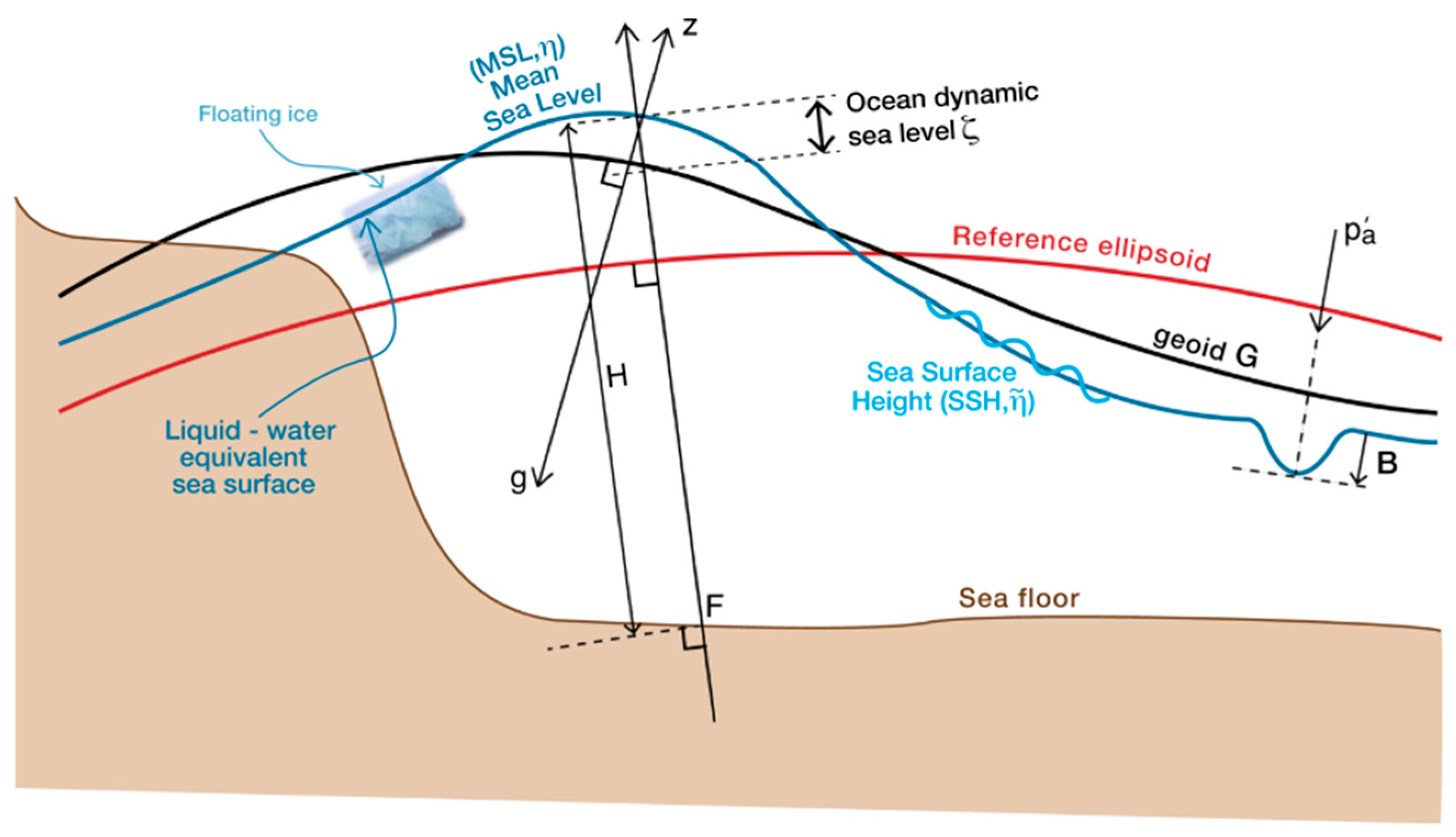
Disclaimer/Publisher’s Note: The statements, opinions and data contained in all publications are solely those of the individual author(s) and contributor(s) and not of MDPI and/or the editor(s). MDPI and/or the editor(s) disclaim responsibility for any injury to people or property resulting from any ideas, methods, instructions or products referred to in the content.

Article Metrics

Citations

Article Access Statistics

Multiple requests from the same IP address are counted as one view.