Data Recovery Methods for Sensor Data in Water Distribution Systems Based on Spatiotemporal Redundancy

Abstract

With the rapid development of smart water distribution systems, real-time monitoring data from large-scale sensor networks plays a critical role in system optimization and failure prediction. However, sensor data quality is often compromised by faults and missing values, which significantly undermine the reliability of decision-making. To address this issue, this study proposes a spatiotemporal redundancy-based data recovery method for sensor data. Specifically, polynomial fitting and hierarchical clustering are employed to analyze the spatiotemporal redundancy inherent in sensor data, based on which a weighted feature matrix is constructed. This matrix is then subjected to dimensionality reduction to enhance data representativeness. Five models—Multivariate Polynomial Regression, Holt-Winters, Long Short-Term Memory Sequence-to-Sequence, Multi-scale Isometric Convolution Network, and Transformer—were systematically compared in data recovery tasks. Experiments were conducted using real-world data from a water distribution system in China, involving 58 pressure sensors and 36 flow sensors. Results demonstrated that the developed method achieved high accuracy alongside efficient computation, particularly excelling in scenarios with abundant spatial redundancy.

1. Introduction

In the context of rapid urban expansion and the escalating demand for sustainable water services [1,2,3], modern Water Distribution Systems (WDSs) are undergoing a transformative shift towards intelligence [4,5]. This evolution is largely propelled by the integration of large-scale sensor networks, which continuously generate real-time data on parameters such as pressure, flow rate, and water quality [6,7,8]. These data streams are indispensable for a plethora of critical operations within WDSs. For instance, accurate pressure data enables the dynamic optimization of pump operations, thereby minimizing energy consumption and ensuring efficient water delivery [9,10]. Real-time flow monitoring, on the other hand, plays a pivotal role in the prompt detection of abnormal consumption patterns, which could be indicative of pipeline leaks or bursts [11,12].

Nevertheless, the integrity of sensor data in WDSs is frequently compromised by a multitude of factors [13,14]. Hardware malfunctions, such as sensor degradation or failure due to harsh environmental conditions (e.g., corrosion in wet environments), are common culprits. Additionally, electromagnetic interference from nearby electrical equipment or communication systems can corrupt data during transmission. 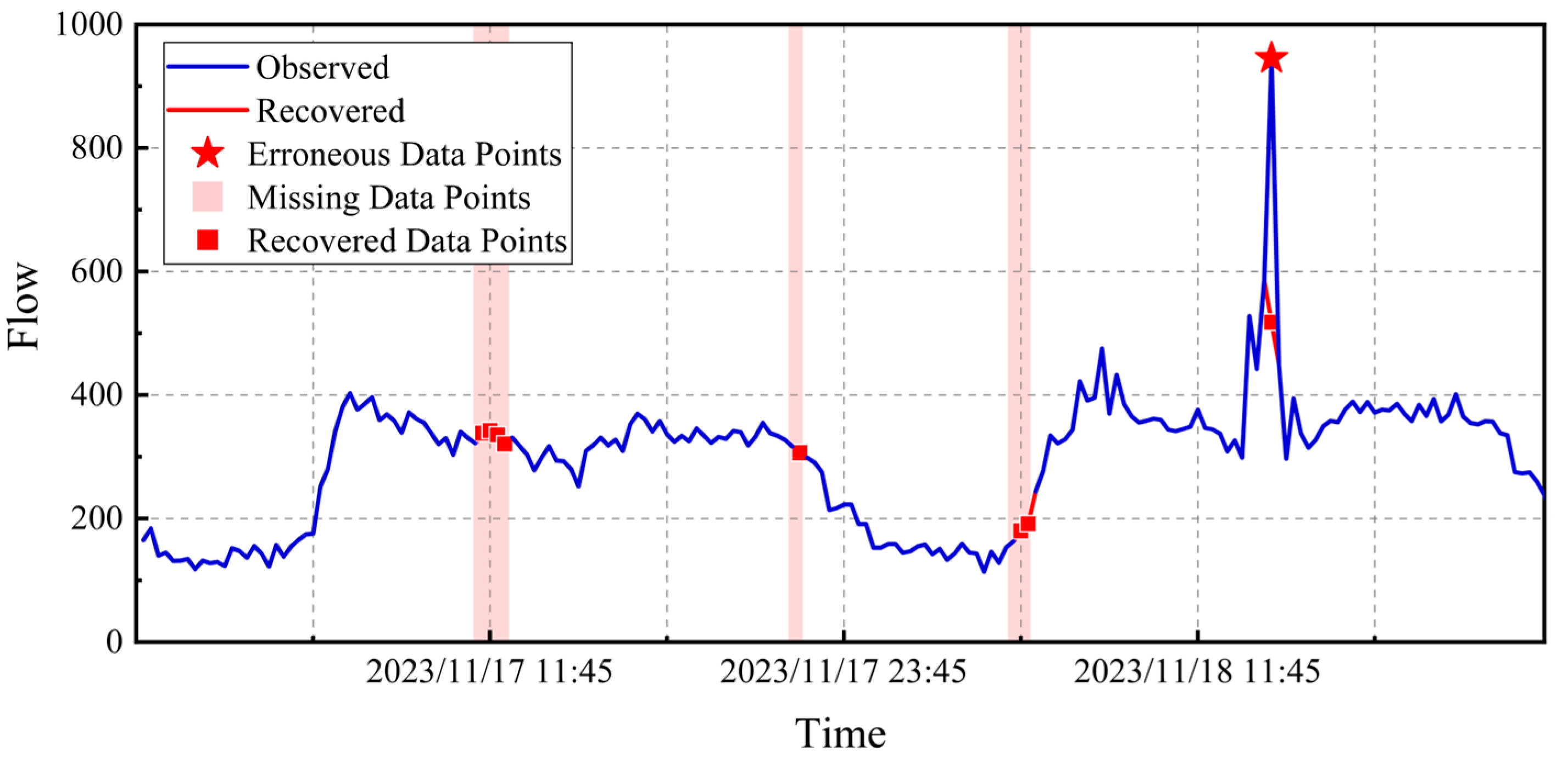Transmission losses, resulting from issues like network congestion or faulty communication protocols, also contribute to data gaps or inaccuracies [15,16]. These data anomalies are mainly of two types: missing data points, typically arising from temporary sensor outages or communication failures and illustrated by the red-shaded regions in Figure 1, and erroneous data points, caused by noise or miscalibration and marked by the red stars in Figure 1 [4]. Even minor data irregularities can have far-reaching consequences. For example, a single missing pressure reading might mask a significant drop in supply pressure, leading to delayed maintenance actions and potentially resulting in service disruptions for consumers [17].

Figure 1. Illustration of missing and erroneous data in water distribution system monitoring, highlighted by red-shaded regions and red star markers, respectively, along with their recovery results.

To mitigate the impact of these data quality issues, data recovery has emerged as a crucial preprocessing step in WDS monitoring [18]. Over the years, a diverse range of data recovery methods has been developed. Traditional approaches, such as linear regression and mean imputation, have been widely adopted due to their simplicity. Linear regression attempts to establish a linear relationship between variables to predict missing values [19]. However, as extensively documented in the literature, these methods are ill-suited to capture the intricate nonlinear relationships inherent in WDS data. WDS data is influenced by a complex interplay of factors, including hydraulic processes, user consumption behaviors, and network topologies, rendering it far from linearly correlated. Mean imputation, which replaces missing values with the mean of the available data, is equally simplistic. It fails to account for the temporal and spatial dependencies within the data, leading to suboptimal recovery results [20].

Time-series models, such as the Holt-Winters method, represent another category of traditional techniques. The Holt-Winters method is designed to capture both the trend and seasonality in time-series data and has found applications in various fields, including sales forecasting in retail [21].

In recent years, deep learning approaches have shown great promise in data recovery for WDSs. Models like Long Short-Term Memory (LSTM) networks [22,23] are capable of handling sequential data and capturing long-term dependencies. In the case of WDS data, they can learn the complex temporal patterns over extended periods, adapting to changes in water consumption patterns over months or even years. However, these deep learning models often require large datasets for practical training [24,25]. Gathering and preprocessing such extensive datasets can be challenging in real-world WDS scenarios, where data collection may be constrained by factors such as sensor availability, communication costs, and privacy concerns. Moreover, deep learning models demand substantial computational resources, which may not be practical for real-time monitoring systems that require immediate data recovery and analysis.

In WDSs, data recovery must consider not only temporal regularities—such as daily and weekly consumption cycles—but also spatial dependencies among hydraulically connected sensors. Yet existing approaches often fail to fully leverage this spatiotemporal redundancy. For example, Chu et al. [4] proposed a Bayesian fusion framework to calibrate nodal demands, which can address missing or anomalous data but ignores spatial correlations within the network. Jun et al. [11] demonstrated that historical mean imputation performs well for advanced metering infrastructure end-user demand data with pulse-like consumption patterns. However, such methods are less applicable to WDS telemetry, where pressure and flow signals exhibit strong inter-sensor dependencies driven by hydraulic connectivity. Zanfei et al. [18] assessed a range of imputation methods and highlighted their effects on urban water demand forecasting, but their analysis centered on downstream forecasting accuracy rather than on a recovery framework tailored to WDS data. More recently, Zhou et al. [26] introduced a graph-based imputation method grounded in graph signal sampling theory, which captures multi-level temporal correlations and performs well under continuous-missing conditions, but does not explicitly model spatial or topological relationships among multiple sensors. These shortcomings are echoed in the comprehensive survey by Osman et al. [27], which concluded that generic imputation techniques perform poorly under the strongly coupled spatiotemporal conditions of WDSs, reinforcing the need for domain-specific solutions.

A distinctive characteristic of WDS monitoring data is its inherent spatiotemporal redundancy, which, if systematically exploited, can substantially improve recovery accuracy. Temporal redundancy arises from the strong cyclicity of water consumption, while spatial redundancy stems from the hydraulic connectivity of pipelines, where adjacent sensors often display correlated fluctuations [28,29]. For instance, a pressure drop at one junction is likely to propagate downstream, creating predictable spatial patterns. Despite recent advances, current approaches still fail to integrate both temporal and spatial redundancies, underscoring the need for a unified feature representation that can support robust WDS data recovery.

Motivated by these limitations, this study systematizes and directly exploits the spatiotemporal redundancy inherent in WDS telemetry. We first quantify spatial correlations among sensors through segmented polynomial fitting and hierarchical clustering, and capture temporal redundancy by retrieving the most similar historical segments. Building on these, we construct a spatiotemporal redundancy matrix that integrates information from both other sensors and historical self-records, with correlation-based weighting and Principal Component Analysis (PCA) applied to reduce noise and highlight the most predictive features—without reliance on hydraulic models. Experiments on real-world data from a municipal WDS in China demonstrate that Multivariate Polynomial Regression achieves a favorable balance between accuracy and efficiency, making it particularly suitable for real-time deployment.

The remainder of this paper is structured as follows. Section 2 details the construction of spatiotemporal redundancy. Section 3 describes the feature engineering process. Section 4 introduces the data recovery models. Section 5 presents case studies and results. Section 6 concludes the study and outlines future work.

2. Construction of Spatiotemporal Redundancy

2.1. Data Correlation Assessment

The purpose of constructing spatiotemporal redundancy is to search for monitoring data sequences with similar variation trends for the current sequence of each sensor, thereby ensuring adequate data redundancy for recovery purposes.

The polynomial function is employed to fit time series data from water supply networks, aiming to capture periodic variation patterns in parameters such as water pressure and flow rate, and filter out random noise. For a given time series $f\left(t\right)$, its polynomial fitting function can be expressed by the following equation:

$$f\left(t\right)={\beta }_0+{\beta }_{1}t+{\beta }_2{t}^2+\cdots +{\beta }_p{t}^p,$$

(1)

where ${\beta }_0,{\beta }_1,{\beta }_2,\dots ,{\beta }_p$ are the polynomial fitting coefficients, and $p$ represents the polynomial fitting order.

Due to consumers’ habitual water usage patterns, the time series of water supply networks often exhibit strong diurnal periodicity. Therefore, segmented polynomial fitting is adopted to optimize coefficients within each segment, enabling effective capture of periodic variations while significantly reducing computational complexity. For a time series $i$ ($i=\{i_1,i_2,i_3\dots i_n\}$) containing $n$ cycles, the polynomial fitting function for any given cycle j can be expressed as follows:

$$f_j^i\left(t\right)={\beta }_0+{\beta }_{1}t+{\beta }_2{t}^2+\cdots +{\beta }_p{t}^p,t\in j.$$

(2)

For the polynomial fitting functions of two sequences $A$ and $B$ with the same time window, the correlation between them can be quantified using correlation coefficients. Given a time window $\{t_1,t_2,\dots ,t_m\}$ containing $m$ data points, the values of the two polynomial fitting functions are respectively:

$$F_A=\left. [f^A\left(t_1\right),f^A\left(t_2\right),\dots ,f^A\left(t_m\right)\right],$$

(3)

$$F_B=\left. [f^B\left(t_1\right),f^B\left(t_2\right),\dots ,f^B\left(t_m\right)\right].$$

(4)

The Pearson correlation coefficient is defined as the covariance between two vectors divided by the product of their standard deviations, calculated as follows:

$$r_{A,B}={\displaystyle \frac{{\sum }_{i=1}^m(f^A\left(t_i\right)-{\overline{f}}^A)(f^B\left(t_i\right)-{\overline{f}}^B)}{\sqrt{{\sum }_{i=1}^m{(f^A\left(t_i\right)-{\overline{f}}^A)}^2}\sqrt{{\sum }_{i=1}^m{(f^B\left(t_i\right)-{\overline{f}}^B)}^2}}},$$

(5)

where ${\overline{f}}^A$ and ${\overline{f}}^B$ represent the mean values of $F_A$ and $F_B$, respectively. The value range of $r_{AB}$ is $[-\mathrm{1,1}]$, with values approaching 1 indicating higher similarity in the variation trends of the two data sequences.

2.2. Spatial Redundancy Construction

By calculating the correlation coefficients between the current sequences of every two sensors, a correlation coefficient matrix $R$ is formed, which can be expressed as

$$R=\left. [\begin{array}{cccc}0& r_{12}& \cdots & r_{1q}\\ r_{21}& 0& \cdots & r_{2q}\\ ⋮& ⋮& \ddots & ⋮\\ r_{q1}& r_{q2}& \cdots & 0\end{array}\right].$$

(6)

In this matrix, the element $r_{ij}$ represents the correlation coefficient between sensor $i$ and sensor $j$, and $q$ denotes the number of sensors to be processed.

Next, hierarchical clustering is applied to group the current sensor sequences, where sensors with higher correlation coefficients are clustered together. The core step of hierarchical clustering involves merging clusters, where in each iteration, the two clusters with the smallest distance in the distance matrix $D$ are selected for merging.

Through hierarchical clustering, sensors with strong correlations are grouped together. Sensors within the same group exhibit similar variation trends in their data.

2.3. Temporal Redundancy Construction

The similarity between historical segments and the current segment of sensor data is identified through correlation coefficients, with the top $k$ most similar historical segments selected to construct temporal redundancy.

First, the current segment is defined as $Y$, and the historical time series of the sensor is divided into multiple subsequences $Y_j$. Next, the correlation coefficient $r(Y,Y_j)$ between the current segment $Y$ and each subsequence $Y_j$ is calculated, from which the $k$ subsequences with the smallest correlation distances are selected.

When the sensor group contains a sufficient number of sensors, it can be considered to possess adequate spatial data redundancy, thus allowing for relatively fewer historical subsequences to be selected. However, when the sensor count is low, greater reliance on temporal redundancy information becomes necessary. Therefore, the following Sigmoid function is introduced to automatically adjust the value of $k$:

$$k=⌈{\displaystyle \frac{10}{1+e^{0.1l}}}⌉,$$

(7)

where $l$ denotes the number of sensors in the corresponding sensor group.

2.4. Spatiotemporal Redundancy Construction

When data is missing from a particular sensor, the recovery value can be estimated by leveraging information from other sensors within the same group (spatial redundancy) or from its own historical records (temporal redundancy). Both types of redundant sequences are truncated to the same length as the current observation window (e.g., one day), and together they form the spatiotemporal redundancy matrix $M$, which serves as the basis for data recovery.

Specifically, let $Y_i$ denote the current data sequence of sensor $i$. The matrix $M$ is constructed as a multi-row structure, where the first row corresponds to $Y_i$, while the remaining rows consist of (a) the current sequences of other sensors in the same group and (b) the top-$l$ most similar historical subsequences of sensor $i$. Assuming that $M$ contains the time series of k other sensors and l historical subsequences, its dimension can be expressed as

$$M\in {\mathbb{R}}^{\left(k+l+1\right)\times N},$$

(8)

where $N$ is the window size (e.g., one day with 96 time steps). The resulting structure can be expressed as

$$M_N^i=\left. [\begin{array}{cccc}{y}_1^i& y_2^i& \cdots & y_N^i\\ y_1^{c_1}& y_2^{c_1}& \cdots & y_N^{c_1}\\ y_1^{c_2}& y_2^{c_2}& \cdots & y_N^{c_2}\\ ⋮& ⋮& \ddots & ⋮\\ y_1^{c_k}& y_2^{c_k}& \cdots & y_N^{c_k}\\ y_{j_1}^i& y_{j_1+1}^i& \cdots & y_{j_1+N-1}^i\\ y_{j_2}^i& y_{j_2+1}^i& \cdots & y_{j_2+N-1}^i\\ ⋮& ⋮& \ddots & ⋮\\ y_{j_l}^i& y_{j_l+1}^i& \cdots & y_{j_l+N-1}^i\end{array}\right].$$

(9)

Specifically, the first row represents the self-sequence, the second to $(k+1)$-th rows contain the group sequences, and the final $l$ rows correspond to the historical sequences. This unified representation explicitly integrates both spatial and temporal redundancy, providing a structured input for subsequent weighting and dimensionality reduction.

3. Extraction of Informative Spatiotemporal Features

The spatiotemporal redundancy matrix $M$ aggregates multiple time series from neighboring sensors and historical segments. While this fusion provides rich contextual information, it also introduces strong correlations, redundant patterns, and sensor noise. Directly inputting such raw multi-row data into recovery models can increase computational cost, amplify noise, and even degrade prediction accuracy due to multicollinearity. Therefore, it is necessary to refine $M$ into a compact and informative representation that highlights the most predictive signals while suppressing irrelevant redundancy. To achieve this, we adopt a progressive two-step process combining correlation-based weighting and PCA.

3.1. Correlation-Based Weighting

For each auxiliary time series (including other sensors and historical records of the target sensor), its relevance to the target sequence is quantified using the Pearson correlation coefficient. Intuitively, stronger correlations indicate higher predictive power. These coefficients are then used to form a diagonal weight matrix $W$ as follows:

$$W=\left. [\begin{array}{ccccc}1& 0& 0& \cdots & 0\\ 0& r_{M_1,M_2}& 0& \cdots & 0\\ 0& 0& r_{M_1,M_3}& \cdots & 0\\ ⋮& ⋮& ⋮& \ddots & ⋮\\ 0& 0& 0& \cdots & r_{M_1,M_{k+l+1}}\end{array}\right],$$

(10)

where $r_{M_1,M_j}$ represents the correlation coefficient between the first and the $j$-th row of $M$.

The weighted redundancy matrix $\widehat{M}$ is then obtained as:

$$\widehat{M}=WM.$$

(11)

This step effectively amplifies informative sequences that are highly correlated with the target while suppressing weakly related or redundant ones. As a result, the weighted matrix $\widehat{M}$ better captures the intrinsic spatiotemporal dependencies and reduces irrelevant interference.

3.2. PCA-Based Dimensionality Reduction

Although weighting reduces noise, $\widehat{M}$ may still contain redundant or correlated features—for instance, multiple pressure sensors or historical profiles often share similar dynamics. To further eliminate redundancy and obtain a more compact feature set, PCA is applied to the column-centered matrix $\widehat{M}$. The covariance matrix is computed as

$$C={\displaystyle \frac{1}{N-1}}{\widehat{M}}^T\widehat{M},$$

(12)

and then decomposed as

$$C=V\Lambda ({V)}^T.$$

(13)

In the formula, $V$ contains the eigenvectors, and $\Lambda$ is a diagonal matrix containing the eigenvalues. The top-ranked $a$ eigenvectors, explaining the majority of variance, are selected to form the matrix $V_a$. The original data is then projected onto the new principal component space, generating the reduced-dimensional feature matrix $F$ as

$$F=\widehat{M}{V}_a.$$

(14)

Together, correlation weighting and PCA form a concise and complementary process: the former emphasizes the most informative spatiotemporal features, while the latter compresses them into a compact, noise-free representation. The resulting feature matrix $F$ ensures robust and efficient data recovery, achieving a balanced trade-off between accuracy and computational cost in real-world WDS applications.

4. Data Recovery Model

Building upon the refined feature matrix $F$ derived in the previous section, this section evaluates multiple recovery models to reconstruct missing or anomalous sensor data. These models, ranging from traditional statistical and regression approaches to advanced deep learning frameworks, are used to examine how different learning paradigms exploit the extracted spatiotemporal features for accurate and efficient data recovery in WDSs.

4.1. Multivariate Polynomial Regression

Traditional data recovery methods mainly include linear regression and mean imputation [30], both of which fall under the category of linear models. Although widely used in practical engineering applications due to their simple implementation and high computational efficiency, these linear models exhibit significant limitations in data recovery processes. They assume a linear relationship between independent and dependent variables—an assumption that often fails in WDS, where monitoring data are typically influenced by multiple nonlinear factors. Consequently, linear regression models may fail to accurately depict the true relationship of data, resulting in low accuracy of data recovery results.

However, the extremely high computational efficiency of linear models gives them an advantage in real-time monitoring data processing for WDS. To overcome the limitations of traditional linear models, this paper focuses on a more advanced data recovery model, namely Multivariate Polynomial Regression (MPR), which provides a more effective solution for the recovery of missing and anomalous data. Compared with conventional linear regression, MPR can capture more complex nonlinear relationships in data while maintaining high computational efficiency, making it particularly suitable for practical applications in WDS. The MPR model utilizes the redundancy sequences in the feature matrix $F$ as multivariate independent variables to perform polynomial fitting on the target sensor data $Y$.

In practical implementation, the input matrix $Z$ is constructed through expansion of the feature matrix $F$, with its specific structure defined as follows:

$$Z=\left. [1,f_1,f_2,\dots ,f_{k+l},f_1^2,f_1{f}_2,f_2^2,\dots ,f_{k+l}^2,f_1^3,f_1^2{f}_2,\dots \right],$$

(15)

where, $f_j$ represents the $j$-th column of the feature matrix $F$. This expanded input matrix incorporates multiple polynomial orders and cross-feature interactions, enabling the model to capture more complex feature relationships.

The regression model can be expressed as

$$X=ZB+ϵ,$$

(16)

In this model, $B$ represents the vector of regression coefficients, and $ϵ$ denotes the error term.

The model is fitted using the least squares method, aiming to minimize the sum of squared residuals, which can be expressed as:

$$B=\arg \underset{B}{\min }‖X-{ZB‖}^2,$$

(17)

where, $‖\cdot ‖$ denotes the Euclidean norm.

The regression coefficients $\widehat{B}$ are obtained using the feature matrix preceding the data points to be recovered, and the recovered data values are calculated as follows:

$${\widehat{x}}_t=Z_t\widehat{B},$$

(18)

where ${\widehat{x}}_t$ represents the recovered value for the data point at time $t$, and $Z_t$ denotes the input matrix at time $t$.

MPR can effectively capture temporal dependencies in the data and relationships between features, significantly improving the accuracy of data recovery. Meanwhile, it retains the low computational complexity characteristic of linear models, providing a practical and easily implementable solution for real-time data recovery in WDS monitoring.

4.2. MICN

Convolutional Neural Networks (CNNs) initially achieved remarkable success in image processing and speech recognition, yet their architecture and principles can also be applied to variant models for time series forecasting. The Multi-scale Isometric Convolution Network (MICN) [31] is a novel CNN framework designed to enhance the capability of processing time series data. By employing multi-scale convolutional operations, MICN can simultaneously capture features of different frequencies in time series data, thus enhancing the model’s sensitivity to data variations. The design of MICN fully considers the characteristics of time series data, and realizes information extraction at different time scales using isometric convolution layers. This approach not only enhances the model’s representational capacity but also enables more flexible capture of complex data patterns.

4.3. Holt-Winters

Statistical methods have been widely applied in data recovery, especially when processing time series data. These methods typically apply statistical principles to predict missing values by analyzing trends, seasonality, and other patterns in the data. The Holt-Winters model, a classical statistical model for time series forecasting [21], extends the simple exponential smoothing method by modeling both trend and seasonal components. It consists of three core elements: level, trend, and seasonality. In WDS, sensor monitoring data usually exhibit clear seasonal patterns, making the Holt-Winters model particularly suitable.

When applying the Holt-Winters model, the initialization step is performed first. This involves decomposing the time series into the level component ($L_0$), trend component ($T_0$), and seasonal component ($S_{t-b}$, where $b$ denotes the season length). Subsequently, these components are updated sequentially through the level component, trend component, and seasonal component.

Although the Holt-Winters model performs well in capturing trends and seasonality in time-series data, it has a significant limitation in this study. Since the feature matrix $F$ in this study expands the time series of a single sensor to form a multivariate dataset, while the Holt-Winters model only handles univariate time series. Therefore, this model can only utilize temporal redundancy described in this paper for data recovery, and fails to leverage spatial redundancy. This limitation considerably restricts its predictive capability in complex data environments.

4.4. LSTMs2s

Long Short-Term Memory (LSTM) networks are among the most widely used deep learning models for time series analysis and forecasting [22]. Owing to their ability to effectively capture the long-term and short-term dependencies in time series data, LSTMs have been extensively employed in the prediction and anomaly detection of WDS sensor data [32]. Given their demonstrated proficiency in processing univariate time series data, researchers have increasingly explored their application to complex multivariate time series forecasting tasks.

The LSTMs2s (LSTM sequence-to-sequence) [33] framework adopted in this study is a variant of LSTM, specifically optimized for multivariate time series forecasting. By introducing an encoder–decoder architecture, LSTMs2s enhances the native LSTM’s capability in processing output sequences, making it more suitable for other sequence generation tasks. Distinct from conventional LSTM models used in WDS, the feature matrix $F$ utilized in this paper is a data matrix that projects temporal and spatial dimensions onto the principal component space at the same scale. This construction method is different from the traditional approach of constructing LSTM input datasets in chronological order. By integrating historical and real-time data from multiple sensors, the $F$ data matrix can more comprehensively reflect the dynamic characteristics of the system, thereby improving the data recovery effect.

4.5. Transformer

The Transformer model [34] is an extremely popular deep learning architecture in recent years, particularly serving as the foundation for the success of large language models. Its core mechanism is based on the self-attention mechanism, which significantly improves computational efficiency by processing input sequences in parallel and overcomes the limitations of traditional Recurrent Neural Networks (RNNs) when handling long-sequence data. For time series data recovery, the Transformer architecture can flexibly model both long- and short-term dependencies in the data. Through the self-attention mechanism, the model dynamically adjusts its focus on the importance of different time points, thereby enabling more accurate predictions. The Transformer’s powerful capability in processing multivariate data is especially well-suited to the data structure of the feature matrix F described in this paper, making it an ideal choice for data recovery.

5. Case Study and Results

5.1. Dataset Description

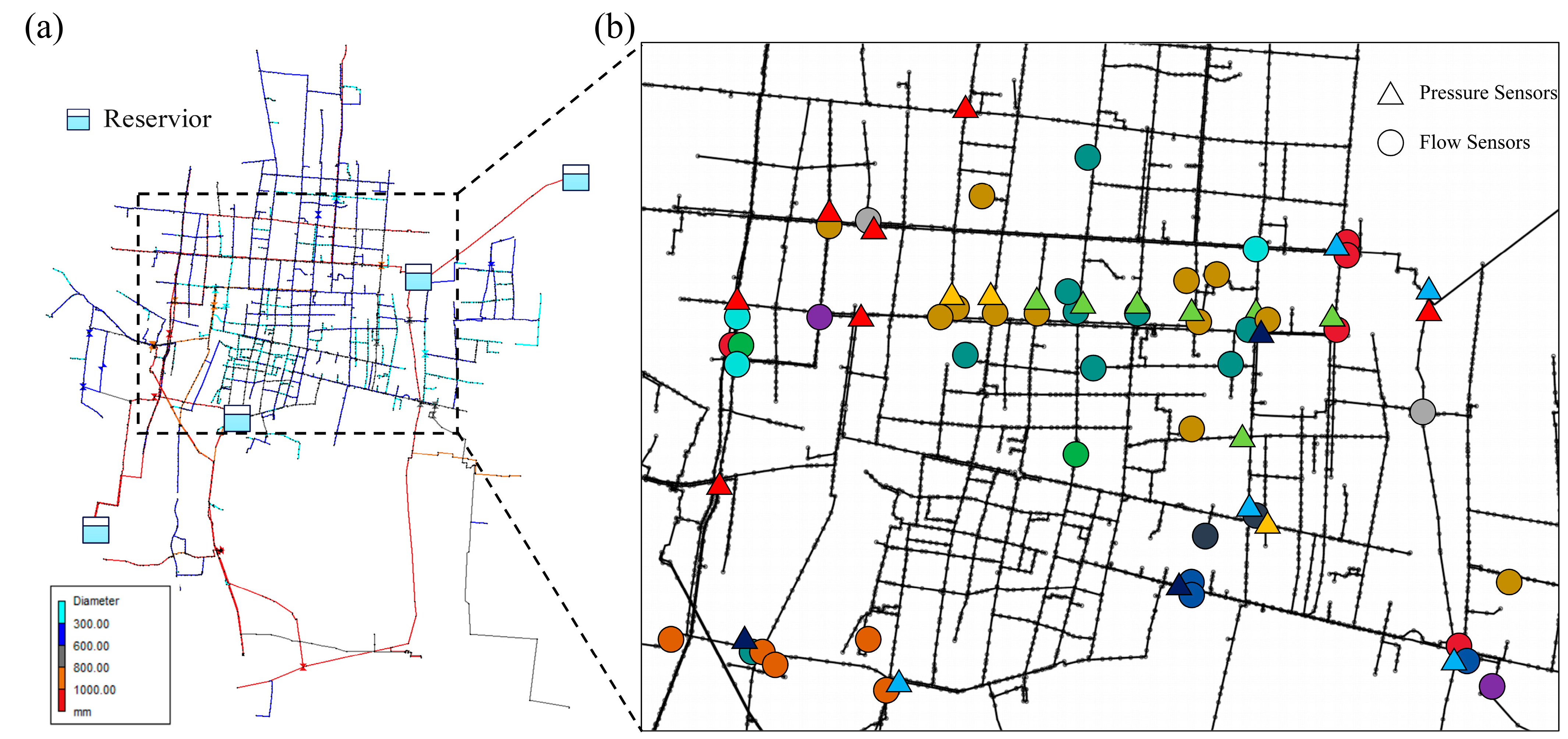
We validate the proposed recovery framework on a real-world WDS dataset comprising 72 pressure sensors and 49 flow sensors. As shown in Figure 2a, the studied network belongs to a medium-sized city, supplied by several reservoirs via booster pumping, and includes approximately 4350 km of mains and 4100 nodes; pipe colors indicate diameters. Figure 2b depicts the sensor deployment and grouping in the urban area: circles denote pressure sensors and triangles denote flow sensors; sensors with the same color are clustered into the same group.

Figure 2. Topology of the water distribution network and grouped sensor deployment. (a) Schematic of the water distribution network topology showing pipe diameters and reservoir locations. (b) Spatial distribution and grouping of sensors in the urban area, where circles represent pressure sensors and triangles represent flow sensors. Sensors with the same color belong to the same group.

Sensor locations were determined by the water utility’s engineering team according to hydraulic representativeness and operational accessibility. In practice, pressure sensors are mainly installed on distribution mains at key or terminal junctions, while flow sensors are placed on transmission mains, DMA inlets/outlets, and entrances to major demand areas (e.g., industrial parks).

All sensors report at 15-min intervals. Considering that water pressure and flow in WDSs generally exhibit daily periodic variations [14], the sliding window size was set to one day (96 data points) to capture complete diurnal patterns. The dataset used in this study contains monitoring records collected from April 2023 to April 2024.

For data quality control, outliers were identified using the 3σ rule and treated as missing for subsequent imputation. The raw missing rates were approximately 9.5% for pressure data and 18.4% for flow data. In addition, sensors exhibiting severe malfunctions over extended periods (e.g., continuous data loss or constant readings lasting longer than one week) or those with an overall missing rate exceeding 25% were excluded from the dataset to ensure reliability. After this screening process, a total of 58 pressure sensors and 36 flow sensors were retained for analysis. Following data cleaning, the overall missing rates were reduced to 4.8% for pressure and 6.2% for flow.

Due to the unavailability of maintenance or work-order logs, periods affected by repairs, bursts, or emergency interventions were not separately analyzed and were thus excluded from the scope of this study.

5.2. Sensor Grouping in the Case Study WDS

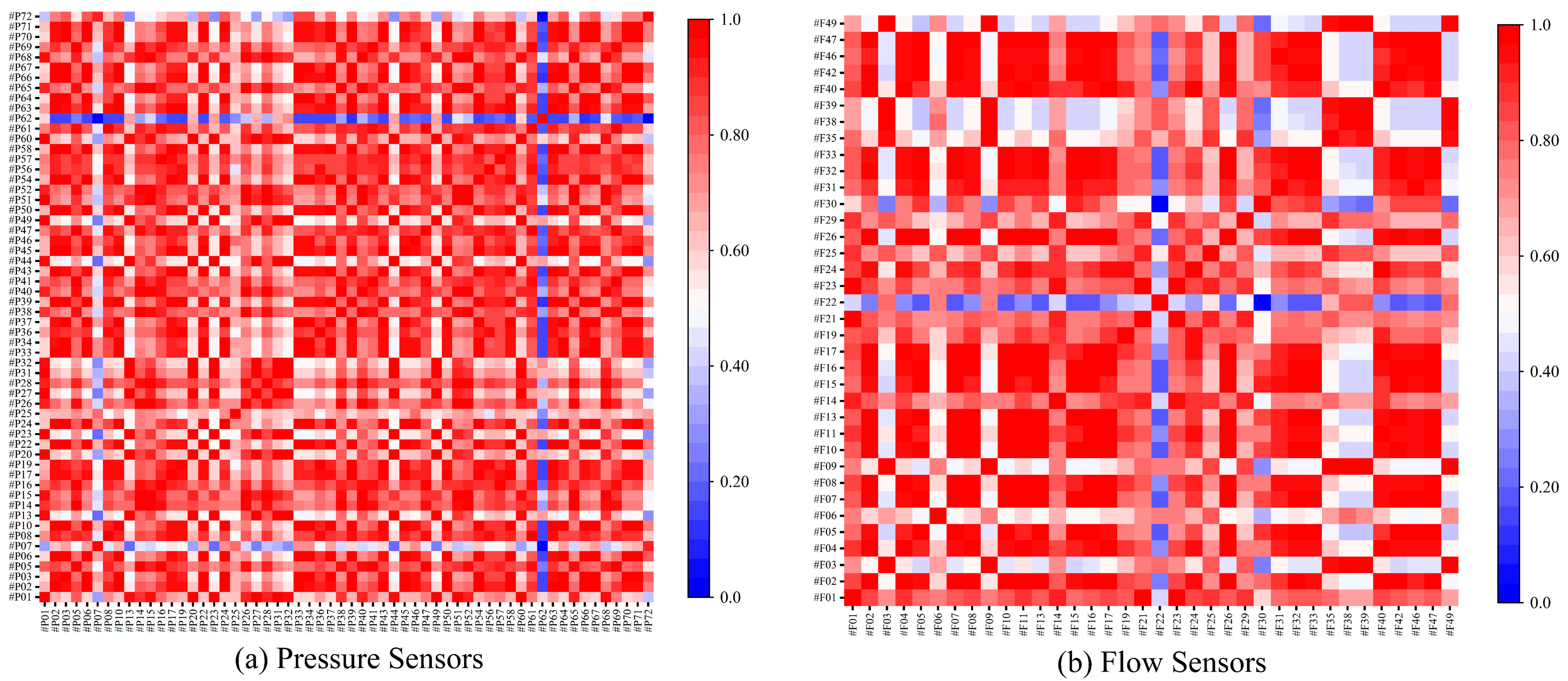
The Pearson correlation coefficient was used to quantify pairwise relationships among sensors, forming a distance matrix $D$. In this study, pressure and flow sensors are denoted as #P and #F, respectively (e.g., #P01 represents pressure sensor #01, and #F01 represents flow sensor #01). Figure 3 visualizes the temporal correlation between every two pressure or flow sensors in the network.

Figure 3. Correlation heatmaps among (a) pressure sensors and (b) flow sensors in the case study WDS. The symbol “#” denotes the sensor index (e.g., #P01 and #F01 represent pressure and flow sensors, respectively).

As shown in Figure 3a, several pressure sensors (e.g., #P62) display consistently high correlations with many others, indicating that these sensors share similar temporal variation patterns. Conversely, some sensors exhibit weaker correlations, suggesting isolated locations or distinct hydraulic conditions. This high-dimensional correlation structure not only captures inter-sensor dependencies but also reflects intra-sensor temporal coherence, demonstrating the robustness of the data and the reliability of the monitoring system.

Based on the distance matrix $D$, hierarchical clustering was applied to group sensors with similar temporal behaviors. Both pressure and flow sensors were clustered separately and re-evaluated every two days to account for evolving network dynamics. The final grouping results are shown in Table 1, consistent with the spatial distribution displayed in Figure 2b.

Table 1. Grouping results of pressure and flow sensors in the case study WDS.

Groups	Sensor	Groups	Sensor	Groups	Sensor	Groups	Sensor
#Group 1	#P01 #P20 #P60	#Group 6	#P15 #P51 #P68	#Group 11	#P41 #P57 #P69	#Group 17	#F03 #F09 #F22 #F35 #F38 #F39 #F49
#Group 2	#P02 #P10 #P22 #P39 #P43 #P45 #P46 #P50 #P54 #P58 #P66 #P71	#Group 7	#P13 #P23 #P27 #P44 #P49	#Group 12	#P14 #P26 #P38 #P40 #P65
		#Group 8	#P03 #P06 #P24 #P33 #P34 #P37 #P64 #P72	#Group 13	#F01 #F21 #F23	#Group 18	#F07 #F10 #F13 #F16 #F26 #F32 #F42 #F47
				#Group 14	#F24 #F40
#Group 3	#P05 #P16	#Group 9	#P19 #P36	#Group 15	#F02 #F04 #F08 #F11 #F17 #F19	#Group 19	#F05 #F15 #F33
#Group 4	#P17 #P63
#Group 5	#P31 #P32	#Group 10	#P47 #P61	#Group 16	#F28 #F52	#Group 20	#F31 #P46

Note: #P and #F denote pressure and flow sensors respectively.

From the clustering results, groups vary in size—for instance, some pressure groups contain more than 10 sensors, while others have only 2. This imbalance reflects the heterogeneous layout of the network, where densely connected trunk regions exhibit stronger correlations, while peripheral or industrial zones show greater diversity. Such grouping provides valuable prior knowledge for subsequent analyses, as sensors within the same group can serve as redundancy sources for each other during data recovery.

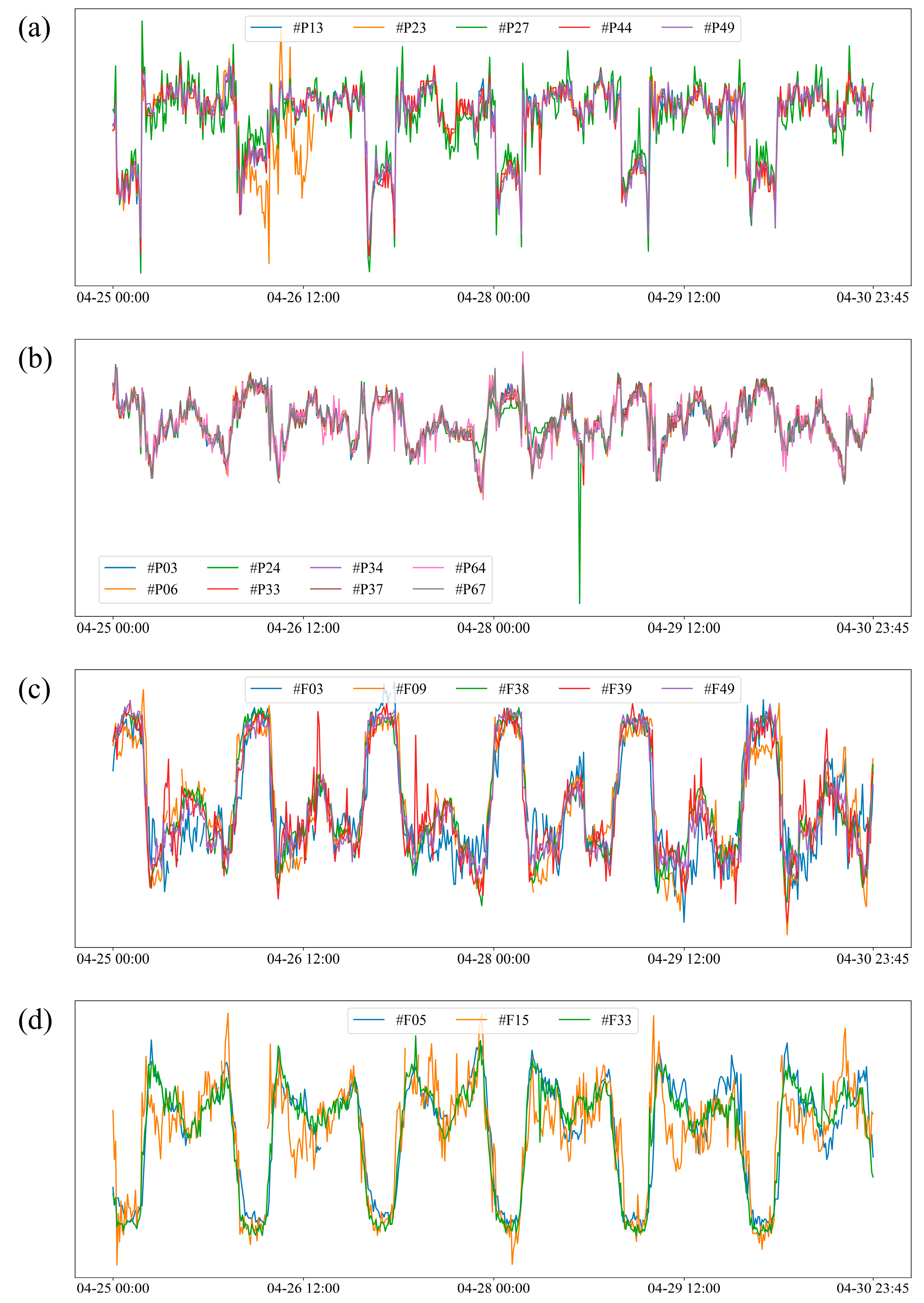
Figure 4 illustrates representative temporal sequences from four groups (pressure groups 7 and 8, flow groups 17 and 19). Sensors within the same group exhibit highly consistent variation trends, confirming the effectiveness of the grouping method. For example, in Figure 4a, sensor #P23 shows a sudden deviation around 26 April 12:00, differing from other sensors in its group—a sign of possible anomalies or local disturbances. Similarly, in Figure 4b, flow sensor #F24 shows an extreme short-lived spike compared with its group peers. These cases highlight the potential of sensor grouping to support anomaly detection and improve the interpretability of monitoring data.

Figure 4. Representative monitoring time series of sensor groups in the case study WDS: (a) Group 7 and (b) Group 8 for pressure sensors; (c) Group 17 and (d) Group 19 for flow sensors.

5.3. Results of the Proposed MPR Method

To evaluate the effectiveness of the proposed MPR model, experiments were conducted using the real-world WDS dataset described in Section 5.1. The cleaned and imputed data were used to ensure reliable model training. To simulate real-time recovery, the most recent 960 time points (equivalent to 10 days) were selected as the test set, where the corresponding observations were intentionally masked and treated as missing. For each missing point, the associated feature matrix at that time was input into the MPR model for recovery. The recovered values were then compared with the original observations to assess reconstruction accuracy.

L2 regularization was introduced to control model complexity and enhance both robustness and generalization capability. Data from the 10 days preceding the recovery point (a total of 960 data points) was selected as the validation set to tune the parameters of the MPR model. A grid search was performed on the validation set to optimize four parameters: the L2 regularization coefficient $\alpha$, the input step size $n$, the polynomial fitting order $p$, and the number of principal components $m$. The input step size $n$ corresponds to the number of columns in the input feature matrix $F$, while the number of principal components $m$ corresponds to the number of rows in the input feature matrix $F$. In the grid search, the candidate values for the $\alpha$ were 0.001, 0.01, 0.075, 0.25, 0.5, and 0.9; the $m$ ranged from 1 to the maximum possible; the $n$ ranged from 1 to 15; and the $p$ ranged from 1 to 4. The objective of the grid search was to minimize the mean squared error (MSE) between the recovered values and the true values in the validation set. Table 2 presents the optimal parameter combination for each sensor obtained from the grid search results.

Table 2. Optimal combinations of MPR data recovery parameters for different sensors obtained from the grid search.

Sensor	$\mathit{\alpha }$	$\mathit{m}$	$\mathit{n}$	$\mathit{p}$	Sensor	$\mathit{\alpha }$	$\mathit{m}$	$\mathit{n}$	$\mathit{p}$
#F01	0.001	2	4	1	#P01	0.001	2	13	1
#F02	0.5	3	2	2	#P02	0.075	10	5	1
#F03	0.01	5	3	2	#P03	0.001	3	3	2
#F04	0.001	9	4	1	#P05	0.001	1	3	3
#F05	0.9	4	5	3	#P06	0.001	1	5	3
#F06	0.9	1	3	3	#P07	0.9	2	1	3
#F07	0.01	11	2	1	#P08	0.075	4	1	3
#F08	0.001	7	6	1	#P10	0.001	4	1	3
#F09	0.001	7	3	2	#P13	0.075	1	3	3
#F10	0.001	11	9	1	#P14	0.001	3	5	1
#F11	0.001	7	4	1	#P15	0.001	3	3	1
#F13	0.001	11	4	1	#P16	0.001	4	9	1
#F14	0.01	1	5	3	#P17	0.001	4	6	1
#F15	0.001	2	4	3	#P19	0.9	1	6	2
#F16	0.01	11	5	1	#P20	0.001	3	2	3
#F17	0.001	3	2	3	#P22	0.001	4	6	1
#F19	0.075	3	2	3	#P23	0.25	1	2	3
#F21	0.001	3	3	2	#P24	0.001	12	6	1
#F22	0.001	7	2	2	#P25	0.001	4	1	3
#F23	0.001	1	9	2	#P26	0.001	8	3	1
#F24	0.25	1	3	3	#P27	0.001	3	8	1
#F25	0.075	1	1	3	#P28	0.25	1	2	3
#F26	0.001	5	3	2	#P31	0.001	2	1	3
#F29	0.001	4	6	1	#P32	0.001	1	5	2
#F30	0.01	1	15	1	#P33	0.01	3	6	2
#F31	0.5	2	3	2	#P34	0.001	3	1	3
#F32	0.001	1	3	3	#P36	0.001	1	5	2
#F33	0.001	2	5	3	#P37	0.001	7	2	1
#F35	0.001	3	4	2	#P38	0.001	2	2	2
#F38	0.001	5	3	2	#P39	0.001	7	1	2
#F39	0.075	7	12	1	#P40	0.001	3	3	2
#F40	0.9	1	5	3	#P41	0.001	2	2	3
#F42	0.001	7	3	2	#P43	0.01	15	1	1
#F46	0.9	2	5	1	#P44	0.001	2	2	3
#F47	0.001	5	3	2	#P45	0.001	10	4	1
#F49	0.001	5	3	2	#P46	0.001	4	8	1
#P62	0.25	1	2	3	#P47	0.01	5	7	1
#P63	0.001	1	3	3	#P49	0.001	4	1	3
#P64	0.075	5	1	3	#P50	0.001	4	1	2
#P65	0.001	2	3	1	#P51	0.001	2	2	3
#P66	0.001	7	2	2	#P52	0.9	1	3	3
#P67	0.075	3	1	2	#P54	0.001	7	5	1
#P68	0.001	1	2	3	#P56	0.5	2	9	1
#P69	0.001	3	2	2	#P57	0.001	4	9	1
#P70	0.001	1	8	1	#P58	0.01	15	1	1
#P71	0.001	1	3	1	#P60	0.01	1	4	1
#P72	0.001	3	5	2	#P61	0.001	2	1	1

Note: #P and #F denote pressure and flow sensors respectively.

As shown in Table 2, during the data recovery process, sensors with different data characteristics exhibit substantial variations in the selection of regularization coefficients, input step sizes, polynomial fitting orders, and numbers of principal components. This experimental finding confirms the importance of selecting appropriate processing parameters based on the data characteristics of individual sensors when performing monitoring data recovery in WDS. It also indicates the sensitivity of MPR recovery performance to parameter selection. Nevertheless, as a linear model, MPR offers computational efficiency that is difficult for other nonlinear approaches to match, and therefore conducting grid search or other parameter optimization methods does not impose a significant computational burden.

After obtaining the optimal MPR parameters for each sensor, a single-step data recovery experiment of 960 steps was conducted. The recovery accuracy of the MPR method was evaluated using the Mean Squared Error (MSE) and Mean Absolute Error (MAE). The experimental results are presented in Table 3, from which it can be observed that MPR achieves extremely high accuracy (MSE < 0.3) in the data recovery tasks for most sensors.

Table 3. Data recovery accuracy of the 960-step single-step experiment using MPR.

Sensor	MSE	MAE	Sensor	MSE	MAE	Sensor	MSE	MAE
#P01	0.003	0.040	#P41	0.149	0.287	#F05	0.061	0.185
#P02	0.102	0.239	#P43	0.361	0.500	#F06	0.244	0.219
#P03	0.043	0.158	#P44	0.166	0.275	#F07	0.021	0.104
#P05	0.268	0.370	#P45	0.084	0.207	#F08	0.062	0.184
#P06	0.185	0.326	#P46	0.451	0.527	#F09	0.044	0.156
#P07	0.300	0.289	#P47	0.247	0.351	#F10	0.113	0.221
#P08	0.666	0.578	#P49	0.060	0.166	#F11	0.017	0.099
#P10	0.070	0.178	#P50	0.084	0.189	#F13	0.007	0.063
#P13	0.038	0.131	#P51	0.111	0.256	#F14	0.388	0.452
#P14	0.126	0.267	#P52	0.729	0.607	#F15	0.147	0.291
#P15	0.112	0.254	#P54	0.057	0.167	#F16	0.006	0.057
#P16	0.619	0.584	#P56	0.570	0.579	#F17	0.019	0.090
#P17	0.209	0.358	#P57	0.516	0.583	#F19	0.083	0.162
#P19	0.544	0.518	#P58	0.052	0.175	#F21	0.277	0.403
#P20	0.421	0.435	#P60	0.002	0.034	#F22	0.080	0.188
#P22	0.062	0.187	#P61	0.196	0.321	#F23	0.560	0.555
#P23	0.115	0.216	#P62	0.217	0.103	#F24	0.167	0.272
#P24	0.158	0.230	#P63	0.189	0.327	#F25	0.266	0.257
#P25	0.244	0.131	#P64	0.142	0.277	#F26	0.011	0.072
#P26	0.095	0.225	#P65	0.277	0.378	#F29	0.371	0.447
#P27	0.130	0.271	#P66	0.106	0.233	#F30	0.415	0.449
#P28	0.689	0.473	#P67	0.055	0.179	#F31	0.327	0.386
#P31	0.495	0.512	#P68	0.175	0.296	#F32	0.072	0.183
#P32	0.886	0.687	#P69	0.146	0.283	#F33	0.037	0.142
#P33	0.063	0.188	#P70	0.988	0.747	#F35	0.047	0.166
#P34	0.057	0.167	#P71	0.143	0.233	#F38	0.023	0.115
#P36	1.089	0.661	#P72	0.082	0.212	#F39	0.075	0.202
#P37	0.050	0.170	#F01	0.241	0.365	#F40	0.037	0.113
#P38	0.268	0.387	#F02	0.223	0.336	#F42	0.008	0.063
#P39	0.145	0.286	#F03	0.065	0.198	#F46	0.138	0.163
#P40	0.359	0.453	#F04	0.035	0.118	#F47	0.004	0.049

Note: #P and #F denote pressure and flow sensors respectively.

Next, an ablation experiment was conducted to evaluate the contribution of each process in the feature matrix construction to the MPR data recovery performance. The key processes include spatial redundancy construction, temporal redundancy construction, MIC-based normalization, and PCA-based dimensionality reduction. By comparing the data recovery performance across five datasets, including $F$ (full process), $F-NS$ (without spatial redundancy), $F-NT$ (without temporal redundancy), and $F-NP$ (without principal component analysis), the contribution of each processing step to the recovery performance was assessed. The results of the dissolution experiment are presented in Table 4.

Table 4. Data recovery accuracy of the dissolution experiment using MPR.

Dataset Construction		Pressure Sensors	Flow Sensors
$F$	MSE	0.258	0.131
	MAE	0.318	0.212
$F-NS$	MSE	0.606 (135%)	0.216 (65%)
	MAE	0.502 (58%)	0.265 (25%)
$F-NT$	MSE	0.446 (73%)	0.291 (122%)
	MAE	0.401 (26%)	0.335 (58%)
$F-NP$	MSE	0.531 (106%)	0.214 (63%)
	MAE	0.443 (39%)	0.254 (20%)

Note: Values in parentheses indicate the reduction ratio compared with the full process.

As shown in Table 4, the accuracy of data recovery varies with the method used to construct the input data matrix, and the dependency patterns differ across sensor types. Pressure sensors rely more heavily on spatial redundancy, whereas flow sensors depend more on temporal redundancy. Moreover, pressure sensors exhibit greater sensitivity to feature extraction techniques such as PCA, indicating a higher dependence on feature engineering. These findings validate the adaptability of the proposed feature matrix construction method, which can flexibly leverage effective data redundancy to accommodate sensors with different data characteristics in WDS, thereby achieving high data recovery accuracy.

5.4. Model Comparison

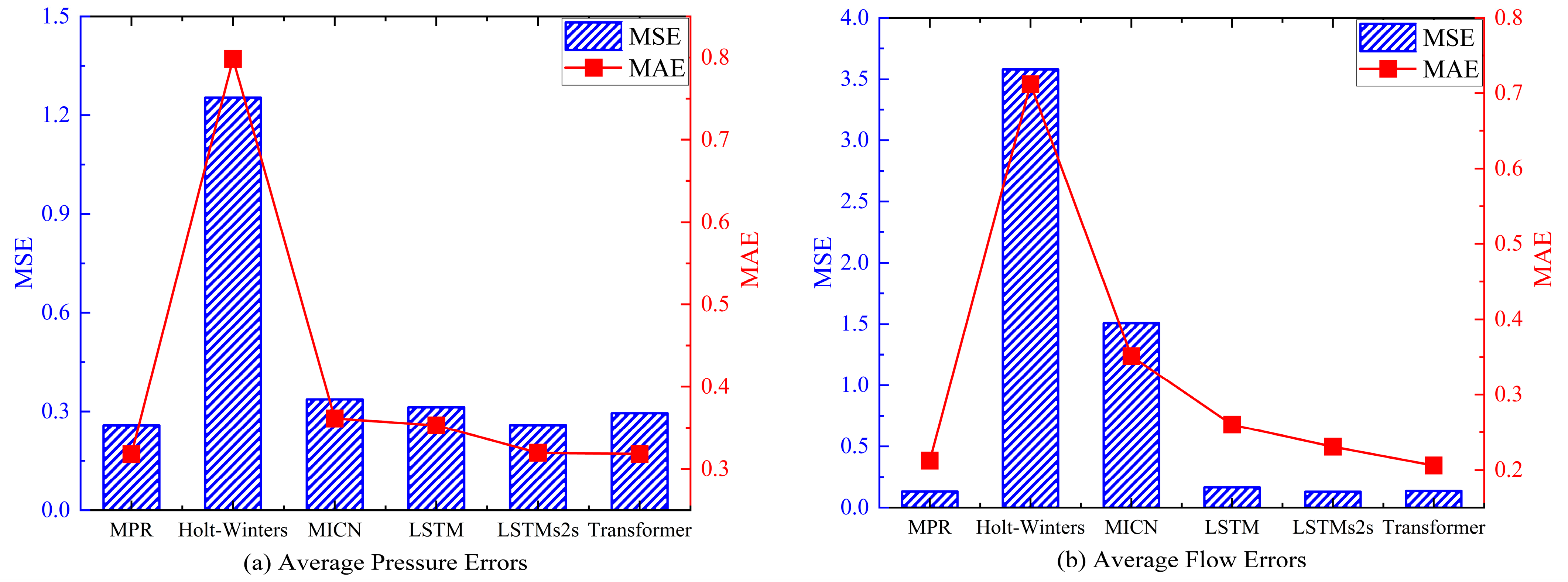
A systematic comparison of data recovery performance was conducted across six representative models by computing the MSE and MAE for both pressure and flow sensors. The experimental design was consistent with that described in Section 5.3, using a 960-step single-point recovery setup. For deep learning models including MICN, LSTM, LSTMs2s, and Transformer, the hyperparameters were tuned for stable convergence, with a learning rate of 0.001, batch size of 32, dropout rate of 0.9, and early stopping at 15 epochs.

As shown in Figure 5, the proposed MPR model consistently ranks among the top-performing methods across both pressure and flow sensors, achieving the lowest or near-lowest errors in most cases. This advantage primarily stems from its ability to exploit spatial–temporal redundancy and adaptively extract correlated features through polynomial regression and normalization.

Figure 5. Comparative performance of different models in data recovery experiments, in terms of average MSE and MAE for (a) pressure and (b) flow sensors.

In contrast, Holt–Winters exhibits the weakest performance across both datasets, highlighting the inherent limitation of univariate time-series models that fail to leverage spatial correlations or multivariate dependencies. MICN performs moderately well but struggles to capture non-stationary flow fluctuations, leading to higher MSE in flow recovery. LSTM achieves stable yet sub-optimal results due to its reliance on temporal recurrence without explicit spatial modeling, whereas LSTMs2s introduces a more flexible sequence-to-sequence structure that improves temporal learning but still lacks spatial feature coupling.

Among neural architectures, the Transformer demonstrates strong generalization, particularly in flow recovery, benefiting from its global attention mechanism that effectively captures long-range dependencies. Nevertheless, it remains less efficient than MPR in reconstructing smooth pressure variations, likely because attention models are less sensitive to small-scale fluctuations under limited data.

Overall, MPR consistently outperforms both traditional statistical and deep learning approaches, achieving higher accuracy across different sensor types while maintaining lower computational complexity. These results confirm that leveraging multi-source redundancy and local feature normalization enables MPR to balance interpretability and precision in real-world WDS recovery tasks.

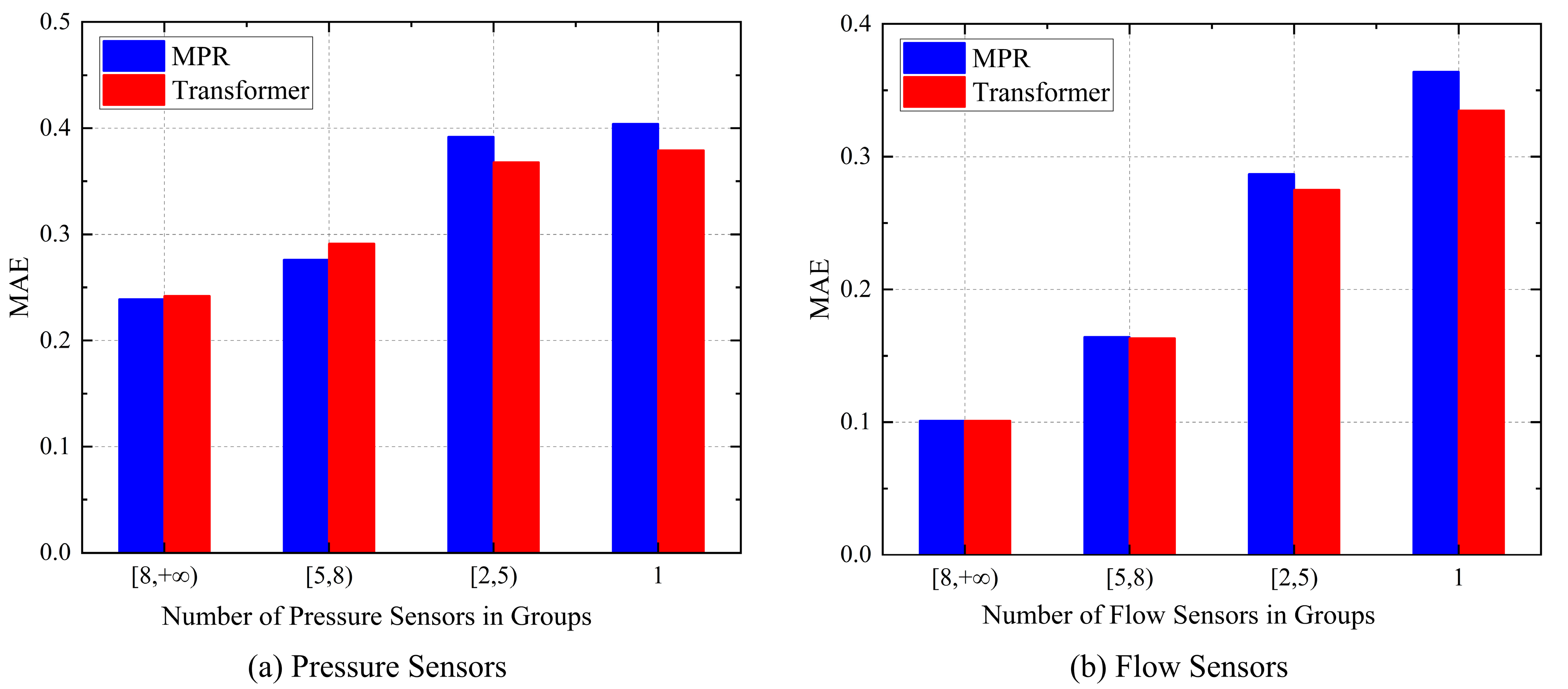
To further examine how model performance varies under different spatial redundancy conditions, we compared the two best-performing models identified in the preceding comparison—MPR and Transformer. These models were selected because MPR consistently achieved the lowest or near-lowest errors across both sensor types, while Transformer demonstrated outstanding performance among deep learning architectures.

Table 5 presents the MSE of data recovery experiments under varying numbers of sensors within spatial redundancy groups. The findings indicate that in groups with a larger number of sensors, the MPR model significantly outperforms the Transformer model in data recovery accuracy; conversely, when the number of sensors is smaller, the Transformer model demonstrates superior recovery performance. This observation suggests that extended linear models such as MPR can achieve effective data recovery when the feature matrix contains abundant spatial redundancy. In contrast, deep learning models exhibit stronger temporal modeling capabilities based on historical data when spatial redundancy is limited and modeling must rely more heavily on temporal redundancy. Based on these findings, linear models could be used when sensor groups are large, while deep learning models could be favored when sensor groups are small. Such a strategy could serve as a practical solution in engineering applications.

Table 5. Average errors of data recovery experiments within different sensor groups.

Groups	Sensor	MAE		Groups	Sensor	MAE
		MPR	Transformer			MPR	Transformer
#Group 8	#P03	0.158	0.161	#Group 18	#F07	0.104	0.196
	#P06	0.326	0.333		#F10	0.221	0.216
	#P24	0.230	0.239		#F13	0.063	0.058
	#P33	0.188	0.195		#F16	0.057	0.055
	#P34	0.167	0.173		#F26	0.072	0.072
	#P37	0.170	0.170		#F32	0.183	0.182
	#P64	0.277	0.299		#F42	0.063	0.065
	#P72	0.212	0.235		#F47	0.049	0.048
#Group 6	#P15	0.254	0.223	#Group 13	#F01	0.365	0.359
	#P51	0.256	0.222		#F21	0.403	0.393
	#P68	0.296	0.293		#F23	0.555	0.529
#Group 3	#P05	0.370	0.340	#Group 14	#F24	0.272	0.270
	#P16	0.584	0.560		#F40	0.113	0.110

Note: The symbol “#” denotes the index of each sensor group.

To validate this observation in more detail, the statistical results in Figure 6 provide a deeper validation of the aforementioned strategy. The results indicate that although both the MPR and Transformer models experience a decline in data recovery performance as the number of sensors decreases, the MPR model is more sensitive to changes in sensor quantity, exhibiting a more pronounced performance drop. In contrast, the Transformer model’s performance degradation is comparatively smaller. Additionally, for pressure sensor data recovery, the Transformer model’s accuracy is significantly lower than that of the MPR model. In contrast, for flow sensor data recovery, the Transformer model outperforms the MPR model. These findings highlight the significant differences in model performance across different sensor types, suggesting that appropriate model selection should be based on the specific application context.

Figure 6. Average MAE of MPR and Transformer models under varying sensor group sizes for (a) pressure and (b) flow data recovery.

5.5. Computational Efficiency and Practical Feasibility

In real-time monitoring and management of water distribution systems (WDS), the computational efficiency of data recovery models is a critical factor determining their practical applicability. If the data recovery module requires excessive computation time before subsequent decision-making or control tasks can proceed, its practical utility in real-time applications will be substantially diminished. Therefore, Figure 7 reports the model training time and the average time required for single-step data recovery under a standardized experimental environment equipped with an Intel 12th-Gen i7 CPU (Intel Corporation, Santa Clara, CA, USA) and an RTX 3060 Laptop GPU (NVIDIA Corporation, Santa Clara, CA, USA).

Figure 7. Model training time and average per-step recovery time in data recovery experiments.

As shown in Figure 7, the proposed MPR model exhibits remarkably high computational efficiency, requiring only 0.0158 s for training and 0.0008 s for each recovery step—several orders of magnitude faster than deep learning models. In comparison, Transformer and LSTM-based architectures incur substantially higher computational costs, with training times of 825.4 s and 153.7 s, respectively. Although these deep models achieve competitive accuracy, their extensive parameter tuning and iterative optimization processes lead to significant time overheads, which may hinder their deployment in real-time WDS operations.

Traditional statistical methods such as Holt–Winters require minimal data representation learning, resulting in shorter training time than neural networks, but they still consume more time than MPR due to the need for repeated smoothing and recursive calculations at each recovery step. Among the deep models, MICN and LSTMs2s demonstrate relatively moderate computational costs compared with Transformer, yet they remain two to three orders of magnitude slower than MPR.

These results collectively demonstrate that the MPR framework achieves an advantageous trade-off between accuracy and efficiency. Its lightweight, closed-form solution structure eliminates the need for gradient-based optimization, making it highly suitable for real-time deployment in large-scale WDS environments, such as online anomaly correction, adaptive sensor calibration, and missing-data recovery within supervisory control systems. In contrast, deep learning models, while powerful, are more appropriate for offline analysis or batch data restoration, where computational time is less critical.

Overall, the findings underscore the engineering feasibility of the proposed MPR method, highlighting its strong potential for integration into real-time decision support and digital-twin frameworks for smart water systems.

6. Conclusions

This paper presents an in-depth investigation of data recovery in WDS based on feature matrices. A feature matrix $F$ was developed as the foundation for data recovery calculations, significantly enhancing data availability and analytical capability by integrating both historical and real-time sensor data. While traditional data recovery methods have certain applications, they often fall short in effectively capturing the complex data characteristics inherent in WDS. Therefore, advanced data recovery approaches, including MPR, Transformer, and LSTM models, were systematically compared and analyzed, demonstrating their advantages in dynamically capturing data trend changes and improving recovery accuracy.

Experimental evaluations demonstrate that MPR achieves superior recovery accuracy and computational efficiency, especially under conditions with rich spatial and temporal redundancies. In contrast, deep learning models such as Transformer exhibit better performance in sparse-data scenarios and for flow-sensor recovery, where temporal continuity plays a dominant role. These findings provide practical insights for model selection and deployment: linear models are better suited for large, spatially dense sensor groups, while deep learning approaches are more effective for temporally correlated but spatially limited datasets.

Moreover, the study underscores the importance of balancing accuracy, robustness, and efficiency for real-time WDS monitoring. By systematically comparing multiple recovery frameworks, this research establishes a foundation for adaptive, scenario-specific model application and contributes to the development of intelligent water-system management.

Although the proposed MPR framework demonstrates strong overall performance, several limitations remain. First, the current model assumes stationarity in data distribution and does not explicitly address dynamic sensor drift or structural changes in the network. Second, external factors—such as weather, operational schedules, or demand anomalies—are not yet incorporated into the recovery process, potentially constraining generalization under complex real-world conditions. Future work will focus on extending the framework toward adaptive and hybrid recovery architectures that combine statistical and deep learning techniques, incorporating exogenous variables and online updating mechanisms to better support real-time decision making in smart WDS operations.