Extra Tree Regression Algorithm for Simulation of Iceberg Draft and Subgouge Soil Characteristics

Abstract

With the expansion of offshore and subsea infrastructure in Arctic and sub-Arctic regions, concerns are rising, driven by climate change and global warming, over the risk of drifting icebergs colliding with these structures in cold waters. Traditional methods for estimating iceberg underwater height and assessing subgouge soil properties, such as costly and time-consuming underwater surveys or centrifuge tests, are still used, but the industry continues to seek faster and more cost-efficient solutions. In this study, the extra tree regression (ETR) algorithm was employed for the first time to simultaneously model iceberg drafts and subgouge soil properties in both sandy and clay seabeds. The ETR approach first predicted the iceberg draft, then simulated subgouge soil reaction forces and deformations. A total of 22 ETR models were developed, incorporating parameters relevant to both iceberg draft estimation and subgouge soil characterization. The best-performing ETR models, along with the most influential input variables, were identified through a combination of sensitivity, error, discrepancy, and uncertainty analyses. The ETR model predicted iceberg draft with a high level of accuracy (R = 0.920, RMSE = 1.081), while the superior model for vertical reaction force in sand achieved an RMSE of 43.95 with 70% of predictions within 16% error. The methodology demonstrated improved prediction capacity over traditional techniques and can serve early-stage iceberg risk management.

1. Introduction

The Arctic region contains nearly 22% of the world’s yet-to-be-discovered hydrocarbon reserves, making it a prime location for developing oil and gas extraction infrastructure. Additionally, Arctic offshore areas with abundant wind resources present significant opportunities for offshore wind energy development [1]. These developments, coupled with the effects of climate change and rising global temperatures, have led to an increased need for ice management activities to safeguard underwater pipelines, electrical cables, and both surface and subsea installations.

Annually, thousands of icebergs break away from Arctic glaciers and drift into the North Atlantic via ocean currents. In shallow waters, these icebergs can reach the seafloor and scrape along the bottom, creating “ice gouging” that threatens the structural integrity of underwater pipelines and cables. They may also directly impact offshore installations, including vessels, platforms, wind turbines, and subsea equipment.

Presently, Ice Management, specifically the practice of capturing and redirecting icebergs, represents the most dependable method for protecting underwater and offshore infrastructure. This process involves securing threatening icebergs and pulling them away from potential collision paths [2]. Ice management operations are expensive endeavors requiring dedicated marine vessels equipped with sophisticated technology and equipment, including underwater surveying systems used to assess iceberg depth and evaluate potential risks to infrastructure. Figure 1 demonstrates both free-floating icebergs and those engaged in ice-gouging activities. In iceberg-prone regions, threats extend beyond offshore oil platforms and include submarine pipelines, power cables, and glacial river crossings where icebergs may drift and collide with infrastructure. Icebergs vary in shape and size, including tabular, pinnacle, wedge, and drydock types, each exhibiting unique hydrodynamic and seabed interaction behavior. The presence of icebergs near oil risers poses a critical hazard due to potential gouging and direct collisions. Recent works [3,4] have emphasized the increasing risks from iceberg drift under climate change scenarios. These considerations highlight the need for reliable prediction models and motivate the present study.

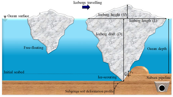
Figure 1. Scheme of the iceberg in free-floating and ice-gouging conditions.

When icebergs collide with offshore structures such as bridges, risers, or pipelines, they can exert significant horizontal and vertical loads, depending on their mass, draft, and drift velocity. These interactions may lead to structural instability, soil deformation, or direct damage. The magnitude and duration of these loads are influenced by keel geometry, seabed contact, and infrastructure embedment. Incorporating these collision scenarios into the modeling framework could further improve infrastructure resilience in ice-prone waters.

Compared to icebergs, other floating objects such as plastic debris or timber exhibit significantly lower mass and draft-to-volume ratios. While they can pose navigational hazards or environmental concerns, their interaction with the seabed or underwater infrastructure is minimal due to their buoyancy and negligible keel penetration. In contrast, icebergs can gouge the seabed and cause substantial subgouge soil deformation, which justifies the development of specialized models for iceberg-specific scenarios.

Effective iceberg management systems and ensuring the operational safety of seabed-anchored structures against iceberg impacts in ice-affected areas require accurate estimation of iceberg depth, which can help reduce operational expenses and service interruptions. Previous research has concentrated on forecasting iceberg depth using measurements such as iceberg size or mass. For instance, researchers including Allaire [5], Robe and Farmer [6], Bass [7], Hotzel and Miller [8], and C-CORE [9] examined various aspects of iceberg geometry through field studies, theoretical analysis, and computational modeling. Furthermore, Barker et al. [10] analyzed iceberg measurements including both the underwater portion (keel) and above-water section (sail). These researchers assessed the cross-sectional areas of icebergs at various underwater depths from specific waterline measurements. They developed mathematical formulas based on length to calculate iceberg depth using regression analysis and power curve techniques. Dowdeswell and Bamber [11] studied the keel depth of drifting icebergs in Antarctic waters, estimating underwater depth based on surface height and area measurements. Their research found that only a limited number of icebergs in Greenland and Antarctic waters had depths exceeding 650 m. Stuckey [12] calculated iceberg drift speed using probabilistic methods, noting that factors such as above-water dimensions, underwater size, and iceberg shape influenced environmental forces. In a separate investigation, McKenna and King [13] forecasted the deterioration patterns of various icebergs by observing cumulative changes in depth, mass, and structural formation. Their analysis emphasized that iceberg depth and length decreased as mass was reduced. King [14] modeled iceberg characteristics including depth, length, and mass using Monte Carlo simulation techniques, concluding that assessment of iceberg depths beyond 150 m was quite limited. Turnbull et al. [15] tracked the drift patterns of temporary icebergs in Northwest Greenland using retrospective simulation, revealing that iceberg trajectories could be influenced by their depth. King et al. [16] conducted field research to measure iceberg rotation rates, calculating depths through a calving methodology with computed standard deviations of depth variations ranging from 19% to 34%. They found correlations between iceberg depths and masses. Turnbull et al. [17] proposed a formula for estimating the drift of traveling icebergs on Canada’s Grand Banks, though this equation overestimated iceberg depths by approximately 1.3 times compared to actual observations. McKenna et al. [18] simulated ice gouging on Canada’s Grand Banks using Monte Carlo simulation, incorporating iceberg depth variations to minimize the scale of depth changes in their modeling. Stuckey et al. [19] created 3D iceberg models using field data, considering mass and depth in relation to iceberg length based on power law principles. Most recently, Azimi et al. [20] identified dimensionless variable groups that influence iceberg depth estimation for the first time. These authors created linear regression (LR) equations using the identified dimensionless groups and identified the most significant parameters, along with optimal LR models. They presented multiple LR-based models for estimating iceberg depths in practical engineering applications, with their best LR model outperforming previous empirical relationships. Over the past thirty years, many researchers have studied the factors affecting sub-gouge soil properties. Scholars such as Paulin [21], Paulin [22], Lach [23], Woodworth-Lynes et al. [24], C-CORE [25,26], Hynes [27], Schoonbeek et al. [28], Been et al. [29], and Yang [30] evaluated the interaction between icebergs and seabed materials for sandy or clay substrates in laboratory settings. Recently, Arnau Almirall [31] conducted experimental studies under normal gravity conditions to measure sub-gouge sand characteristics in both saturated and dry conditions. This researcher investigated how velocity changes, scour patterns, and soil properties affected sub-gouge characteristics. The findings showed that ice-scoured sand movements under normal gravity conditions were less significant than results obtained from centrifuge testing environments. The application of machine learning (ML) is becoming increasingly ubiquitous, extending across fields such as engineering and medicine due to its speed, precision, and cost-effectiveness.

ML algorithms have seen limited application in simulating iceberg–seabed interactions. Kioka et al. [32,33] employed a Neural Network (NN) to model ice gouging in sandy seabeds, validating their approach against mechanical methods and confirming strong correlation. Azimi and Shiri [34] identified key dimensionless groups affecting iceberg–seabed interactions in clay and sand using Buckingham’s theorem, proposing linear regression (LR)-based equations for subgouge soil deformations. Later, they used gene expression programming (GEP) to model horizontal deformations in sand, highlighting the dilation index, gouge depth, and attack angle as critical inputs [35]. Further studies [36,37] applied various NN-based techniques—including ANN, ELM, Sa-ELM, GMDH, and GS-GMDH—to predict subgouge soil behavior in clay and sand. To address NN limitations such as overfitting, data scarcity, and hyperparameter tuning, Azimi et al. [38,39] adopted tree-based algorithms (DTR, RFR, GBR), finding the Extra Trees Regressor (ETR) most effective. Despite these advances, no study has simultaneously modeled iceberg draft and subgouge soil characteristics (reaction forces, deformations) across seabed types. This study bridges that gap by employing the ETR algorithm to predict these parameters in both sandy and clay seabeds, with the following key objectives:

• Establishing an ETR model to simulate the iceberg draft and subgouge soil features simultaneously.
• Analyzing the simulation results to identify the superior ETR models.
• Determination of the most influential input parameters to predict the iceberg draft and subgouge soil characteristics in clay and sandy seabed.

While the methodology represents a significant advancement, the innovation of this research extends well beyond methodological improvements and addresses several critical limitations of our previous studies. Our earlier work modeled iceberg draft, iceberg–seabed interaction in sand seabeds, or iceberg–seabed interaction in clay seabeds as separate, isolated components using different machine learning algorithms.

This integration represents a fundamental shift from fragmented, single-parameter modeling to holistic iceberg behavior simulation. The key innovations include:

(1)

the development of cross-parameter dependencies that capture the complex relationships between draft characteristics and seabed interactions, which were previously ignored in isolated models;

(2)

the implementation of a multi-output prediction system that enables real-time assessment of multiple iceberg parameters simultaneously, significantly improving operational efficiency;

(3)

the creation of seabed-agnostic modeling capabilities that can adapt to varying geological conditions without requiring separate model deployments; and

(4)

enhanced prediction accuracy through synergistic modeling, where draft predictions inform seabed interaction calculations and vice versa.

The framework’s ability to simultaneously consider multiple interaction scenarios represents a significant advancement in predictive capability and operational applicability for offshore operations and infrastructure protection.

More details about the applied methodology and simulation results will be provided in the forthcoming sections.

2. Materials and Methods

Figure 2 illustrates the flowchart outlining this study. In this research, datasets related to iceberg draft and subgouge soil properties were developed and split into training and testing sets. The training data was used to train the ETR algorithm, while the model’s performance was evaluated using the testing data. Through a series of analyses, the most effective ETR models and the key input variables were identified.

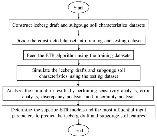
Figure 2. Flowchart of the present research.

2.1. Extra Tree Regression (ETR)

The Extra Trees Regressor (ETR) algorithm represents an advanced iteration of the Random Forest (RF) method introduced by Geurts et al. [40]. While both algorithms employ bootstrap aggregation (bagging) and construct multiple decision trees for regression tasks, ETR introduces two key modifications: (1) random selection of split points during node partitioning, and (2) utilization of the complete training dataset to reduce bias. The ETR approach incorporates two critical parameters—κ (controlling random feature selection) and ռ (governing sample size for node splitting)—which collectively enhance model robustness by mitigating overfitting and improving predictive accuracy [41]. Notably, the current study implemented hyperparameter optimization for ETR through an empirical trial-and-error approach, with detailed configurations provided in Table 1. Key improvements in this version:

Table 1. Results of the hyperparameter tuning of the ETR algorithm in the current research.

Hyperparameter	Value
min_samples_leaf	1
min_samples_split	8
max_features	1
random_state	None
max_depth	None
min_impurity_decrease	0
max_leaf_nodes	None
min_weight_fraction_leaf	0
ccp_alpha	0

• Removed redundancy while preserving technical precision
• Improved flow between concepts
• Maintained all critical technical details (κ, ռ parameters, bias reduction)
• Clarified the relationship between RF and ETR
• Kept all essential citations
• Structured the information more logically

The parameters listed in Table 1 are hyperparameters used to optimize the ETR algorithm’s learning process and tree structure. These are not physical or environmental constants and may be adjusted for different datasets or applications. For consistency, these values were held constant throughout the present study to ensure comparability across models.

2.2. Iceberg Draft

The iceberg draft (D) was considered in terms of the physical features of the iceberg, such as the iceberg length (L), iceberg height (H), iceberg width (W), and iceberg mass (M). Azimi et al. [18] introduced the dimensionless groups governing the iceberg draft in the following form:

$${\displaystyle \frac{D}{H}}=f_6\left({\displaystyle \frac{L}{H}},{\displaystyle \frac{W}{H}},{\displaystyle \frac{M}{{\rho }_i.H^3}},S_f\right)$$

(1)

Hence, the iceberg draft ratio (D/H) is a function of the length ratio (L/H), width ratio (W/H), mass ratio $\left(M/{\rho }_i.H^3\right)$, and iceberg shape factor $\left(S_f\right)$. In the present research, the ETR algorithm was fed with the dimensionless groups in Equation (1) as inputs to simulate the iceberg draft ratio.

The iceberg–seabed interaction parameters (η) in a soil mass such as soil deformations (d/W) and reaction forces (F/γsW³) are a function of several parameters like the scour depth (D_s), the shear strength parameter of the soil (c), the internal friction angle of soil (φ), the width of gouge (W), the attack angle (α), the angle of the surcharged soil slope (ω), the height of the berm (h^′), the horizontal load (L_h), the vertical load (L_v), the velocity of iceberg keel (V), and the specific weight of sand (${\gamma }_s$) [23,34,35]:

$${\eta }_{\left(soil\right)}=f_1\left(D_s,c, \phi ,W,\alpha ,\omega ,h^{\prime },L_h,L_v,V,{\gamma }_s\right)$$

(2)

Equation (2) can be written in the form of Equations (3) and (4) for the sandy and clay seabed as follows [34]:

$${\displaystyle \frac{d_{\left(sand\right)}}{W}},{\displaystyle \frac{F_{\left(sand\right)}}{{\gamma }_s{W}^3}}= f_3\left({\displaystyle \frac{y}{W}},{\displaystyle \frac{D_s}{W}},\phi ,\alpha ,{\displaystyle \frac{h^{\prime }}{W}},{\displaystyle \frac{L_h}{{\gamma }_s{W}^3}},{\displaystyle \frac{L_v}{{\gamma }_s{W}^3}},{\displaystyle \frac{V^2}{gW}}\right)$$

(3)

$${\displaystyle \frac{d_{\left(clay\right)}}{W}}, {\displaystyle \frac{F_{\left(clay\right)}}{{\gamma }_s{W}^3}}=f_3\left({\displaystyle \frac{y}{W}},{\displaystyle \frac{D_s}{W}},{\displaystyle \frac{c}{{\gamma }_s.W}},\alpha ,\omega ,{\displaystyle \frac{h^{\prime }}{W}},{\displaystyle \frac{L_h}{{\gamma }_s{W}^3}},{\displaystyle \frac{L_v}{{\gamma }_s{W}^3}},{\displaystyle \frac{V^2}{gW}}\right)$$

(4)

2.3. Constructed Dataset

To ensure the reliability and accuracy of the machine learning (ML) models developed for iceberg draft modeling, the field measurements described in Section 2.3.1 were utilized for validation purposes. These real-world data points served as a benchmark to assess how well the models could replicate observed iceberg drafts under various conditions. In parallel, to verify the performance of the ML models designed for simulating iceberg–seabed interactions, the experimental data presented in Section 2.3.2 were employed. These experimental values provided a controlled basis for evaluating the models’ ability to reproduce the physical phenomena involved in iceberg-grounding scenarios, thereby strengthening the overall credibility of the simulation outcomes.

2.3.1. Iceberg Draft Dataset

Observational data from multiple field studies on iceberg drafts were compiled into a comprehensive dataset for training and testing the ETR algorithm. Key measurements from 12 documented field investigations [20] were incorporated. Table 2 summarizes these field studies used to build the iceberg draft dataset. For modeling purposes with the ETR algorithm, 60% of the dataset was used for training, while the remaining 40% was reserved for testing.

Table 2. Summary of the applied field works in the present research to construct the iceberg draft dataset.

Research	Number of Case Studies
El-Tahan et al. [42]	38 cases
Woodworth-Lynas et al. [43]	One case
Løset and Carstens [44]	52 cases
Barker et al. [8]	14 cases
McKenna [45]	Two cases
Sonnichsen et al. [46]	Nine cases
Turnbull et al. [13]	Two cases
McGuire et al. [47]	Eight cases
Younan et al. [48]	29 cases
Talimi et al. [49]	One case
Zhou [50]	Three cases
Turnbull et al. [15]	Two cases

2.3.2. Iceberg–Seabed Interaction

The experimental values of six laboratory studies recorded by Paulin [21,22] (P-1 to P-5), C-CORE [25] (C’-1 to C’-10), Hynes [27] (H-1 to H-5), and Yang [30] (Y-1 to Y-7) were employed to verify the ETR algorithm. The amount of the surcharged soil slope (ω) was not mentioned in the previous works. The internal friction angle of sand (φ), the keel attack angle (α), the gouge depth ratio (Ds/W), and the velocity ratio (V²/gW) in Paulin’s [21] study (P-1) were reported at 18°, 15°, 0.093, and 0.00054, in turn. However, the berm height ratio (h^′/W) was not provided in the P-1 case.

A set of laboratory studies were also applied in the estimation of the iceberg–seabed interaction mechanism in clay seabed. This means that the key parameters of five laboratory works documented by C-CORE [25,26] (C-1 to C-12), Lach [23] (L-1 to L-8), Schoonbeek et al. [28] (S-1), and Been et al. [29] (B-1 to B-5) were adopted to validate the ETR algorithm. To simulate the subgouge soil parameters, 70% of the built dataset was for the training of the ETR models, and 30% of the rest data was considered in the testing mode. The applied input combinations to develop different ETR models in this work are depicted in Figure 3. It is worth mentioning that the results from the testing phase were analyzed in the present research.

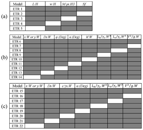
Figure 3. Input combinations for development of ETR models (a) iceberg draft (b) iceberg–seabed interaction in the sand (c) iceberg–seabed interaction in clay.

Cross-validation was not implemented in this study; however, the robustness of the ETR models was evaluated through multiple training-testing configurations to ensure the reliability of the results. Different ratios of dataset splits ranging from 50–50% to 80–20% were systematically employed to train and test the machine learning models, with data selection performed randomly for each configuration. This approach was adopted to rest assure that the presented results were not dependent on a single data partition and to verify the consistency of model performance across various training-testing scenarios. The multiple ratio testing demonstrated that the ETR model maintained consistent performance metrics across different data splits, thereby confirming that the reported accuracy levels were not random in nature but represented genuine predictive capability of the modeling framework.

2.4. Goodness of Fitness

To evaluate the accuracy, correlation strength, and complexity of the ETR models, various statistical metrics were utilized, including the correlation coefficient (R), root mean square error (RMSE), mean absolute percentage error (MAPE), Willmott Index (WI), coefficient of residual mass (CRM), and Akaike Information Criterion (AIC). High values of R and WI, approaching one, indicated strong agreement between the ETR model and observed data. Conversely, lower values of RMSE, MAPE, and CRM signified minimal error and greater precision in the model’s predictions. Since the aforementioned indices did not account for model complexity, AIC was introduced to address this aspect. A lower AIC value reflected a simpler and more efficient model. Therefore, the optimal ETR model would combine minimal error (RMSE, MAPE, CRM) and complexity (AIC) with maximum correlation (R and WI) [36,37]:

$$R={\displaystyle \frac{{\sum }_{i=1}^n\left(P_i-\overline{P}\right)\left(O_i-\overline{O}\right)}{\sqrt{{{\sum }_{i=1}^n\left(P_i-\overline{P}\right)}^2}{{\sum }_{i=1}^n\left(O_i-\overline{O}\right)}^2}}$$

(5)

$$RMSE=\sqrt{{\displaystyle \frac{1}{n}}{{\sum }_{i=1}^n\left(P_i-O_i\right)}^2}$$

(6)

$$MAPE={\displaystyle \frac{100}{n}}{\sum }_{i=1}^n\left|{\displaystyle \frac{P_i-O_i}{O_i}}\right|$$

(7)

$$WI=1-{\displaystyle \frac{{\sum }_{i=1}^n{\left(O_i-P_i\right)}^2}{{\sum }_{i=1}^n{\left(\left|P_i-\overline{O}\right|+\left|O_i-\overline{O}\right|\right)}^2}}$$

(8)

$$CRM={\displaystyle \frac{{\sum }_{i=1}^n{O}_i-{\sum }_{i=1}^n{P}_i}{{\sum }_{i=1}^n{O}_i}}$$

(9)

$$AIC=n\times \mathit{log}\left(\sqrt{{\displaystyle \frac{1}{n}}{{\sum }_{i=1}^n\left(P_i-O_i\right)}^2}\right)+2k$$

(10)

Here, O_i, P_i, $\overline{O}$, $\overline{P}$, n, and k are the observational value, the simulated amount, the average field or experimental measurements, the average simulated amount, the number of observations, and the number of independent variables in the ETR models.

The selected statistical indicators (R, RMSE, MAPE, WI, CRM, AIC) were chosen based on their widespread application in regression and machine learning studies for evaluating model accuracy, consistency, and complexity. For example, RMSE and MAPE quantify prediction error magnitude, while WI and CRM reflect agreement with observed trends. AIC additionally accounts for model parsimony. Similar performance metrics were adopted in iceberg–seabed interaction modeling by Kioka et al. [32,33] and Azimi et al. [38,39].

3. Results and Discussion

The performance of the ETR models is assessed using a range of analyses, such as sensitivity analysis, error evaluation, and uncertainty assessment. Following this, the most effective ETR models for predicting iceberg drafts and subgouge soil characteristics, along with the most impactful input variables, are identified. Further analyses are then conducted on these top-performing models.

3.1. Sensitivity Analysis

The key statistical indices obtained from the developed ETR models are arranged in Table 3. Among the ETR models in the iceberg draft estimation, the ETR 1 model as a function of all inputs comprising $L/H,W/H, M/{\rho }_i.H^3, \mathrm{a}\mathrm{n}\mathrm{d} S_f$ was known as the model with the highest degree of accuracy, signifying that the RMSE value was achieved as 1.081. The effect of the iceberg shape factor was ignored in ETR 2, where the lowest value of CRM was computed for this model (CRM = 0.087). To predict the iceberg draft using the ETR 3, the mass ratio ($M/{\rho }_i.H^3$) was an eliminated input and the value of AIC for this model was 8.888. The correlation coefficient (R) and Willmott Index (WI) criteria for the ETR 4 were estimated as 0.923 and 0.926, where the influence of the iceberg width ratio ($W/H$) was omitted. The ETR 5 model showed the worst performance in approximating the iceberg draft as the impact of $L/H$ was removed from the ETR 5 model’s inputs, with the RMSE, R, and AIC indices of 1.234, 0.887, and 11.837.

Table 3. Key statistical indices calculated for the ETR models.

Parameter	Model	R	RMSE	AIC	CRM	WI
Draft	ETR 1	0.920	1.081	10.165	0.101	0.943
	ETR 2	0.906	1.150	9.882	0.087	0.933
	ETR 3	0.917	1.109	8.888	0.108	0.940
	ETR 4	0.923	1.161	10.138	0.107	0.926
	ETR 5	0.887	1.234	11.837	0.102	0.926
Sand-Horizontal reaction force	ETR 6	0.985	154,280.556	379.182	−0.030	0.992
	ETR 7	0.983	167,992.998	379.770	−0.035	0.991
	ETR 8	0.982	168,842.614	379.924	−0.033	0.991
	ETR 9	0.983	165,178.002	379.257	−0.035	0.991
	ETR 10	0.994	99,805.670	363.941	0.004	0.997
	ETR 11	0.982	171,349.321	380.372	−0.040	0.991
	ETR 12	0.982	169,286.105	380.003	−0.038	0.991
	ETR 13	0.986	150,379.199	376.403	−0.033	0.993
	ETR 14	0.880	439,271.280	408.991	−0.058	0.938
Sand-Vertical reaction force	ETR 6	0.970	46.348	107.632	−0.059	0.983
	ETR 7	0.973	44.818	104.830	−0.066	0.984
	ETR 8	0.974	43.953	104.364	−0.079	0.985
	ETR 9	0.972	45.123	104.992	−0.059	0.984
	ETR 10	0.973	44.460	104.638	−0.065	0.984
	ETR 11	0.972	45.189	105.027	−0.062	0.984
	ETR 12	0.972	44.911	104.880	−0.064	0.984
	ETR 13	0.972	45.027	104.941	−0.061	0.984
	ETR 14	0.926	70.017	115.486	−0.044	0.959
Sand-Horizontal deformation	ETR 6	0.739	0.187	−18.256	−0.094	0.849
	ETR 7	0.980	0.073	−39.551	0.180	0.974
	ETR 8	0.984	0.072	−39.618	0.193	0.973
	ETR 9	0.982	0.079	−37.901	0.197	0.968
	ETR 10	0.981	0.079	−37.872	0.211	0.968
	ETR 11	0.981	0.078	−38.078	0.199	0.968
	ETR 12	0.982	0.074	−39.172	0.204	0.972
	ETR 13	0.981	0.074	−39.015	0.179	0.972
	ETR 14	0.278	0.245	−14.719	0.416	0.307
Sand-Vertical deformation	ETR 6	0.828	0.009	−28.827	−0.001	0.913
	ETR 7	0.826	0.009	−30.733	−0.012	0.912
	ETR 8	0.818	0.009	−30.560	0.147	0.879
	ETR 9	0.905	0.011	−29.462	−0.227	0.916
	ETR 10	0.818	0.011	−29.495	−0.313	0.849
	ETR 11	0.828	0.010	−30.027	−0.230	0.897
	ETR 12	0.828	0.009	−30.699	−0.089	0.911
	ETR 13	0.828	0.009	−30.776	0.056	0.912
	ETR 14	0.277	0.016	−25.467	0.329	0.207
Clay-Horizontal reaction force	ETR 15	0.988	57,795.569	656.856	0.011	0.994
	ETR 16	0.988	57,521.716	656.577	0.004	0.994
	ETR 17	0.988	56,914.968	655.956	0.006	0.994
	ETR 18	0.989	54,630.154	653.553	−0.003	0.995
	ETR 19	0.988	58,744.465	657.811	0.011	0.994
	ETR 20	0.988	56,624.436	655.656	0.012	0.994
	ETR 21	0.989	55,408.261	654.383	0.010	0.994
	ETR 22	0.794	227,462.840	737.183	−0.020	0.899
Clay-Vertical reaction force	ETR 15	0.995	475.567	225.500	−0.005	0.997
	ETR 16	0.996	478.300	225.696	−0.005	0.997
	ETR 17	0.996	478.067	225.680	−0.004	0.997
	ETR 18	0.996	473.733	225.367	−0.006	0.997
	ETR 19	0.996	476.092	225.538	−0.008	0.997
	ETR 20	0.996	472.658	225.289	−0.006	0.997
	ETR 21	0.996	473.307	225.336	−0.006	0.997
	ETR 22	0.951	1512.420	265.194	0.002	0.959
Clay-Horizontal deformation	ETR 15	0.999	0.091	−36.939	0.007	0.999
	ETR 16	0.999	0.043	−53.137	−0.032	0.999
	ETR 17	0.999	0.046	−51.624	−0.043	0.999
	ETR 18	0.999	0.066	−43.745	−0.057	0.999
	ETR 19	0.999	0.038	−55.679	−0.027	0.999
	ETR 20	0.999	0.037	−56.264	−0.036	0.999
	ETR 21	0.999	0.057	−46.891	−0.045	0.999
	ETR 22	0.999	0.529	0.463	0.221	0.973
Clay-Vertical deformation	ETR 15	0.963	0.012	−53.633	0.098	0.962
	ETR 16	0.983	0.009	−57.192	0.035	0.977
	ETR 17	0.974	0.011	−54.854	0.122	0.968
	ETR 18	0.971	0.011	−54.597	0.118	0.967
	ETR 19	0.920	0.015	−49.616	0.137	0.933
	ETR 20	0.980	0.010	−56.382	0.073	0.974
	ETR 21	0.936	0.014	−51.091	0.138	0.946
	ETR 22	0.432	0.033	−37.753	−0.417	0.521

According to the conducted sensitivity analysis, the iceberg length ratio ($L/H$) was distinguished as the most influencing input to model the iceberg draft utilizing the ETR method; whereas, the iceberg width ratio ($W/H$), the iceberg mass ratio ($M/{\rho }_i.H^3$), and iceberg shape factor ($S_f$) were ranked as the second-effective to the fourth-important inputs.

The ETR 6 to ETR 14 models were defined to approximate the subgouge soil features in the sandy seabed. Among the ETR models in the estimation of the horizontal reaction force, the ETR 10 possessed the highest degree of precision, correlation, and simplicity, signifying that the RMSE, R, and AIC values for this model were appraised to be 99,805.670, 0.994, and 363.941, respectively. The ETR 10 modeled the horizontal reaction forces utilizing $x/W, D_s/W, \phi , \alpha , L_h/{\gamma }_s{W}^3, L_v/{\gamma }_s{W}^3, V^2/gW$, while the influence of $h^{\prime }/W$ was removed from this model. The performed sensitivity analysis proved that the position of the iceberg along the scour axis (x/W), the attack angle (α), and the shear strength parameter of the sand seabed (φ) were recognized to be the most significant inputs.

The ETR 8 model showed up to be the best ETR model in the estimation of the vertical reaction forces in the sandy seabed when the AIC and WI values for such model were obtained as 104.364 and 0.985. The ETR 8 model simulated the vertical reaction forces regarding $x/W, D_s/W, \phi , \alpha , h^{\prime }/W, L_h/{\gamma }_s{W}^3, V^2/gW$ inputs and the $L_v/{\gamma }_s{W}^3$ was dropped from the model’s inputs. Additionally, the $x/W, \alpha$, and $L_h/{\gamma }_s{W}^3$ were detected to be the most effective input parameters to predict the vertical reaction forces.

In ETR 8, the soil depth ratio (y/W) was the most influential input for predicting horizontal deformation in sand. Theoretically, this is consistent with geotechnical principles where deeper soil layers offer greater confinement, affecting shear resistance and deformation propagation. Similar findings were reported in physical modeling studies by Paulin [19] and Hynes [25].

The value of RMSE and AIC for the best ETR model to predict the subgouge horizontal deformation in the sand, the ETR 8 model, was equal to 0.079 and −39.618. These horizontal deformations approximated in terms of $y/W, D_s/W, \phi , \alpha , h^{\prime }/W, L_h/{\gamma }_s{W}^3, V^2/gW$ using the ETR 8 model, where the influence of $L_v/{\gamma }_s{W}^3$ was taken away from the input combinations. The soil depth ratio (y/W) was known as the most important input to simulate the horizontal deformations in the sand, whilst $h^{\prime }/W, L_h/{\gamma }_s{W}^3, \alpha$, $D_s/W, \phi , V^2/gW, \mathrm{a}\mathrm{n}\mathrm{d} L_v/{\gamma }_s{W}^3$ were identified in the second-significant to eighth-significant inputs in terms of effectiveness.

The ETR 9 model surmised the vertical deformation in sand using $y/W, D_s/W, \phi , \alpha , h^{\prime }/W, L_v/{\gamma }_s{W}^3, V^2/gW$ inputs and the impact of $L_h/{\gamma }_s{W}^3$ was disregarded for this model, with the R and WI indices of 0.905 and 0.916. The soil depth ratio (y/W) and the berm height ratio (h^’/W) were the most important input parameters in the vertical deformation estimation in the sand.

In order to estimate the horizontal reaction forces in clay seabed, the ETR 18 model as a function of $x/W, D_s/W, c/{\gamma }_{s}W, \alpha , L_v/{\gamma }_s{W}^3, V^2/gW$ had the best performance, with WI and AIC values of 0.995 and 653.553. The effectiveness of the iceberg along the scour axis (x/W), attack angle (α), and the iceberg dynamic factor (V²/g.W) was much higher than other input parameters to model the horizontal forces in clay. In addition, $L_v/{\gamma }_s{W}^3, c/{\gamma }_{s}W, D_s/W, L_h/{\gamma }_s{W}^3$ were placed in terms of significance in the fourth to seventh positions.

The AIC and RMSE criteria for ETR 20, as the superior model for the vertical reaction force simulation in clay, were surmised as 225.289 and 472.658. The ETR 20 model was inputted with $x/W, D_s/W, \alpha , L_h/{\gamma }_s{W}^3, L_v/{\gamma }_s{W}^3, V^2/gW$ parameters but the clay shear strength parameter ($c/{\gamma }_s.W$) was a removed input in this model. Based on the presented sensitivity analysis, x/W, $D_s/W$, and $L_h/{\gamma }_s{W}^3$ possessed the highest degree of effectiveness and other inputs including $\alpha$, $L_v/{\gamma }_s{W}^3$, $V^2/gW$, and $c/{\gamma }_{s}W$ were ranked in the fourth to seventh places, respectively.

The ETR 20 model was the premium model for the estimation of the horizontal displacements in the clay seabed, with the WI and AIC value of 0.999 and −56.264. The $y/W$, $L_h/{\gamma }_s{W}^3$, $D_s/W$, $L_v/{\gamma }_s{W}^3$, $V^2/gW$, $\alpha$, and $c/{\gamma }_{s}W$ were identified as the most important to the less important inputs to forecast the horizontal deformations in clay.

ETR 16 was the excellent model for the simulation of vertical subgouge deformations in clay seabed, with the highest level of correlation, precision, and lowest degree of complexity (R = 0.983, RMSE = 0.009, AIC = −57.192). The ETR 16 model was fed with $y/W, D_s/W, c/{\gamma }_{s}W, \alpha , L_h/{\gamma }_s{W}^3, \mathrm{a}\mathrm{n}\mathrm{d} L_v/{\gamma }_s{W}^3$ inputs to approximate the vertical deformations and the iceberg dynamic factor (V²/g.W) was an eliminated factor. The sensitivity analysis exhibited that the soil depth ratio (y/W), the keel attack angle ($\alpha$), and the gouge depth ratio (D_s/W) were the most remarkable input parameters in the prediction of clay vertical deformations.

Figure 4 presents the accuracy assessment findings for the ETR models used to predict iceberg depths and sub-gouge soil properties. Around one-third of the iceberg depth predictions generated by the ETR 1 model showed errors below 8%, while the ETR 2, ETR 3, ETR 4, and ETR 5 models achieved this accuracy level for approximately 26%, 32%, 21%, and 29% of their predictions, respectively. For sandy seafloor conditions, nearly half of the horizontal force predictions from the ETR 10 model demonstrated errors under 12%, while roughly 70% of the vertical force predictions from the ETR 8 model showed errors below 16%. Additionally, about one-quarter of the horizontal displacement predictions and one-third of the vertical displacement predictions in sandy substrates, calculated by the ETR 8 and ETR 9 models, respectively, exhibited errors less than 12%. Regarding clay seafloor conditions, approximately 85% of the horizontal force calculations produced by the ETR 18 model contained errors under 18%, while the ETR 20 model achieved errors below this threshold for about 95% of its vertical force predictions. Nearly 45% of the horizontal displacement estimates and 37% of the vertical displacement estimates generated by the ETR 20 and ETR 16 models, respectively, showed errors smaller than 20%.

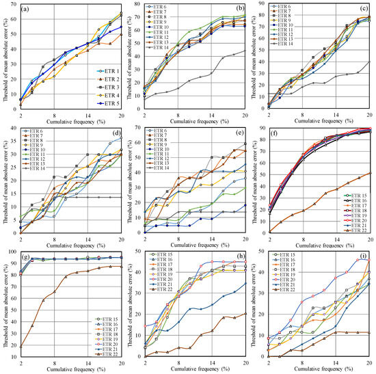
Figure 4. Results of error analysis for the ETR models to simulate (a) iceberg draft (b) horizontal reaction force in the sand (c) vertical reaction force in the sand (d) horizontal deformation in the sand (e) vertical deformation in the sand (f) horizontal reaction force in clay (g) vertical reaction force in clay (h) horizontal deformation in clay (i) vertical deformation in clay.

3.2. Uncertainty Analysis

The study performed an uncertainty analysis (UA) to further evaluation of the ETR models’ performance. In other words, the ETR model’s error $\left(e_j\right)$ were computed as the difference between the predicted value $\left(P_j\right)$ through this model and the observed value $\left(O_j\right),$ as follows:

$$e_j=P_j-O_j$$

(11)

The mean $\left(Mean\right)$ and the standard deviation $\left(StDev\right)$ of such error values were calculated by the equations below:

$$\mathrm{M}\mathrm{e}\mathrm{a}\mathrm{n}={\displaystyle \frac{1}{n}}{\sum }_{j=1}^n{e}_j$$

(12)

$$\mathrm{S}\mathrm{t}\mathrm{D}\mathrm{e}\mathrm{v}=\sqrt{{\sum }_{j=1}^n{\left(e_j-\overline{e}\right)}^2/\left(n-1\right)}$$

(13)

When an individual ETR model produced a negative Mean value, it indicated that the model underestimated the sub-gouge soil parameters or iceberg depth; conversely, a positive Mean value signified that the ETR model overestimated the target parameter. Therefore, a confidence interval (CI) was calculated around the computed error using the Mean and standard deviation (StDev) values, along with the “Wilson score method” while excluding the continuity correction. The Wilson score interval, which is a normal distribution interval modified as an asymmetric normal distribution, was utilized to determine the CI boundaries. Subsequently, applying ±1.96 Se resulted in a 95% confidence interval. It is important to note that the width of the uncertainty bound (WUB) for each ETR model was obtained as shown below [36]:

$$WUB=\pm {\displaystyle \frac{\left(Lower bound-upper bound\right)}{2}}$$

(14)

Table 4 presents the outcomes of the uncertainty analysis conducted for the ETR models. The analysis showed that all models developed to simulate iceberg drafts (ETR 1 to ETR 5) tended to overestimate, with ETR 1 exhibiting the tightest uncertainty range (WUB = ±0.254). Similarly, models ETR 6 to ETR 14 overestimated horizontal reaction forces in sandy seabeds, with ETR 10 demonstrating the narrowest WUB and standing out as the most accurate. For vertical reaction forces in sandy seabeds, the top-performing model showed an underestimation, with a Mean of −2.060 and WUB of ±8.700. Horizontal deformations in sandy seabeds were also overestimated by models ETR 6 to ETR 14. In clay seabeds, ETR 18 yielded the lowest Mean and tightest WUB for horizontal reaction forces, though it still overestimated the values. Conversely, ETR 20, the best model for vertical reaction forces in clay, underestimated the target. Overall, the uncertainty analysis indicated that ETR 20 and ETR 16—identified as the leading models—were biased toward underestimating and overestimating horizontal and vertical subgouge deformations in clay seabeds, respectively. The uncertainty analysis showed that the WUB for vertical reaction force predictions in sand (ETR 8) was ±8.7, while that for iceberg draft (ETR 1) was ±0.254. These relatively narrow intervals support the reliability of the ETR predictions.

Table 4. Results of uncertainty analysis for the ETR models.

Parameter	Model	Mean	StDev	95%CI		WUB
Draft	ETR 1	0.39	1.016	0.136	0.644	±0.254
	ETR 2	0.335	1.109	0.059	0.612	±0.277
	ETR 3	0.415	1.037	0.156	0.674	±0.259
	ETR 4	0.411	1.094	0.137	0.684	±0.274
	ETR 5	0.395	1.178	0.1	0.689	±0.295
Sand-Horizontal reaction force	ETR 6	7010.948	94,635.970	−16,823	30,845	±23,834
	ETR 7	6948.011	98,479.210	−17,854	31,750	±24,802
	ETR 8	8940.125	92,871.530	−14,449	32,330	±23,389.500
	ETR 9	7094.299	95,202.510	−16,882	31,071	±23,976.500
	ETR 10	12,830.91	85,894.21	−8801	34,436	±21,618.500
	ETR 11	5328.068	97,348.02	−19,189	29,845	±24,517
	ETR 12	6038.568	97,902.03	−18,618	30,695	±24,656.500
	ETR 13	4120.492	98,780.39	−20,757	28,998	±24,877.500
	ETR 14	38,833.970	238,386.700	−21,203	98,871	±60,037
Sand-Vertical reaction force	ETR 6	0.453	33.726	−8.940	9.840	±9.390
	ETR 7	−0.586	32.718	−9.690	8.520	±9.105
	ETR 8	−2.060	31.235	−10.760	6.640	±8.700
	ETR 9	0.195	32.835	−8.950	9.340	±9.145
	ETR 10	−0.472	32.171	−9.430	8.480	±8.955
	ETR 11	−0.167	32.783	−9.290	8.960	±9.125
	ETR 12	−0.278	32.495	−9.330	8.770	±9.050
	ETR 13	0.087	32.607	−8.990	9.160	±9.075
	ETR 14	5.049	56.605	−10.710	20.810	±15.760
Sand-Horizontal deformation	ETR 6	0.019	0.084	−0.007	0.045	±0.026
	ETR 7	0.016	0.074	−0.007	0.040	±0.024
	ETR 8	0.018	0.074	−0.006	0.041	±0.024
	ETR 9	0.018	0.081	−0.007	0.043	±0.025
	ETR 10	0.019	0.081	−0.006	0.045	±0.026
	ETR 11	0.018	0.080	−0.007	0.043	±0.025
	ETR 12	0.018	0.075	−0.005	0.042	±0.024
	ETR 13	0.016	0.077	−0.008	0.040	±0.024
	ETR 14	0.038	0.258	−0.042	0.119	±0.081
Sand-vertical deformation	ETR 6	0.001	0.008	−0.002	0.005	±0.004
	ETR 7	0.001	0.008	−0.003	0.005	±0.004
	ETR 8	0.003	0.008	−0.0003	0.007	±0.004
	ETR 9	−0.004	0.010	−0.009	0.0007	±0.005
	ETR 10	−0.004	0.008	−0.008	−0.0006	±0.004
	ETR 11	−0.003	0.008	−0.006	0.0008	±0.003
	ETR 12	−0.0003	0.008	−0.004	0.003	±0.004
	ETR 13	0.002	0.008	−0.001	0.006	±0.004
	ETR 14	0.006	0.015	−0.001	0.013	±0.007
Clay-Horizontal reaction force	ETR 15	6936.124	53,473.540	−2271	16,143	±9207
	ETR 16	4131.597	53,311.010	−5048	13,311	±9179.500
	ETR 17	4786.232	52,530.400	−4259	13,831	±9045
	ETR 18	1655.058	50,082.490	−6968	10,278	±8623
	ETR 19	6782.686	54,190.590	−2548	16,113	±9330.500
	ETR 20	7050.163	52,443.450	−1980	16,080	±9030
	ETR 21	6556.398	50,604.960	−2157	15,270	±8713.500
	ETR 22	8330.371	202,623.600	−26,558	43,219	±34,888.500
Clay-Vertical reaction force	ETR 15	−71.925	473.101	−177.900	34	±105.950
	ETR 16	−66.530	476.6775	−173.300	42.200	±107.750
	ETR 17	−55.842	477.829	−162.900	51.200	±107.050
	ETR 18	−78.119	470.233	−183.400	27.200	±105.300
	ETR 19	−106.604	466.960	−211.200	−2	±104.600
	ETR 20	−86.388	467.666	−191.100	18.400	±104.750
	ETR 21	−80.068	469.467	−185.200	25.100	±105.150
	ETR 22	35.192	1521.672	−306	376	±341
Clay-Horizontal deformation	ETR 15	0.007	0.098	−0.023	0.038	±0.031
	ETR 16	−0.007	0.040	−0.019	0.006	±0.012
	ETR 17	−0.012	0.045	−0.026	0.002	±0.014
	ETR 18	−0.017	0.068	−0.039	0.004	±0.022
	ETR 19	−0.006	0.037	−0.017	0.005	±0.011
	ETR 20	−0.009	0.034	−0.019	0.002	±0.011
	ETR 21	−0.011	0.056	−0.028	0.006	±0.017
	ETR 22	0.092	0.570	−0.085	0.270	±0.177
Clay-Vertical deformation	ETR 15	0.003	0.012	−0.001	0.007	±0.004
	ETR 16	0.001	0.009	−0.002	0.004	±0.003
	ETR 17	0.003	0.010	−0.0003	0.007	±0.004
	ETR 18	0.003	0.011	−0.0005	0.007	±0.004
	ETR 19	0.004	0.015	−0.001	0.009	±0.005
	ETR 20	0.002	0.010	−0.001	0.006	±0.004
	ETR 21	0.004	0.013	−0.0009	0.008	±0.004
	ETR 22	−0.011	0.032	−0.022	−0.0003	±0.011

3.3. Superior ETR Models

The analysis revealed that models ETR 1, ETR 10, ETR 8, ETR 8, ETR 9, ETR 18, ETR 20, ETR 20, and ETR 16 were the most effective for simulating, respectively, the iceberg draft, horizontal reaction forces in clay, vertical reaction forces in clay, horizontal deformations in clay, vertical deformations in clay, horizontal reaction forces in sand, vertical reaction forces in sand, horizontal deformations in sand, and vertical deformations in sand. To evaluate the accuracy of these top-performing models, a discrepancy analysis was carried out. The outcomes of this analysis for the ETR models are illustrated in Figure 5. Model efficiency was assessed using the discrepancy ratio (DR) defined as follows:

$$DR={\displaystyle \frac{P_i}{O_i}}$$

(15)

where $P_i$ and $O_i$ are the predicted and observed values. The closer the magnitude of DR is to unity, the higher performance shows the ETR model. The value of the maximum (DR_(max)), minimum (DR_(min)), and average (DR_(ave)) discrepancy ratio for these models was computed. For instance, the DR_(max), DR_(min), and DR_(ave) values for the ETR 1 model equaled 1.778, 0.493, and 0.960. Moreover, the DR_(ave) criterion for the subgouge soil features in sandy seabed predicted by the ETR 10, ETR 8, ETR 8, and ETR 9 models was acquired to be 1.273, 0.897, 1.463, and 1.206, respectively, and this index for ETR 18, ETR 20, ETR 20, and ETR 16 models to estimate the subgouge soil parameters in clay seabed was at 1.062, 1.078, 1.455, and 1.458.

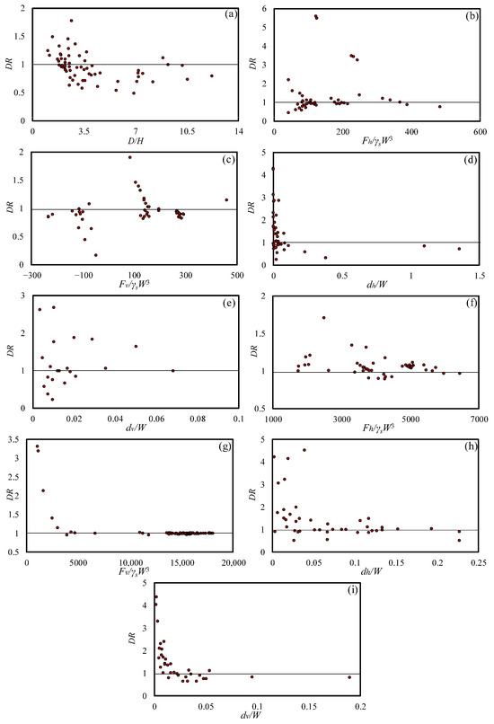
Figure 5. Results of discrepancy analysis for the simulation of (a) iceberg draft by ETR 1 (b) horizontal reaction force in the sand by ETR 10 (c) vertical reaction force in the sand by ETR 8 (d) horizontal deformation in sand by ETR 8 (e) vertical deformation in sand by ETR 9 (f) horizontal reaction force in clay by ETR 18 (g) vertical reaction force in clay by ETR 20 (h) horizontal deformation in clay by ETR 20 (i) vertical deformation in clay by ETR 16.

Discrepancy ratios for the best-performing models (e.g., DR_(ave) = 0.960 for ETR 1, DR_(ave) = 1.078 for ETR 20) indicate close agreement between predictions and observations. These values support the model’s capacity to generalize well across test cases, further reinforcing the quantitative value of the selected ETR models.

ETR 10 emerged as the most effective model for estimating horizontal reaction forces in the sandy seabed. Figure 6 illustrates a comparison between ETR 10′s predictions and the experimental data. The lowest horizontal reaction force was observed at the onset of the scouring process, gradually increasing along the scour path. Although the lab measurements (C’-2, C’-4, and H-2) displayed some fluctuations, ETR 10 demonstrated strong performance in capturing this behavior. In contrast, ETR 4 tended to overestimate the horizontal reaction forces, following a nonlinear trend as seen in cases like C’-3, C’-5, and H-4.

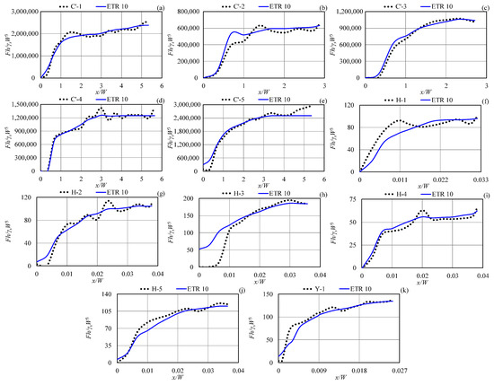
Figure 6. Horizontal reaction force profiles in sandy seabed simulated by ETR 10 (a–e) C’-1 to C’-5 (f–j) H-1 to H-5 (k) Y-1.

Figure 7 presents a comparison between the vertical reaction forces predicted by ETR 8 and those obtained from laboratory experiments. The simulation indicated that these forces were nearly zero at the onset of the ice gouging process and gradually increased along the scour path. Although the experimental data exhibited noticeable fluctuations, ETR 8 was able to capture the vertical reaction forces using a nonlinear approach with satisfactory accuracy.

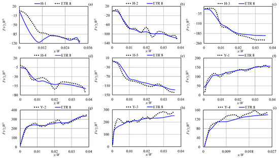
Figure 7. Vertical reaction force profiles in sandy seabed simulated by ETR 8 (a–e) H-1 to H-5 (f–i) Y-1 to H-4.

Figure 8 illustrates the horizontal deformation patterns in a sandy seabed, as modeled by ETR 8. The highest deformation occurred directly below the iceberg keel and diminished with increasing soil depth. The ETR 8 simulation represented these deformations as an exponential curve beneath the iceberg’s contact area, with seabed shear resistance causing the sand deformation to extend deeper than the iceberg’s tip (as seen in points P-1 to P-5, H-3, and Y-1). In contrast, the ML model produced an overestimation of the target parameter, displaying nonlinear trends (evident in points C’-5, H-5, and Y-1).

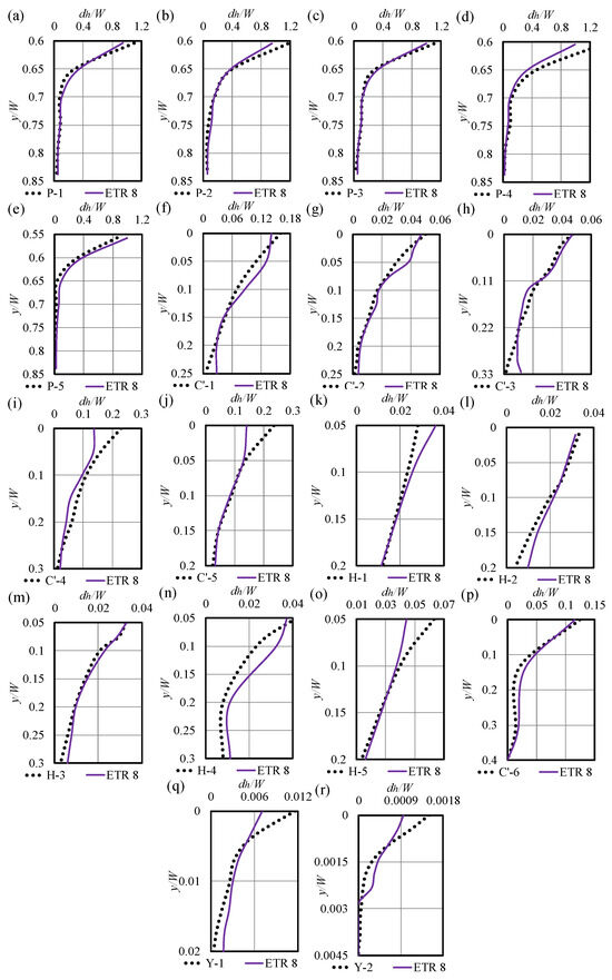
Figure 8. Horizontal deformation profiles in sandy seabed simulated by ETR 8 (a–e) P-1 to P-5 (f–j) C’-1 to C’-5 (k–o) H-1 to H-5 (p) C’-6 (q,r) Y-1 to Y 2.

Figure 9 shows the vertical deformation patterns in the sandy seafloor as predicted by the ETR 9 model. This machine learning model captured vertical deformation using both straight-line (H-2) and curved (P-1, P-3, C’-1, and C’-2) trends, despite numerous variations observed in the experimental data (P-2, P-3, and H-1). Some discrepancies were noted between the actual measurements and the model predictions (P-1, P-2, P-4, C’-1, and C’-2); however, the ETR 9 model attempted to simulate the vertical deformations as accurately as possible.

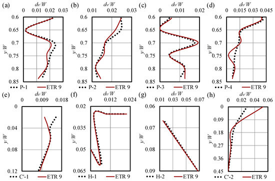
Figure 9. Vertical deformation profiles in sandy seabed simulated by ETR 9 (a–d) P-1 to P-4 (e) C’-1 (f,g) H-1 to H-2 (h) C’-2.

Figure 10 illustrates a comparison between the horizontal reaction forces in a clay seabed predicted by ETR 18 and those measured in laboratory experiments. As with the sandy seabed, the lowest horizontal reaction force was observed at the initial point of the scouring process (x = 0.0), with values increasing along the scour path. Despite some fluctuations in the experimental data (L-1, L-2, and L-7), ETR 18 demonstrated exceptional accuracy, strong correlation, and model simplicity in simulating these forces, particularly evident in cases like C-5 and L-4.

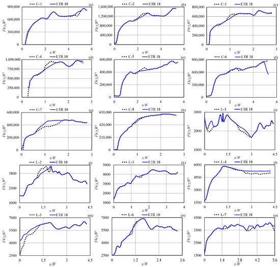
Figure 10. Horizontal reaction force profiles in clay seabed simulated by ETR 18 (a–h) C-1 to C-8 (i–o) L-1 to L-7.

Figure 11 compares the vertical reaction force profiles in the clay seabed simulated by ETR 20 with experimental measurements. The minimum vertical reaction force occurred at the initial point of the scouring process, increasing to its maximum value along the scouring axis. The ETR 20 model underestimated the objective function following a nonlinear trend (L-3 and L-4). Despite variations noted in the laboratory data, the model aimed to approximate the vertical reaction forces as accurately as possible.

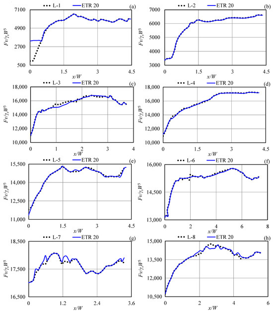
Figure 11. Vertical force profiles in clay seabed simulated by ETR 20 (a–h) L-1 to L-8.

Figure 12 shows a comparison between experimental results and the horizontal deformation in clay seafloor as predicted by the ETR 20 model. The findings indicated that the greatest horizontal deformations occurred at the contact zone between the clay seabed and the iceberg’s base, with deformation decreasing at deeper soil levels. The ETR 20 model exhibited outstanding accuracy in predicting horizontal displacements (C-1, C-2, C-3, C-7, L-4, L-5, and L-7), while only minor discrepancies were observed during the modeling process (C-4, L-2, C-9, C-10, C-11, and C-12).

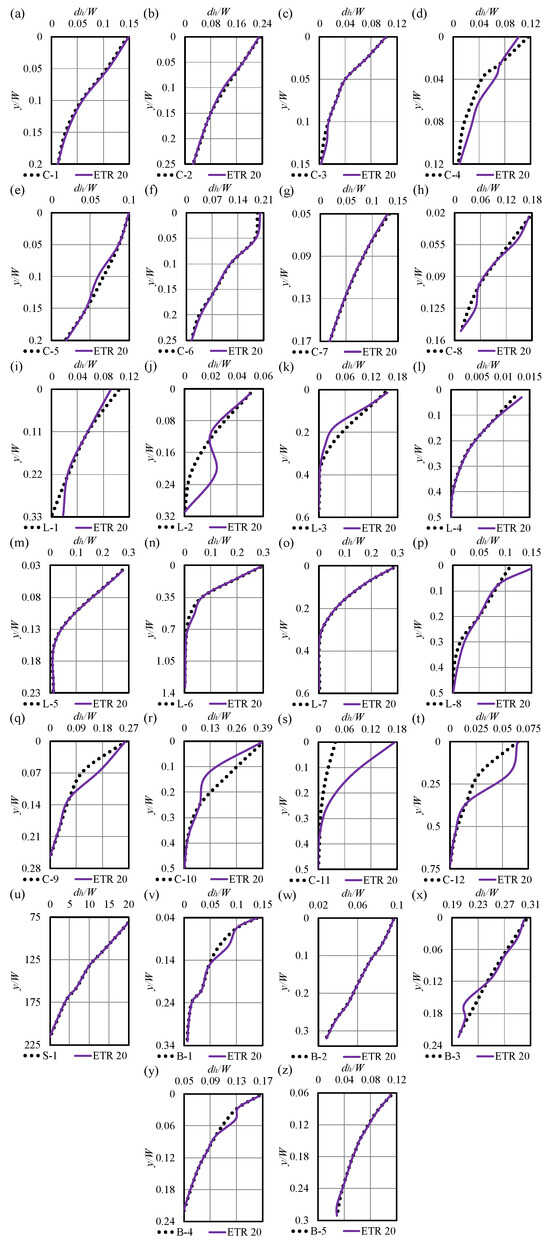
Figure 12. Horizontal deformation profiles in clay seabed simulated by ETR 20 (a–h) C-1 to C-8 (i–p) L-1 to L8 (q–t) C-9 to C-12 (u) S-1 (v–z) B-1 to B-5.

Figure 13 presents a comparison of vertical ice-scour displacements in a clay seabed, contrasting the ETR 16 model’s simulations with experimental data. Strong agreement was observed between the model and test results for cases C-1, C-2, C-3, C-7, L-1, L-3, and C-8, while deviations occurred in C-4, C-6, L-4, L-5, L-7, L-8, C-9, and B-1. The ETR 16 model predicted displacements for C-1, C-2, C-3, C-7, L-1, L-2, L-3, L-6, C-8, C-9, C-10, and C-11 using a nonlinear trend, whereas cases C-5 and C-6 followed a linear behavior.

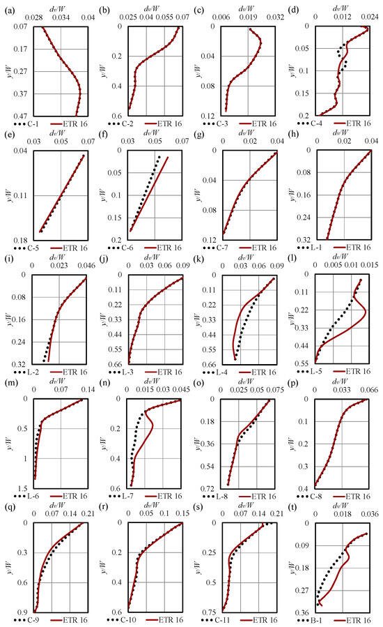
Figure 13. Vertical deformation profiles in clay seabed simulated by ETR 16 (a–g) C-1 to C-7 (h–o) L-1 to L-8 (p–s) C-8 to C-11 (t) B-1.

The ETR algorithm effectively simulated the iceberg draft and subgouge soil parameters—such as reaction forces and deformations—resulting from the iceberg tip’s impact with the seabed in both sandy and clay environments. The most accurate ETR models and key input variables were identified. These top-performing models demonstrated strong predictive ability, achieving high precision and correlation while maintaining minimal complexity.

4. Conclusions

This study aimed to develop an Extra Tree Regression (ETR) model capable of simultaneously simulating iceberg drafts and subgouge soil deformations in both sand and clay seabed, a novel application of machine learning in this field. For the first time, 22 ETR models were constructed using key parameters influencing iceberg draft prediction and subgouge soil behavior. Two extensive datasets were compiled for model training and validation, enabling the identification of optimal ETR models and the most significant input variables.

• ETR 1, incorporating all input parameters, delivered the highest accuracy in iceberg draft estimation.
• The iceberg length ratio (L/H) emerged as the most critical factor in predicting iceberg drafts using the ETR algorithm.
• The top-performing ETR models achieved exceptional accuracy, strong correlation, and computational efficiency in estimating subgouge soil parameters across both seabed types.
• For clay seabeds, the best ETR model exhibited a slight underestimation tendency but maintained the narrowest uncertainty range in predicting horizontal deformations.
• Error analysis indicated that approximately one-third of vertical displacements in clay, simulated by the leading ETR model, had errors below 16%.

As the first machine learning application to concurrently model iceberg drafts and subgouge soil characteristics, this research highlights the potential of ML in developing cost-effective, rapid solutions for safeguarding offshore infrastructure from iceberg impacts—particularly in early-stage iceberg risk management and structural design. While the results are promising, certain challenges remain, including the need for additional field and experimental data to improve model robustness and generalizability. Additionally, the current ETR framework does not provide an explicit, ready-to-use formula for practical engineering applications. Addressing these limitations will be crucial in future research to enhance the model’s real-world applicability.

Moreover, this study assumed the uniform sand and clay seabed for model training and validation. In real-world conditions, sediment layers may vary in density, cohesion, or stratification, which can influence subgouge deformation and load distribution. Future work should extend the current framework to account for non-uniform seabed conditions to better represent complex geotechnical environments and improve model transferability.

References

- Blažauskas, N.; Włodarski, M.; Paulauskas, S. Perspectives for Offshore Wind Energy Development in the South-East Baltics. Klaip. Univ. 2013, 1, 1–54. [Google Scholar] [CrossRef]
- Tsvetkova, A. The Role of Supply Vessels in the Development of Offshore Field Projects in Arctic Waters. In Arctic Marine Sustainability Arctic Maritime Businesses and the Resilience of the Marine Environment; Springer: Cham, Switzerland, 2020; pp. 249–273. [Google Scholar]
- Erokhina, O.; Mikolajewicz, U. A New Eulerian Iceberg Module for Climate Studies. J. Adv. Model. Earth Syst. 2024, 16, e2023MS003807. [Google Scholar] [CrossRef]
- Marson, J.M.; Myers, P.G.; Garbo, A.; Copland, L.; Mueller, D. Sea Ice–Driven Iceberg Drift in Baffin Bay. J. Geophys. Res. Oceans 2024, 129, e2023JC020697. [Google Scholar] [CrossRef]
- Allaire, P.E. Stability of Simply Shaped Icebergs. J. Can. Pet. Technol. 1972, 11, PETSOC-72-04-02. [Google Scholar] [CrossRef]
- Robe, R.Q.; Farmer, L.D. Physical Properties of Icebergs. Part I. Height to Draft Ratios of Icebergs. Part II. Mass Estimation of Arctic Icebergs. Coast Guard Res. Dev. Cent. 1976. [Google Scholar]
- Bass, D.W. Stability of Icebergs. Ann. Glaciol. 1980, 1, 43–47. [Google Scholar] [CrossRef]
- Hotzel, I.S.; Miller, J.D. Icebergs: Their Physical Dimensions and the Presentation and Application of Measured Data. Ann. Glaciol. 1983, 4, 116–123. [Google Scholar] [CrossRef]
- C-CORE. Documentation of Iceberg Grounding Events from the 2000 Season; C-CORE Report.: Kanata, ON, Canada, 2001; 01-C10, Revision 0. [Google Scholar]
- Barker, A.; Sayed, M.; Carrieres, T. Determination of Iceberg Draft, Mass and Cross-Sectional Areas. In Proceedings of the 14th International Offshore and Polar Engineering Conference, Toulon, France, 23–28 May 2004. [Google Scholar]
- Dowdeswell, J.A.; Bamber, J.L. Keel Depths of Modern Antarctic Icebergs and Implications for Sea-Floor Scouring in the Geological Record. Mar. Geol. 2007, 243, 120–131. [Google Scholar] [CrossRef]
- Stuckey, P.D. Drift Speed Distribution of Icebergs on the Grand Banks and Influence on Design Loads. Master’s Thesis, Memorial University of Newfoundland, St. John’s, NL, Canada, 2008. [Google Scholar]
- McKenna, R.; King, T. Modelling Iceberg Shape, Mass and Draft Changes. In Proceedings of the 20th International Conference on Port and Ocean Engineering under Arctic Conditions, Luleå, Sweden, 9–12 June 2009. [Google Scholar]
- King, T. Iceberg Interaction Frequency Model for Subsea Structures. In Proceedings of the OTC Arctic Technology Conference, Houston, TX, USA, 3–5 December 2012. OTC-23787-MS. [Google Scholar]
- Turnbull, I.D.; Fournier, N.; Stolwijk, M.; Fosnaes, T.; McGonigal, D. Operational Iceberg Drift Forecasting in Northwest Greenland. Cold Reg. Sci. Technol. 2015, 110, 1–18. [Google Scholar] [CrossRef]
- King, T.; Younan, A.; Richard, M.; Bruce, J.; Fuglem, M.; Phillips, R. Subsea Risk Update Using High Resolution Iceberg Profiles. In Proceedings of the Arctic Technology Conference, St. John’s, NL, Canada, 24–26 October 2016. OTC-27358-MS. [Google Scholar]
- Turnbull, I.D.; King, T.; Ralph, F. Development of a New Operational Iceberg Drift Forecast Model for the Grand Banks of Newfoundland. In Proceedings of the OTC Arctic Technology Conference, Houston, TX, USA, 5–7 November 2018. OTC-29109-MS. [Google Scholar]
- McKenna, R.; King, T.; Crocker, G.; Bruneau, S.; German, P. Modelling Iceberg Grounding on the Grand Banks. In Proceedings of the 25th International Conference on Port and Ocean Engineering under Arctic Conditions, Delft, The Netherlands, 9–13 June 2019; pp. 9–19. [Google Scholar]
- Stuckey, P.; Fuglem, M.; Younan, A.; Shayanfar, H.; Huang, Y.; Liu, L.; King, T. Iceberg Load Software Update Using 2019 Iceberg Profile Dataset. In Proceedings of the ASME 2021 40th International Conference on Ocean, Offshore and Arctic Engineering, Glasgow, UK, 21–30 June 2021; Volume 85178. V007T07A018. [Google Scholar]
- Azimi, H.; Mahdianpari, M.; Shiri, H. Determination of Parameters Affecting the Estimation of Iceberg Draft. China Ocean Eng. 2023, 37, 62–72. [Google Scholar] [CrossRef]
- Paulin, M.J. Preliminary Results of Physical Model Tests of Ice Scour; Memorial University of Newfoundland: St. John’s, NL, Canada; Centre for Cold Ocean Resources Engineering (C-CORE): St. John’s, NL, Canada, 1991. [Google Scholar]
- Paulin, M.J. Physical Model Analysis of Iceberg Scour in Dry and Submerged Sand; Memorial University of Newfoundland: St. John’s, NL, Canada, 1992. [Google Scholar]
- Lach, P.R. Centrifuge Modelling of Large Soil Deformation due to Ice Scour; Memorial University of Newfoundland: St. John’s, NL, Canada, 1996. [Google Scholar]
- Woodworth-Lynas, C.; Nixon, D.; Phillips, R.; Palmer, A. Subgouge Deformations and the Security of Arctic Marine Pipelines. In Proceedings of the OTC Offshore Technology Conference, Houston, TX, USA, 6–9 May 1996. OTC-8222-MS. [Google Scholar]
- C-CORE. Phase 3: Centrifuge Modelling of Ice Keel Scour; C-CORE Report.: St. John’s, NL, Canada, 1995; p. 95-Cl2. [Google Scholar]
- C-CORE. PRISE Phase 3c: Extreme LEE Gouge Event-Modeling and Interpretation; C-CORE Report.: St. John’s, NL, Canada, 1996; p. 96-C32. [Google Scholar]
- Hynes, F. Centrifuge Modelling of Ice Scour in Sand; Memorial University of Newfoundland: St. John’s, NL, Canada, 1996. [Google Scholar]
- Schoonbeek, I.S.; van Kesteren, W.G.; Xin, M.X.; Been, K. Slip Line Field Solutions as an Approach to Understand Ice Subgouge Deformation Patterns. In Proceedings of the 16th International Offshore and Polar Engineering Conference, San Francisco, CA, USA, 28 May–2 June 2006. ISOPE-I-06-289. [Google Scholar]
- Been, K.; Sancio, R.B.; Ahrabian, D.; van Kesteren, W.; Croasdale, K.; Palmer, A. Subscour Displacement in Clays from Physical Model Tests. In Proceedings of the IPC2008 7th International Pipeline Conference, Calgary, Alberta, Canada, 29 September–3 October 2008; Volume 48609, pp. 239–245. [Google Scholar]
- Yang, W. Physical Modeling of Subgouge Deformations in Sand; Memorial University of Newfoundland: St. John’s, NL, Canada, 2009. [Google Scholar]
- Arnau Almirall, S. Ice Gouging in Sand and the Associated Rate Effects; University of Aberdeen: Aberdeen, UK, 2017. [Google Scholar]
- Kioka, S.D.; Kubouchi, A.; Saeki, H. Training and Generalization of Experimental Values of Ice Scour Event by a Neural-Network. In Proceedings of the 13th International Offshore and Polar Engineering Conference, Honolulu, HA, USA, 25–30 May 2003. ISOPE-I-03-081. [Google Scholar]
- Kioka, S.; Kubouchi, A.; Ishikawa, R.; Saeki, H. Application of the Mechanical Model for Ice Scour to a Field Site and Simulation Method of Scour Depths. In Proceedings of the 14th International Offshore and Polar Engineering Conference, Toulon, France, 23–28 May 2004. ISOPE-I-04-107. [Google Scholar]
- Azimi, H.; Shiri, H. Dimensionless Groups of Parameters Governing the Ice-Seabed Interaction Process. J. Offshore Mech. Arctic Eng. 2020, 142, 051601. [Google Scholar] [CrossRef]
- Azimi, H.; Shiri, H. Ice-Seabed Interaction Analysis in Sand Using a Gene Expression Programming-Based Approach. Appl. Ocean Res. 2020, 98, 102120. [Google Scholar] [CrossRef]
- Azimi, H.; Shiri, H. Assessment of Ice-Seabed Interaction Process in Clay Using Extreme Learning Machine. Int. J. Offshore Polar Eng. 2021, 31, 411–420. [Google Scholar] [CrossRef]
- Azimi, H.; Shiri, H.; Zendehboudi, S. Ice-Seabed Interaction Modeling in Clay by Using Evolutionary Design of Generalized Group Method of Data Handling. Cold Reg. Sci. Technol. 2022, 193, 103426. [Google Scholar] [CrossRef]
- Azimi, H.; Shiri, H.; Mahdianpari, M. Simulation of Subgouge Sand Deformations Using Robust Machine Learning Algorithms. In Proceedings of the OTC Offshore Technology Conference, Houston, TX, USA, 2–5 May 2022. OTC-31937-MS. [Google Scholar]
- Azimi, H.; Shiri, H.; Mahdianpari, M. Iceberg-Seabed Interaction Evaluation in Clay Seabed Using Tree-Based Machine Learning Algorithms. J. Pipeline Sci. Eng. 2022, 2, 100075. [Google Scholar] [CrossRef]
- Geurts, P.; Ernst, D.; Wehenkel, L. Extremely Randomized Trees. Mach. Learn. 2006, 63, 3–42. [Google Scholar] [CrossRef]
- Hammed, M.M.; AlOmar, M.K.; Khaleel, F.; Al-Ansari, N. An Extra Tree Regression Model for Discharge Coefficient Prediction: Novel, Practical Applications in the Hydraulic Sector and Future Research Directions. Math. Probl. Eng. 2021. [Google Scholar] [CrossRef]
- El-Tahan, M.; El-Tahan, H.; Courage, D.; Mitten, P. Documentation of Iceberg Groundings; Environmental Studies Revolving Funds report; Environmental Studies Revolving Funds: Ottawa, ON, Canada, 1985; Volume 7. [Google Scholar]
- Woodworth-Lynas, C.M.T.; Simms, A.; Rendell, C.M. Iceberg Grounding and Scouring on the Labrador Continental Shelf. Cold Reg. Sci. Technol. 1985, 10, 163–186. [Google Scholar] [CrossRef]
- Løset, S.; Carstens, T. Sea Ice and Iceberg Observations in the Western Barents Sea in 1987. Cold Reg. Sci. Technol. 1996, 24, 323–340. [Google Scholar] [CrossRef]
- McKenna, R. Development of Iceberg Shape Characterization for Risk to Grand Banks Installations; PERD/CHC Report; National Research Council Canada: Ottawa, ON, Canada, 2004; p. 20473.
- Sonnichsen, G.; Hundert, T.; Myers, R.; Pocklington, P. Documentation of Recent Iceberg Grounding Events and a Comparison with Older Events of Known Age; Environmental Studies Research Funds: Ottawa, ON, Canada, 2006; Volume 157.
- McGuire, P.; Younan, A.; Wang, Y.; Bruce, J.; Gandi, M.; King, T.; Keeping, K.; Regular, K. Smart Iceberg Management System–Rapid Iceberg Profiling System. In Proceedings of the OTC Arctic Technology Conference, St. John’s, NL, Canada,, 24–26 October 2016. OTC-27473-MS. [Google Scholar]
- Younan, A.; Ralph, F.; Ralph, T.; Bruce, J. Overview of the 2012 Iceberg Profiling Program. In Proceedings of the OTC Arctic Technology Conference, St. John’s, NL, Canada, 24–26 October 2016. OTC-27469-MS. [Google Scholar]
- Talimi, V.; Ni, S.; Qiu, W.; Fuglem, M.; MacNeill, A.; Younan, A. Investigation of Iceberg Hydrodynamics. In Proceedings of the OTC Arctic Technology Conference, St. John’s, NL, Canada, 24–26 October 2016. OTC-27493-MS. [Google Scholar]
- Zhou, M. Underwater Iceberg Profiling and Motion Estimation Using Autonomous Underwater Vehicles. Ph.D. Thesis, Memorial University of Newfoundland, St. John’s, NL, Canada, 2017. [Google Scholar]
Disclaimer/Publisher’s Note: The statements, opinions and data contained in all publications are solely those of the individual author(s) and contributor(s) and not of MDPI and/or the editor(s). MDPI and/or the editor(s) disclaim responsibility for any injury to people or property resulting from any ideas, methods, instructions or products referred to in the content. |
© 2025 by the authors. Licensee MDPI, Basel, Switzerland. This article is an open access article distributed under the terms and conditions of the Creative Commons Attribution (CC BY) license (https://creativecommons.org/licenses/by/4.0/).