Empirical Modelling of Ice-Jam Flood Hazards Along the Mackenzie River in a Changing Climate

Abstract

This study introduces a novel methodology for assessing ice-jam flood hazards along river channels. It employs empirical equations that relate non-dimensional ice-jam stage to discharge, enabling the generation of an ensemble of longitudinal profiles of ice-jam backwater levels through Monte-Carlo simulations. These simulations produce non-exceedance probability profiles, which indicate the likelihood of various flood levels occurring due to ice jams. The flood levels associated with specific return periods were validated using historical gauge records. The empirical equations require input parameters such as channel width, slope, and thalweg elevation, which were obtained from bathymetric surveys. This approach is applied to assess ice-jam flood hazards by extrapolating data from a gauged reach at Fort Simpson to an ungauged reach at Jean Marie River along the Mackenzie River in Canada’s Northwest Territories. The analysis further suggests that climate change is likely to increase the severity of ice-jam flood hazards in both reaches by the end of the century. This methodology is applicable to other cold-region rivers in Canada and northern Europe, provided similar fluvial geomorphological and hydro-meteorological data are available, making it a valuable tool for ice-jam flood risk assessment in other ungauged areas.

1. Introduction

1.1. Importance of Ice-Jam Flood Hazard Assessment

Ice-jam flood hazard assessment is particularly important due to the unique and complex nature of ice-jam events, common occurrences on many northern and cold-region river systems, which differ significantly from typical open-water floods. These floods occur when ice accumulates and obstructs river flow, causing a sudden and often extreme rise in upstream water levels. Despite relatively low discharge rates, ice jams can produce some of the highest recorded flood stages, making them especially hazardous.

Ice-jam flood hazard assessment is essential for understanding the flood risks posed by ice-related flooding events. Ice-jam flood hazard assessment involves evaluating the likelihood and severity of flooding caused by ice jams. This process requires analyzing historical data, hydrological and hydraulic conditions, and river morphology to estimate the probability and potential impact of ice-jam-induced flooding. By identifying areas where ice jams are likely to form and assessing the resulting water levels and flood extents, hazard assessments can support informed decision-making for infrastructure planning, emergency preparedness, and community safety. These assessments also help determine the vulnerability of critical assets and populations to ice-jam events, guiding the development of mitigation strategies such as ice control structures or operational responses such as ice breaking and flood forecasting.

Furthermore, ice-jam flood hazard assessments are increasingly important in the context of climate change, which is expected to alter freeze–melt cycles, river ice dynamics, and precipitation patterns. Understanding how these changes influence ice-jam formation and flood potential enables communities to adapt and build resilience against future flood risks.

1.2. Challenges in Hazard Assessment of Ice-Jam Floods Compared to Open-Water Floods

Ice-jam flood hazard assessment requires a distinct approach from that used for open-water floods due to fundamental differences in their mechanisms, timing, and predictability. While open-water floods are typically driven by high flows resulting from rainfall, snowmelt, and soil saturation, often occurring in spring and summer, ice-jam floods are caused by the accumulation of ice that obstructs river flow. This obstruction can occur during freeze-up in early winter, spring breakup, or even during mid-winter freeze–melt cycles, leading to a rapid rise in upstream water levels despite relatively low discharges.

The unpredictability of ice-jam floods stems from the complex interactions between river flow and ice dynamics, including the formation, stalling (jamming), and sudden release (javes = ice-jam release waves) of ice accumulations. These processes make it difficult to anticipate the timing, location, and severity of ice-jam events. Assessing the hazard posed by such events involves understanding not only hydrological conditions but also ice characteristics such as thickness, strength, and volume, parameters that are highly variable and challenging to measure.

Unlike open-water floods, ice-jam floods can affect areas that are not typically considered flood-prone, and they often develop rapidly and unpredictably. This “flashy” behavior, combined with the potential for nighttime (colder air temperatures) occurrence, poses significant challenges for emergency response and community safety. In addition to high water levels, ice impacts and ride-up onto shorelines can damage infrastructure and buildings, which must be accounted for in hazard assessments. Ice-jam floods may be an added contributor to riverbank erosion and can alter flow patterns and sediment transport, impacting riverine ecosystems.

Debris-related floods are also unpredictable and difficult to model, especially when debris accumulates at river bends or crossings. While woody debris floods may occur in smaller, confined channels, typically in rivers of stream order 1 or 2, for example, in Buffalo Creek [1], larger rivers like the Mackenzie are generally too wide for such debris to cause jamming and significant flooding. Even though the Liard River contributes substantial woody debris to the Mackenzie at Fort Simpson (pers. comm. Natalie Kramer Anderson), the scale of the Mackenzie reduces the likelihood of debris-induced blockages leading to flooding.

1.3. Reach-Based Extrapolation Using Empirical Approach (Adapted from [2] )

Many communities along rivers in the Northwest Territories lack water-level and flow gauges, making ice-jam flood hazard assessment particularly challenging at those locations. One such community is Jean Marie River, which lies along the Mackenzie River. Although this community does not have a gauge, a gauge is located 68 km downstream at Fort Simpson, allowing for the possibility of extrapolating ice-jam flood hazard assessments from the gauged to the ungauged reach. Such a reach-based extrapolation approach has been applied in other river systems, such as from Fort McMurray to Fort MacKay on the Athabasca River [2] and Fort Simpson to Jean Marie River [3]. However, these examples only demonstrate the feasibility of transferring ice-jam flood hazard assessments from a single point along the river (at a gauge) to another point along the river (point of interest at an ungauged river section). In this study, we extend the approach by extrapolating not just from one point to another but longitudinal profiles of ice-jam flood hazard from one river reach to another.

Extrapolating ice-jam flood hazards to ungauged areas presents significant challenges due to data limitations. To address this, an empirical method based on non-dimensional stage and discharge relationships has been used. This approach requires only a minimal set of fluvial geomorphological data, primarily river width and slope, which can be derived from digital terrain models. However, estimating thalweg elevations remains more difficult, as these are typically obtained through under-ice flow measurements and bathymetric surveys. In this study, a bathymetric survey conducted at Fort Simpson provided the necessary data on river width, slope, and bed elevation. These parameters enabled the assessment of ice-jam flood hazard at Fort Simpson, which could then be extrapolated to Jean Marie River. To complete the extrapolation, a back-calculation using Manning’s equation was required to estimate the thalweg elevations at the ungauged site.

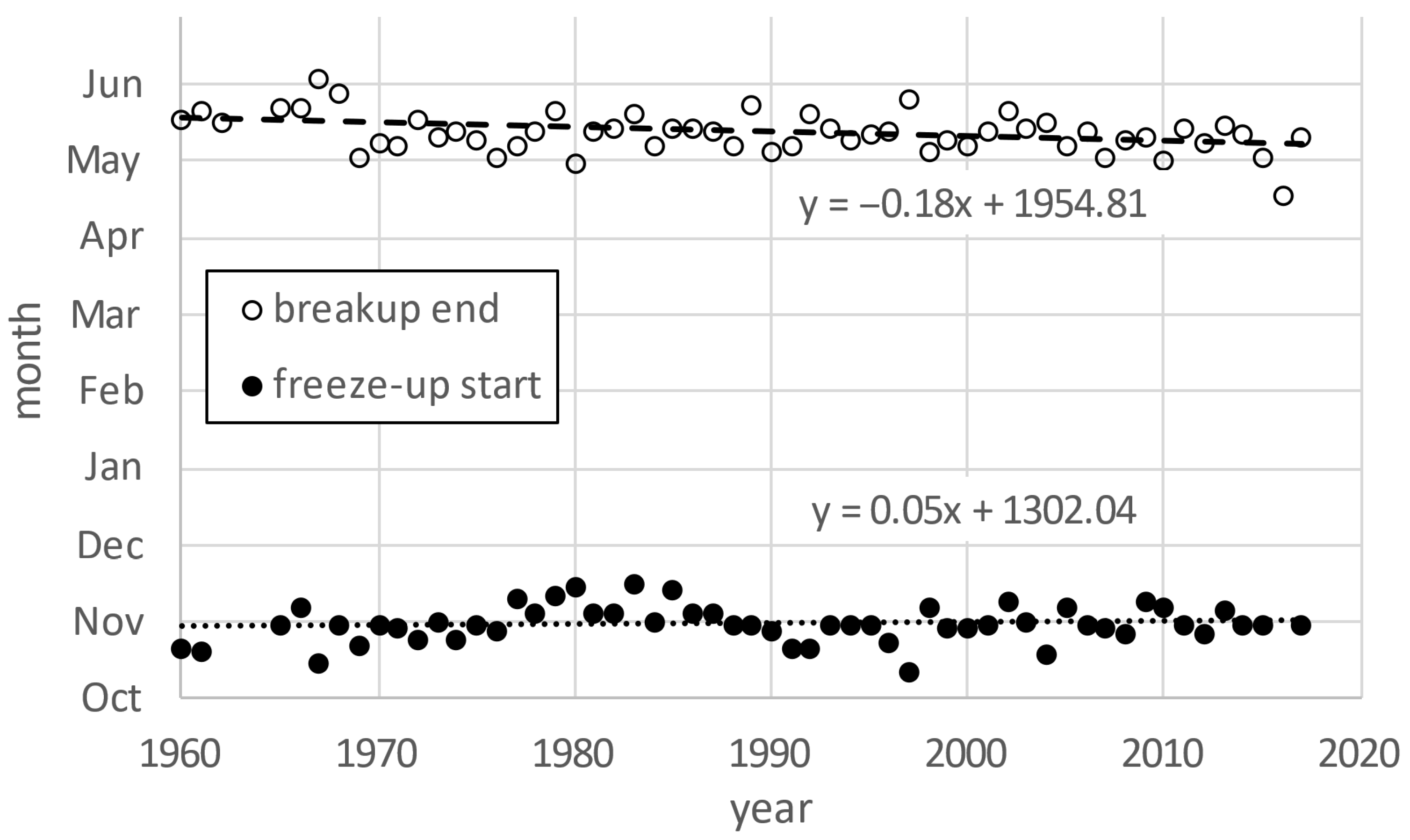
1.4. Shifts in Ice-Jam Flood Hazard Due to Climate Change

Climate change adds complexity to ice-jam flood hazard assessment by altering river ice regimes. Rising air temperatures and changing precipitation patterns are expected to shift the timing and frequency of freeze-up and breakup events, increasing the likelihood of mid-winter breakup and modifying the seasonal dynamics of ice-jam formation. These evolving conditions must be integrated into hazard assessments to ensure communities are prepared for future risks.

Climate change can affect river-ice phenology, thickness, and flood potential by altering air temperature and precipitation patterns, leading to changes in hydrological regimes and impacting ice-jam flood frequency and magnitude [4]. This poses concerns for property developers, insurance companies, government agencies, and riverine communities, requiring effective planning and flood mitigation measures.

Robust modeling frameworks that incorporate future climatic changes are necessary to produce reliable ice-jam flood hazard scenarios. However, modeling frameworks to better establish the impacts of climate change on future ice jams and ice-jam flooding still require further advancement [5]. Reliable methods for assessing future ice-jam flood risk are essential for effective water resources planning and management. Estimating future ice-jam flood hazards helps evaluate the adequacy of existing flood protection systems and allocate resources efficiently for future mitigation programs [6,7]. A sustainable ice-jam flood management strategy should address both current and future hydroclimatic impacts to ensure maximum flood protection and preserve natural ecosystems.

Recent studies have introduced various methods of quantifying future climate impacts on ice regimes, from simplified empirical methods using projected air temperature data from global circulation models [8] to physics-based hydrodynamic models [7,9] and hydrology-hydraulic model couplings [10,11]. The latter approaches require extensive hydro-meteorological data and historical ice jam information, while simpler approaches are well-suited for data-sparse study sites. Understanding the timing and magnitude of runoff under future climatic conditions is paramount for estimating impacts of future climate on ice-jam hazard. Hydrological models, driven by climatic scenarios, can generate future hydrological conditions which must replicate relevant hydrological indicators to assess future flow conditions accurately [12,13].

The present study focuses on shifts in ice-jam flood hazard due to changes in the climate at Fort Simpson and Jean Marie River along the Mackenzie River. Future air temperature and flow scenarios derived from a basin-wide hydrological model of the Mackenzie River basin form the basis for determining the impact of climate change on ice-jam flood hazard. The changes are calculated for both communities to provide insight into the ways climate change may alter ice-jam flood hazard, which can be used as a basis for planning and developing effective flood mitigation strategies.

1.5. Objectives

Under the Canadian government’s Flood Hazard Identification and Mapping Program (FHIMP), several federal agencies are collaborating with provinces and territories to address flood risks in vulnerable communities. In alignment with this national initiative, the Government of the Northwest Territories (GNWT) is conducting work to assess flood hazards in communities such as Fort Simpson and Jean Marie River along the Mackenzie River. Within this broader context, the specific focus of this study is on assessing the hazard posed by ice-jam flooding in these regions, aiming to better understand the likelihood, severity, and potential impacts of such events to support risk reduction and resilience planning.

(1)

Assessing ice-jam flood hazard along the Fort Simpson reach: This objective builds on previous work [3] involving reach-based extrapolation of ice-jam flood hazards by extending the assessment beyond a single gauge location to the entire river reach at Fort Simpson. Using an empirical approach [14,15] embedded within a Monte-Carlo framework, the method simulates ensembles of backwater profiles based on probabilistic distributions of ice-jam lodgment locations. From these simulations, annual exceedance probability (AEP) profiles, particularly the 1:100 and 1:200 AEP levels, are derived to characterize the severity and likelihood of ice-jam flooding along the reach.

(2)

Transferring ice-jam flood hazard assessment to ungauged reaches: This objective focuses on extrapolating the ice-jam flood hazard assessment from the gauged reach at Fort Simpson to the ungauged reach at Jean Marie River. By applying the same empirical and probabilistic framework, the study aims to estimate flood hazard levels in a data-sparse region, enabling hazard characterization in communities without direct gauge measurements.

(3)

Evaluating climate-driven shifts in ice-jam flood hazard: Building on recent research [16] this objective assesses how climate change may alter ice-jam flood hazards at both Fort Simpson and Jean Marie River. The analysis considers projected changes in freeze–melt cycles, river ice dynamics, and hydrological conditions to estimate future shifts in the frequency and severity of ice-jam flooding.

2. Description of Study Sites (Excerpts and Adaptations from [17])

Two study sites were chosen along the Mackenzie River (see Figure 1):

-

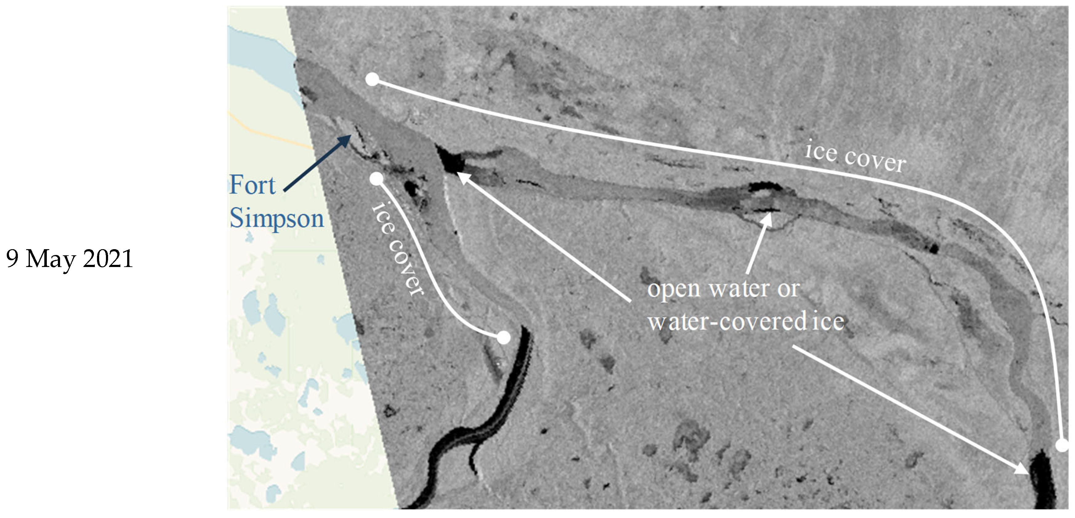
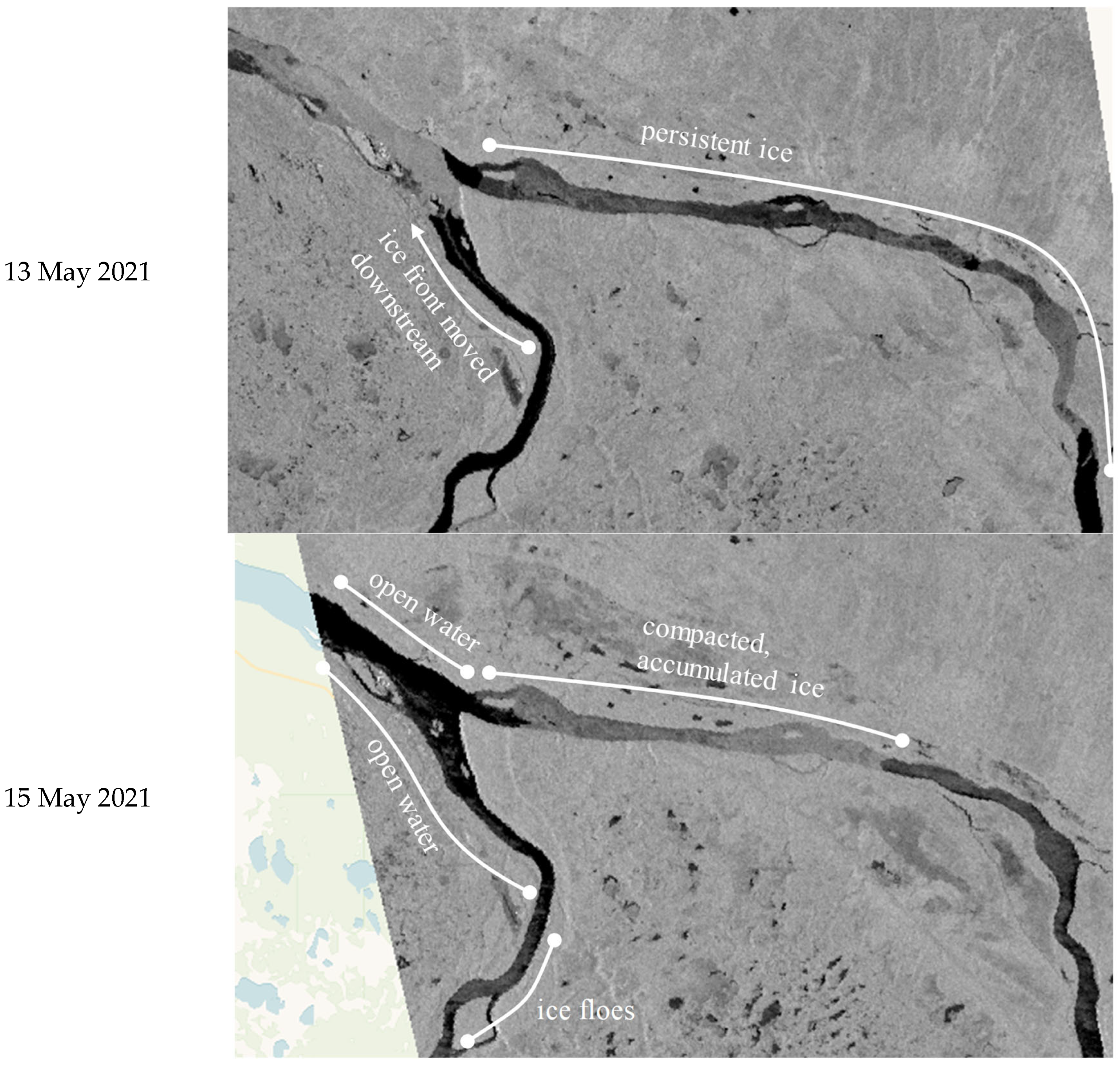
Fort Simpson (gauged site): Fort Simpson lies approximately 300 km downstream of Great Slave Lake with a water surface elevation drop of about 32 m from the lake (approximated from Google Earth; very flat river, 0.0107% slope). The village is situated on the south shore of the Mackenzie River, just downstream of the Liard River outflow into the Mackenzie River. A gauge is situated on the Liard River just upstream of its confluence.

-

Jean Marie River (ungauged site): Jean Marie River is located approximately 68 km upstream of Fort Simpson along the Mackenzie River. The community is situated on the south shore of the Mackenzie River, just upstream of the Jean Marie River outflow into the Mackenzie River. This tributary is a few stream orders smaller than the Liard River outflow at Fort Simpson; hence, it may have less impact on the Mackenzie River flow and ice regimes than the Liard River. A flow gauge is situated on Jean Marie River but a substantial distance upstream of the confluence.

Both communities experience floods caused by ice jams during the spring breakup of the river’s ice cover. Severe ice jams occurred along both communities during the spring breakup of 2021, causing extensive flooding in each.

River Ice Dynamics

The freeze-up and end-of-breakup dates at the Fort Simpson gauge (gauge ID 10GC001) from 1960 to 2018 show a slight trend towards earlier end-of-breakup dates by approximately 18 days over a 100-year period, while freeze-up dates remain relatively constant with only a slight trend towards later dates, by 5 days over the same period (see Figure 2). The b-flags that accompany the daily flow readings indicate ice-influenced water-level recordings marking, respectively, the beginning and end of the river’s freeze-up and breakup periods. A similar analysis at the gauge at Strong Point (gauge ID 10FB006) from 1991 to 2018 aimed to determine if breakup occurred earlier upstream of Fort Simpson. However, the analysis by Lindenschmidt [17] showed that an ice cover and its breakup can still persist upstream of Fort Simpson even if the Mackenzie River is already clear of ice at Fort Simpson. A b-flag analysis for the Liard River near its mouth compared 45 years (1973–2017) of breakup end dates recorded at the gauges at Fort Simpson and the Liard River mouth. The ice cover in the vicinity of the mouth of the Liard River persisted longer than the ice at Fort Simpson for only 5 years out of the 45-year series.

During the 10 May 2021 ice-jam flood event, extensive flooding occurred in Fort Simpson. The European Space Agency’s Sentinel-1 space-borne remote sensing images (Figure 3) acquired on 9 May 2021, a day before the event, and on 13 and 15 May 2021, several days after the maximum staging occurred, show substantial ice cover along the Mackenzie River upstream of Fort Simpson. The ice cover extended approximately 10 km upstream of the Liard River from its mouth. The ice cover upstream of the Mackenzie and Liard River confluence persisted throughout the event, and the additional Liard River ice contributed to the severe jamming at Fort Simpson on 10 May 2021. Even when the ice cleared out along the Liard River mouth and the Fort Simpson reach along the Mackenzie River, an ice cover remained lodged upstream of the Mackenzie/Liard River confluence on 15 May 2021. This indicates that the ice source for jamming at Fort Simpson can also stem from the Liard River and that the complete breakup of the ice cover along the Mackenzie River upstream of Fort Simpson can persist even when the river is clear of ice at and downstream of Fort Simpson.

Jean Marie River, situated upstream of Fort Simpson along the Mackenzie River, also faces the threat of ice-jam floods during the spring breakup. The ice cover in the vicinity of the mouth of the Liard River has been observed to persist longer than the ice at Fort Simpson in some years, contributing to severe ice jamming downstream at Fort Simpson.

The flow in the upper Mackenzie River from Great Slave Lake is highly dependent on the water levels in the lake. Higher water levels in Great Slave Lake result in increased discharge into the upper Mackenzie River. This increased flow can exacerbate the spring breakup process and lead to more severe ice jams and flooding downstream [18].

Simulated rating curves for open-water and ice-covered conditions in the spring of 1992 along the South Channel (South of Big Island) at the outlet of Great Slave Lake show that the lake ice thickness plays a crucial role in determining discharge rates. For instance, in late April 1992, the ice thickness at the South Channel was measured to be approximately 0.6 m [19]. Simulations indicate that varying ice thickness can significantly impact discharge, with thicker ice reducing flow and thinner ice increasing it. This relationship highlights how the physical state of the lake’s ice cover can influence the volume of water flowing into the Mackenzie River during spring breakup [18].

Furthermore, climate change is expected to alter these dynamics. Thinner ice covers in the future, resulting from warmer temperatures, could potentially increase the outflow from Great Slave Lake. However, this increase might be offset by overall lower water levels in the lake due to a warmer climate, which could lead to lower annual minimum lake levels in the fall and reduced annual maximum water levels. An example of this would be the low-water year of 2024. The interplay between these factors requires further detailed study to understand the compensatory effects [18].

The water level elevations recorded at Yellowknife from 1938 to mid-2021 show significant variability, with peaks in the early 1960s and in September 2020. These high-water levels can contribute to increased flows during spring breakup, potentially leading to severe ice-jam flooding events, as observed in Fort Simpson in 2021. The dependence of the upper Mackenzie River’s flow on Great Slave Lake’s water levels underscores the importance of monitoring and understanding these dynamics to predict and manage ice-jam flood risks effectively.

3. Methodology

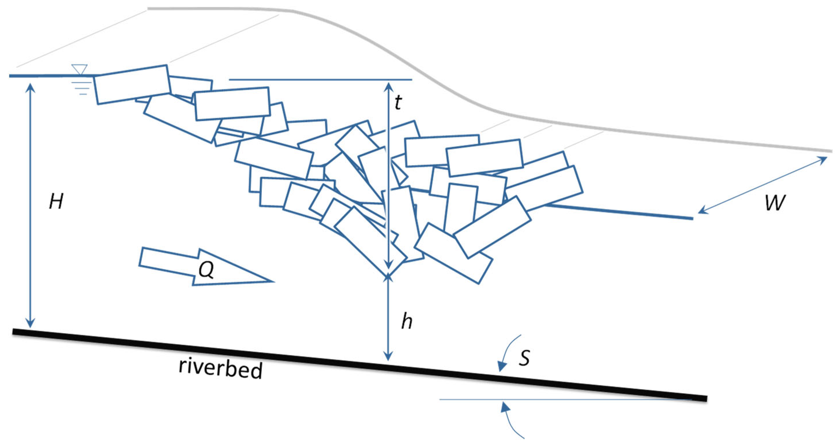
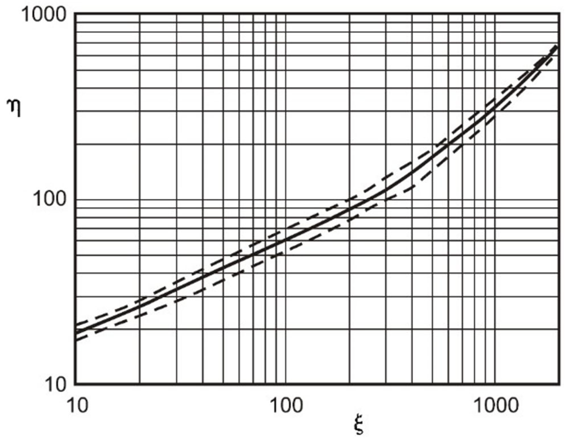
3.1. Empirical Model (Adapted from [3])

In this study, an empirical approach was used to calculate equilibrium ice-jam backwater levels. The analytical method stems from Beltaos [14,15] and has been extended [2] in an ice-jam flood prediction context. Referring to Figure 4, from a dimensional analysis, the dimensionless discharge ξ and dimensionless ice-jam stage η can be determined:

$$\xi ={\displaystyle \frac{{\left(\frac{{\left[\frac{Q}{W}\right]}^2}{gS}\right)}^{1/3}}{WS}}$$

(1)

$$\eta ={\displaystyle \frac{H}{WS}}$$

(2)

where g is the gravitational acceleration (m/s²), H is the backwater staging depth (m), Q is the discharge (m³/s), S is the slope (-) and W is the river width (m).

Rearranging Equation (2), where H is a function of η, W and S, yields:

$$H=\eta ·W·S$$

(3)

The relationship between ξ and η is shown graphically in Figure 5, which includes a confidence band to reflect the range of variation within ξ and η due to differences in ice characteristics and fluvial geomorphology.

The equation for η can be extended to

$$\eta ={\displaystyle \frac{H}{WS}}=0.63f_o^{1/3}\xi +{\displaystyle \frac{5.75}{\mu }}\left(1+\sqrt{1+0.11\mu f_o^{1/3}\left({\displaystyle \frac{f_i}{f_o}}\right)\xi }\right)$$

(4)

“where f_o is a composite friction factor calculated from the average of the ice friction factor f_i and the riverbed friction factor f_b and μ is a coefficient. The parameter μ is the friction coefficient and represents the internal strength of the ice cover. This coefficient is a lumped variable representing the effects of several unknowns or difficult-to-determine factors, including lateral stress within the ice cover, ice on bank friction, angle of internal resistance, porosity, and possibly cohesion.

Table 1. Typical ranges of f_o, f_i/f_o and μ for different riverbed slopes compiled from [2,14].

Slope (–)	fo	fi/fo	μ	Example Sites
0.0001–0.0003	<0.1	1.4–1.5	1.2–1.3	Thames River; Churchill River (Labrador)
0.0003–0.0004	0.3–0.4	1.3–1.7	0.8–1.6	Athabasca River near Fort McMurray; upper Dauphin River; Red River
0.0007–0.0010	0.1–0.7	0.6–1.5	0.6–1.2	Smoky River; Athabasca River upstream of Fort McMurray; lower Dauphin River

shows typical ranges of these parameters for various riverbed slopes” [2,21].

The depth h (m) of water under the ice jam can be calculated using [14]

$$h={\left[{\displaystyle \frac{q}{{\left(\frac{4gS}{f_o}\right)}^{1/2}}}\right]}^{2/3}$$

(5)

and the maximum thickness t (m) of the ice jam is

$$t={\displaystyle \frac{H-h}{s_i}}$$

(6)

where s_i is the specific gravity of ice (= 0.92).

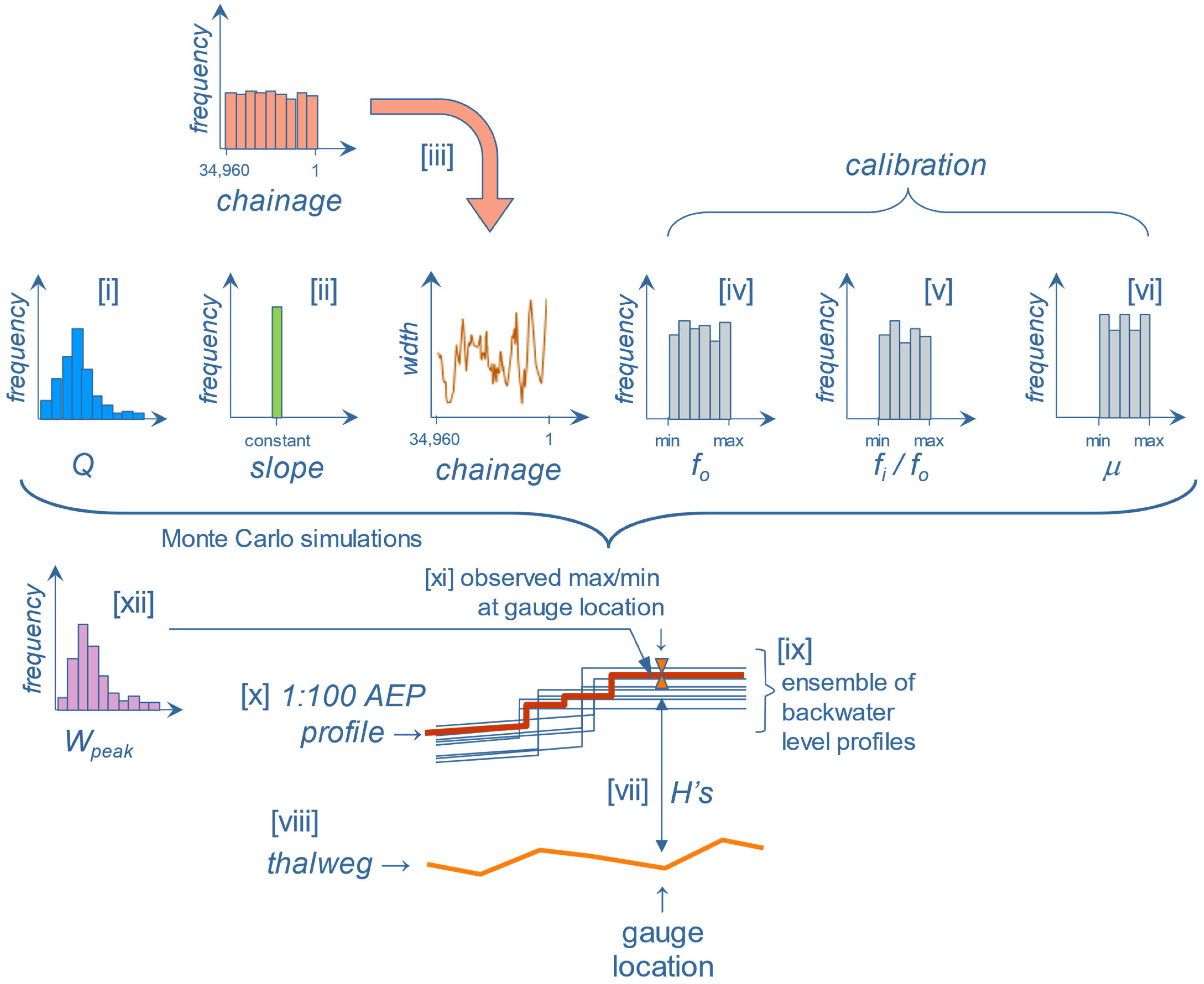
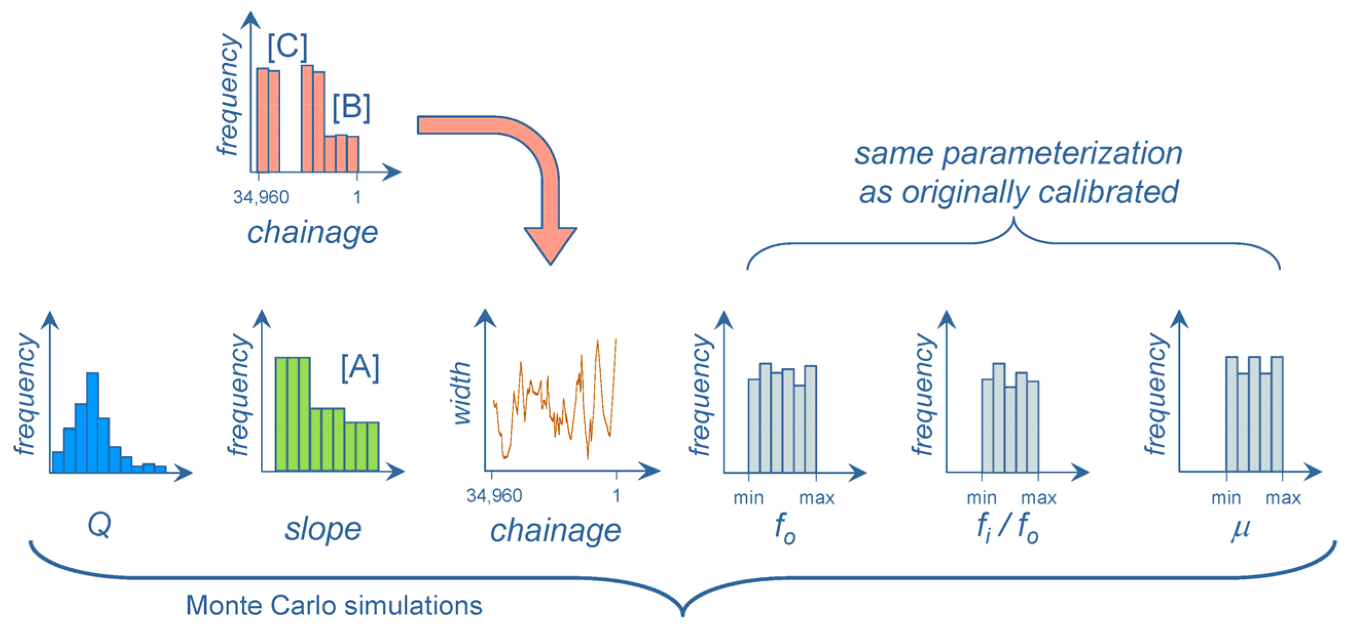
3.2. Monte-Carlo Framework

The Monte-Carlo framework was improved by extending it, not to just considering ice-jam flood hazard at one point as in the conceptualization above but, to consider ice-jam flood hazard at all points along the entire chainage of the reach. This is represented by using points along a centerline, to create ensembles of longitudinal profiles of ice-jam flood hazard. Referring to Figure 6, the same extreme value distribution of flows derived from the gauge data was used (see [i] in Figure 6). The same constant slope value at the site, derived from the bathymetric survey, was applied (see [ii] Figure 6). The bathymetry also yielded widths along the river reach. For each Monte-Carlo run, a chainage was randomly chosen, from which a width was read from the width = f(chainage) relationship (see [iii] in Figure 6). The parameters f_o, f_i/f_o and μ (see [iv], [v] and [vi] in Figure 6, respectively) required adjustment to reflect the differences in ice-cover characteristics along the reach compared to just one point (at the gauge).

The Monte-Carlo Analysis yielded an ensemble of backwater depths H (see [vii] in Figure 6) which were added to the thalweg elevation (see [viii] in Figure 6 to each corresponding chainage.

3.3. Creation of Ice Jam Profiles

In order to create ice-jam profiles (see [ix] in Figure 6), for each profile, the backwater elevation was extended from its chainage in the upstream direction (see [a] in Figure 7). The profile upstream of the jam should slope upward; however, the length of the ice jam cannot be calculated. Hence, the backwater profile was assumed to remain horizontal, which may introduce an underestimate of the hazard profiles. This underestimate can be compensated for by slight increases in the calibration values of the friction coefficients.

The water-level profile downstream from the chainage location runs parallel to the thalweg slope (see [b] in Figure 7). The elevation of the downstream portion of the profile is such that it can pass through the elevation determined from the derived under-ice rating curve at the gauge (see Figure 8). The two profiles are then combined to form an ice-jam profile (see [c] in Figure 7).

The process is repeated 100s of times to yield an ensemble of ice-jam profiles (see [d] in Figure 7). The profile ensemble can be summarized using percentiles of the water-level elevations at each chainage. For instance, the 99th percentile corresponds to the 1:100 AEP (indicated by [x] in Figure 6 and [e] in Figure 7). The parameters f_o, f_i/f_o and μ (respectively, [iv], [v] and [vi] in 6) are adjusted until the percentile profiles ([x] in Figure 6) pass through the corresponding observed return period (see [xi] in Figure 6 and [f] in Figure 7), which are derived from the water-level elevations recorded at the gauge (see [xii] in Figure 6).

3.4. Incorporating Reach-Based Extrapolation

The ice-jam flood hazard assessment of Fort Simpson (gauged reach) was extrapolated to Jean Marie River (ungauged reach) to provide an initial assessment of that community’s current and future potential flood hazard due to ice jams. The methodology of the extrapolation has been reported in Lindenschmidt et al. [3] but a summary is warranted here. A Monte-Carlo Analysis framework was applied for the gauged reach to calculate the non-dimensional discharge and stages many thousands of times using random values of input parameters extracted from frequency distributions. These parameters include an extreme value distribution of the flows at the end of breakup, a constant slope value from elevation data, a uniform distribution of river widths, and uniform distributions of the ice parameters f_o, f_i/f_o and μ. The simulations yield backwater depths, which were added to the thalweg elevation derived from the maximum depth recorded by acoustic doppler current profiler (ADCP) data and water-level elevation at the time of the ADCP survey. This resulted in an ensemble of backwater level elevations. Percentiles of these elevations correspond to return periods, which are graphed to calculate a hazard curve. The calculated hazard curve must lie between the observed minimum and maximum hazard curves derived from the extreme value distribution of instantaneous backwater level elevation maxima recorded at the gauge. The ranges of the distributions of the parameters are adjusted until the calculated hazard curve lies within the observed range of hazard curves.

The Monte-Carlo framework for the gauged reach was then applied to the ungauged reach by transferring most of the parameterizations, with a few adjustments to fit the conditions of the ungauged site. The same extreme value distribution of flows is used, except for Jean Marie River, where the frequency distribution of flows recorded at Strong Point is used. (In this study, a distribution of the fraction of flow at Strong Point compared to Fort Simpson was determined and applied to the Fort Simpson flows to estimate the flows at Jean Marie River, both for current and future climate-impacted ice-jam flood hazard assessments at Jean Marie River; this simplified approach is preferred since the uncertainty in the thalweg elevation, described next, overshadows the uncertainty in the flow distributions). A constant slope value from the digital terrain model at the site was applied. The range of widths was adjusted to those observed at the ungauged site. The same ranges of the f_o, f_i/f_o and μ parameters were maintained. The Monte-Carlo Analysis yielded an ensemble of backwater depths, which were added to the thalweg elevation, an elevation increment corresponding to the difference in water-level surface elevations between the gauged and ungauged sites. This represents a high level of uncertainty since the river depths at the two sites for the same flow conditions are not necessarily similar. (In this study, Manning’s equation was used to back calculate the thalweg elevation from Fort Simpson to estimate the thalweg elevation at Jean Marie River.) The backwater level depths are then added to the thalweg elevation to yield an ensemble of backwater level elevations, from which return periods can be estimated to predict a hazard curve for the ungauged reach.

3.5. Incorporating Climate-Change Impacts

Shifts in ice-jam flood hazard at Fort Simpson due to climate change have been investigated [16], but a brief summary of the methodology is warranted here, where a hydrological model is used as the reference of flow values, and the cumulative degree days of melting (CDDMs) are used to find the breakup timing

The core components of the work are the following:

-

CDDM is used to estimate breakup timing

-

MESH provides modeled flows

-

Climate models (CanRCM4-ESM2) provide future temperatures

-

bias correction is applied

-

Breakup dates are adjusted based on observed timing trends

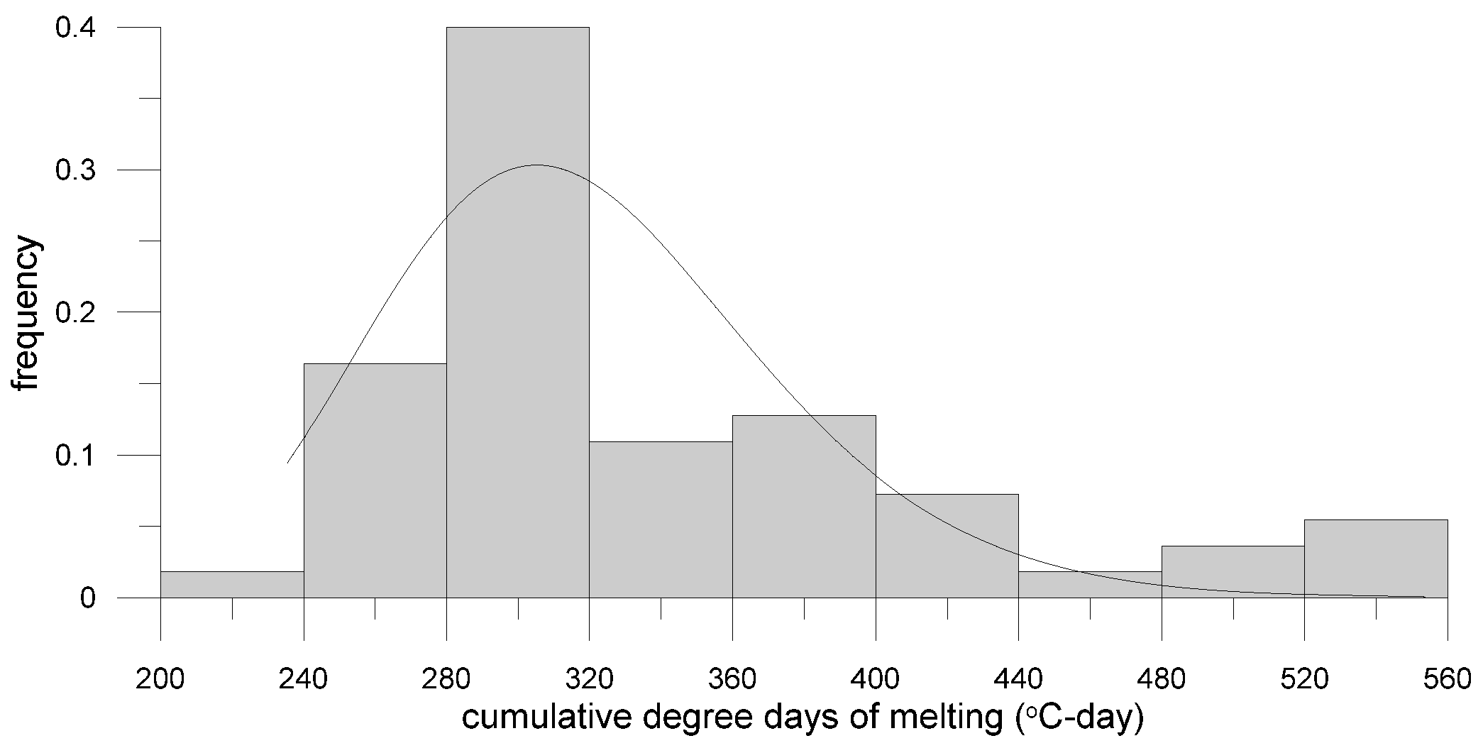
3.5.1. Step 1: Historical CDDM Calculation and Distribution

The cumulative degree days of melting (CDDM) were computed to examine the thermal energy buildup that causes ice breakup events. The CDDM were determined to measure the amount of ice melting during the pre-breakup to breakup period (1 April–31 May) using:

$$CDDM=\sum _{i=D_1}^{D_n}(T_{Di}+5)$$

where D₁ is the starting day for calculating CDDM, T represents the daily mean air temperature (from the meteorological station at Fort Simpson), and an additional 5 °C is included to account for the contribution of solar radiation to ice melting. The CDDM values at the end of breakup period starting 1 April to the last date of b-flag (The b-flag indicates ice-influenced water-level recordings and is marked beside flow readings when discharge is affected by backwater from ice covering the river at or near the gauge. The first b-flag of winter marks the start of freeze-up, while the last B-flag signals the end of the breakup period. Flow values are b-flagged if their relationship with water levels deviates from the open-water rating curve (adapted from Lindenschmidt [2]).) on WSC hydrometric gauge data, indicate how much melting energy has built up over time. CDDM curves were calculated for each year from 1 April for the years 1965 to 2021. The CDDM values at the end of the ice breakup period were used to create a density function of CDDMs, which was best represented by a log-normal distribution, as indicated in Figure 9.

3.5.2. Step 2: Bias Correction

The location and scale parameters of the CDDM distribution were slightly adjusted to remove the bias between simulated and observed end-of-breakup flow distributions. Simulated historical end-of-breakup flows were obtained from previous studies [22,23] that simulated flows of the Mackenzie River basin using a MESH (Modélisation Environnementale Surface et Hydrologie) model (https://research-groups.usask.ca/hydrology/modelling/mesh.php (accessed on 23 July 2025)). The study incorporated a 15-member ensemble of the Canadian Regional Climate Model (CanRCM4) downscaled from the Canadian Earth System Model (ESM2) and resulted in 15 sets of flow. This adjustment was based on comparing all simulated flows from the 15 modeled flows with the observed flows for 1981 to 2005.

3.5.3. Step 3: Future Climate Projections and Assigning Flows to Future Dates

The methodology in determining the future shifts in flow distributions due to climate change has been described in detail in Dehghani Sanij et al. [16]; a summary of that description is provided here:

(a)

Future daily temperatures were obtained from the downscaled climate model projections (CanRCM4-ESM2) for 2026–2100 periods: near future (2026–2050), mid-future (2051–2075), and far-future (2076–2100) futures. The climate-change component of this study focuses on the far future timeframe.

(b)

The future CDDMs were then calculated for each year’s daily air temperature timeline starting from 1 April for each (of the 15) climate-change model runs.

(c)

Random CDDM values were drawn for each year from 1981 to 2005, that is, for each year, a single value represents the CDDM (i.e., cumulative degree days from 1 April to breakup end).

(d)

The future dates when the future CDDMs matched the randomly selected CDDMs were recorded. An implicit assumption is made where the future CDDMs fall in the range of the historical CDDM range (1981–2005).

(e)

The future flow of the future date was taken from the simulated flow resulting from the hydrological MESH model run for that year. Averaging the flows for only three of the fifteen model runs provided the best fit between the calculated and observed flow distributions. These three models and the adjusted CDDM distribution were then used to extract the CDDM and flow values for the future periods: near (2026–2050), mid (2051–2075), and far (2076–2100) futures.

3.5.4. Step 4: Ice-Jam Hazard Estimation

The ice-jam flood hazard was calculated for three future periods: near (2026–2050), mid (2051–2075), and far (2076–2100) futures. Each period, being 25 years long, needs its own end-of-breakup flow frequency distribution for the ice-jam flood hazard assessments. Starting with the adjusted CDDM frequency distribution, random CDDM values were chosen for each future year. The CDDM was calculated along the air temperature timeline starting from 1 April and ending on the date that matched the randomly chosen CDDM value. The flow for this date was recorded. This was performed for all three scenarios and then averaged. Frequency distributions of the flows were plotted for each future period. These distributions were used in the empirical model framework to assess the ice-jam flood hazard for each period.

The future hazard plots were found to be too extreme, more than 2 m higher than those from observed values, due to the high off-channel storage capacity in the floodplain at such high flood depths. Additionally, the spring peaks will potentially shift to earlier dates in the future. Each year, the earliest flooding events along the Mackenzie River occur during ice-cover breakup, typically in late April or May in the upper reaches and early June in the lower reaches. Spring breakup flooding is followed by the snowmelt freshet several weeks later. In the future, changes in spring snowmelt dynamics are expected, leading to earlier snowmelt and runoff. Normally, spring river ice breakup and the snowmelt freshet are separated by several weeks. However, with changing snowmelt dynamics, overlapping river ice breakup and snowmelt freshet events can become more common, potentially causing more severe flooding events. This behavior has already been observed on the Porcupine River in northern Yukon Territory [24].

3.5.5. Step 5: Adjustment for Breakup Timing Shift

Continuing with the methodology, the shift in peak timing also affects the end-of-breakup dates. Starting from 2006, the end-of-breakup dates are shifting earlier by about one day every five years. Therefore, depending on the year, the initially calculated date is adjusted by this shift. For years after 2005, the shift is calculated as (year − 2005)/5. For the year 2005, no shift is applied. This adjustment results in more accurate estimates of the future ice-jam flood hazard. Before 2006, no shift is needed because the full historical record was used to select the model scenario combination for calibration. Therefore, the shift is only applied after 2006. The shift is applied to improve the realism of the projected breakup timing, recognizing observed trends toward earlier breakup since 2006.

3.6. Data Sources

Water Survey of Canada provided instantaneous (15 min intervals) data of water levels and flows recorded at the gauge at Fort Simpson from 1996 to 2023. This high temporal resolution is essential for capturing the maximum staging from ice jamming, as ice-jam events can occur and dissipate within a few hours, making it difficult to capture the peak values with daily mean data.

Mean ice thicknesses and under-ice rating curves were derived from under-ice flow surveys carried out by Water Survey of Canada. The surveys were carried out using an Acoustic Doppler Current Profiler (ADCP) (pers. comm. Marcena Croizier, December 2023).

Cross-sections from a bathymetric survey of the reach at Fort Simpson were provided by the Government of the Northwest Territories, from which widths and thalweg elevations could be extracted. The reach slope was determined from the thalweg elevations. River slope at Jean Marie River was derived from a Digital Terrain Model (DTM) extracted from aerial LiDAR data surveyed by the Government of the Northwest Territories on October 2021 and is available from Natural Resources Canada (NRCan) at https://search.open.canada.ca/openmap/957782bf-847c-4644-a757-e383c0057995 (accessed on 23 July 2025).

4. Results and Discussion

4.1. Ice-Jam Flood Hazard Reach at Fort Simpson

The results are presented in numerical order, aligning with the step-by-step numbering used in the conceptualization of the Monte-Carlo frameworks detailed in the Methodology section above.

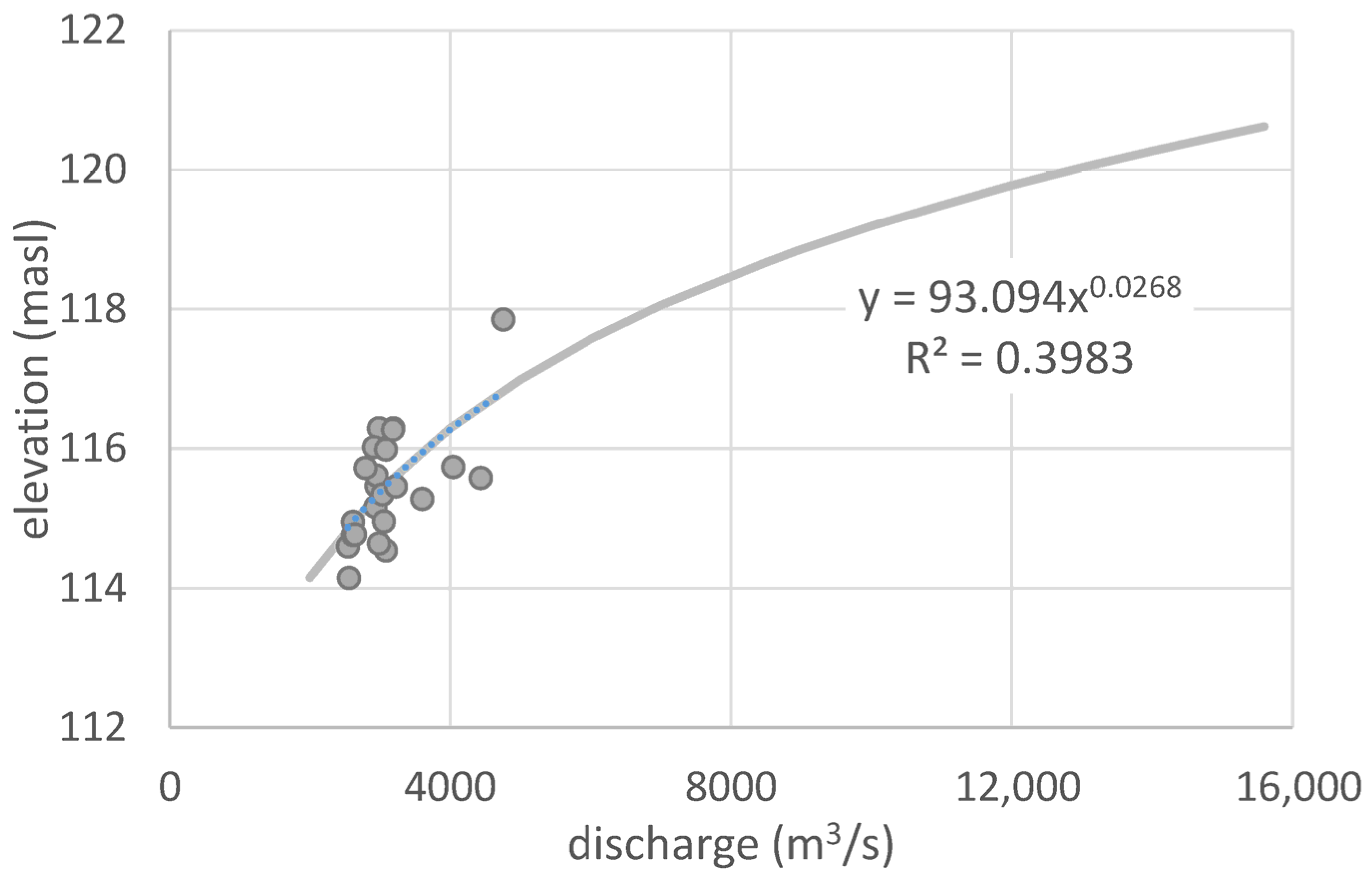
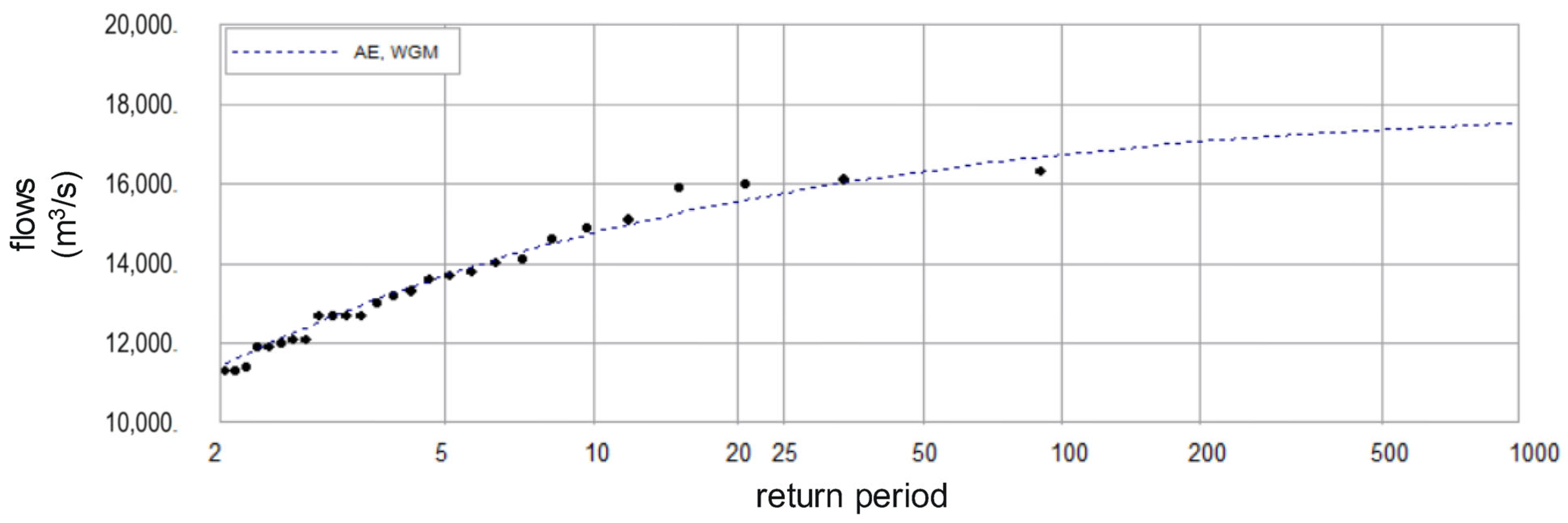
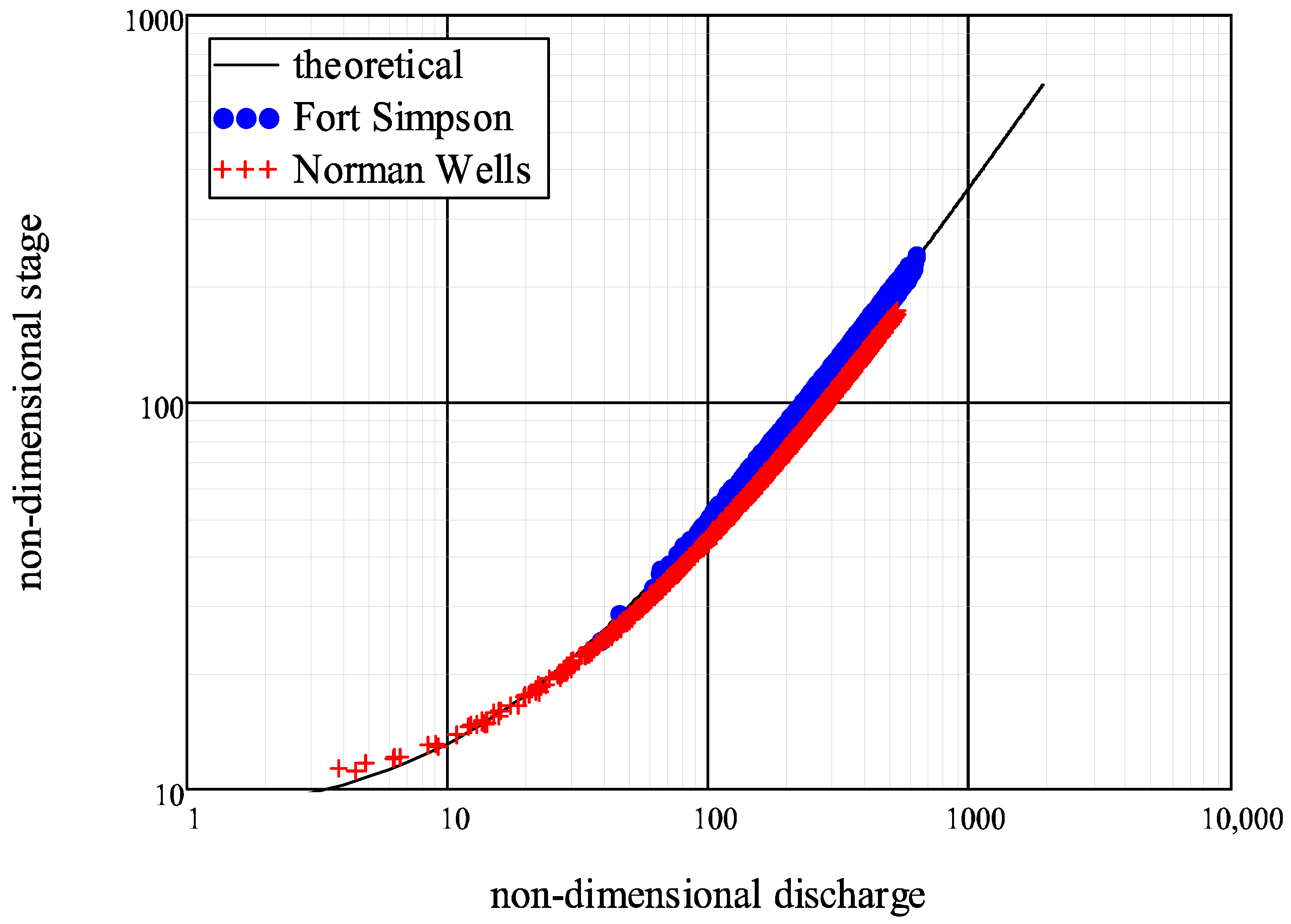
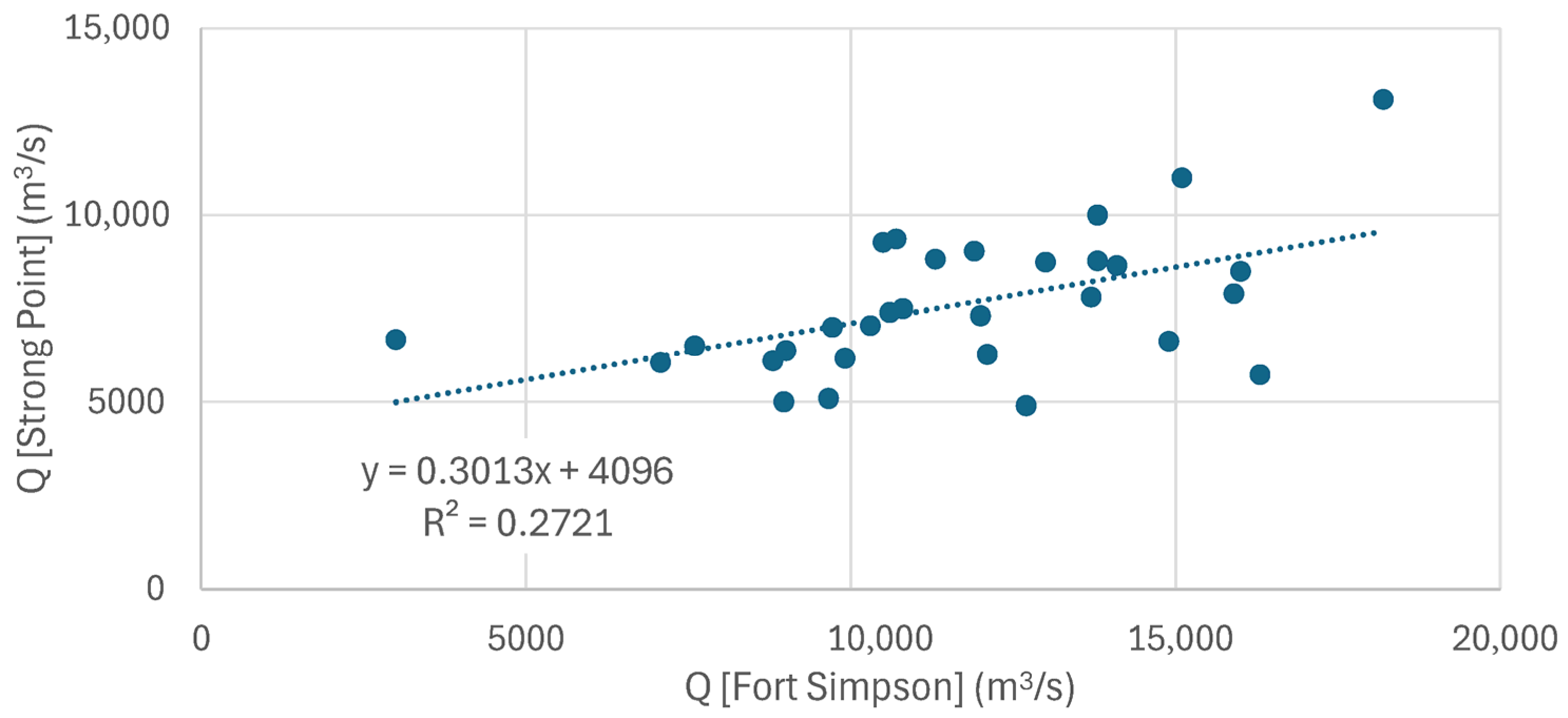
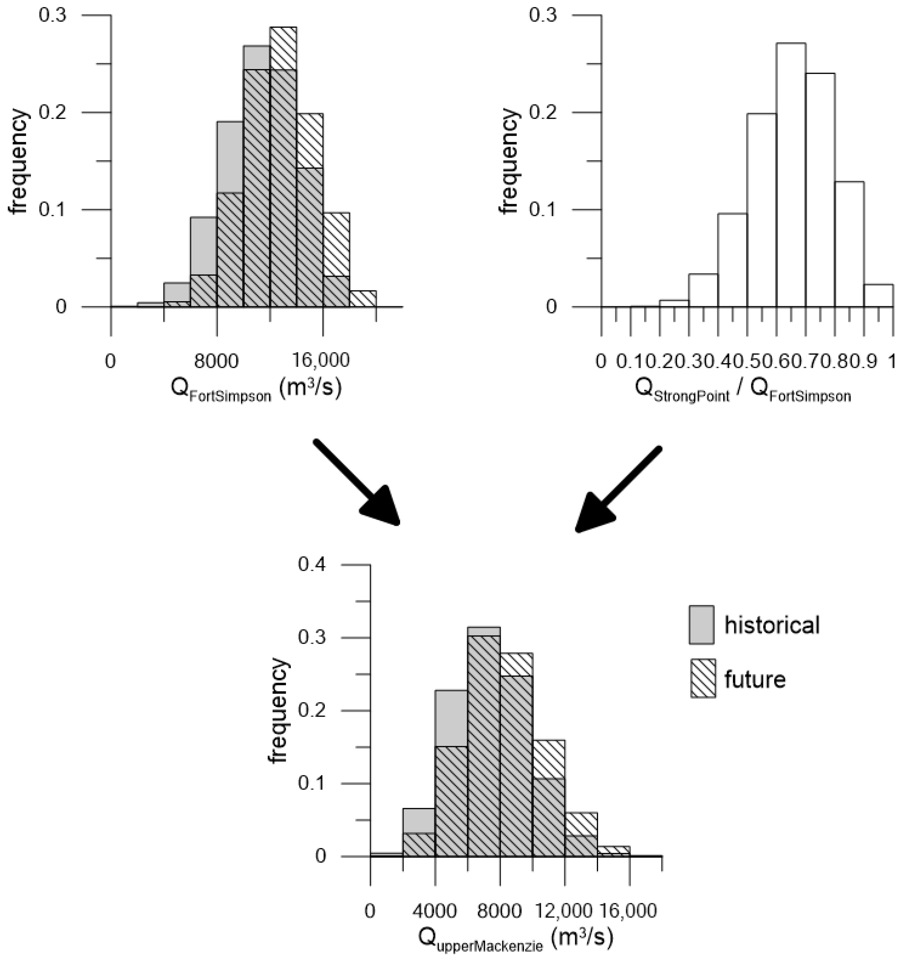
4.1.1. (i) Flow Frequency Curve

Flows at the end of the breakup period are necessary as input for the dimensionless discharge ξ in Equation (1). For the Monte-Carlo Analysis, it is essential to have a frequency distribution of these flows, which is illustrated in Figure 10, from which values can be randomly extracted. The generalized extreme value distribution was found to provide the best fit to the data.

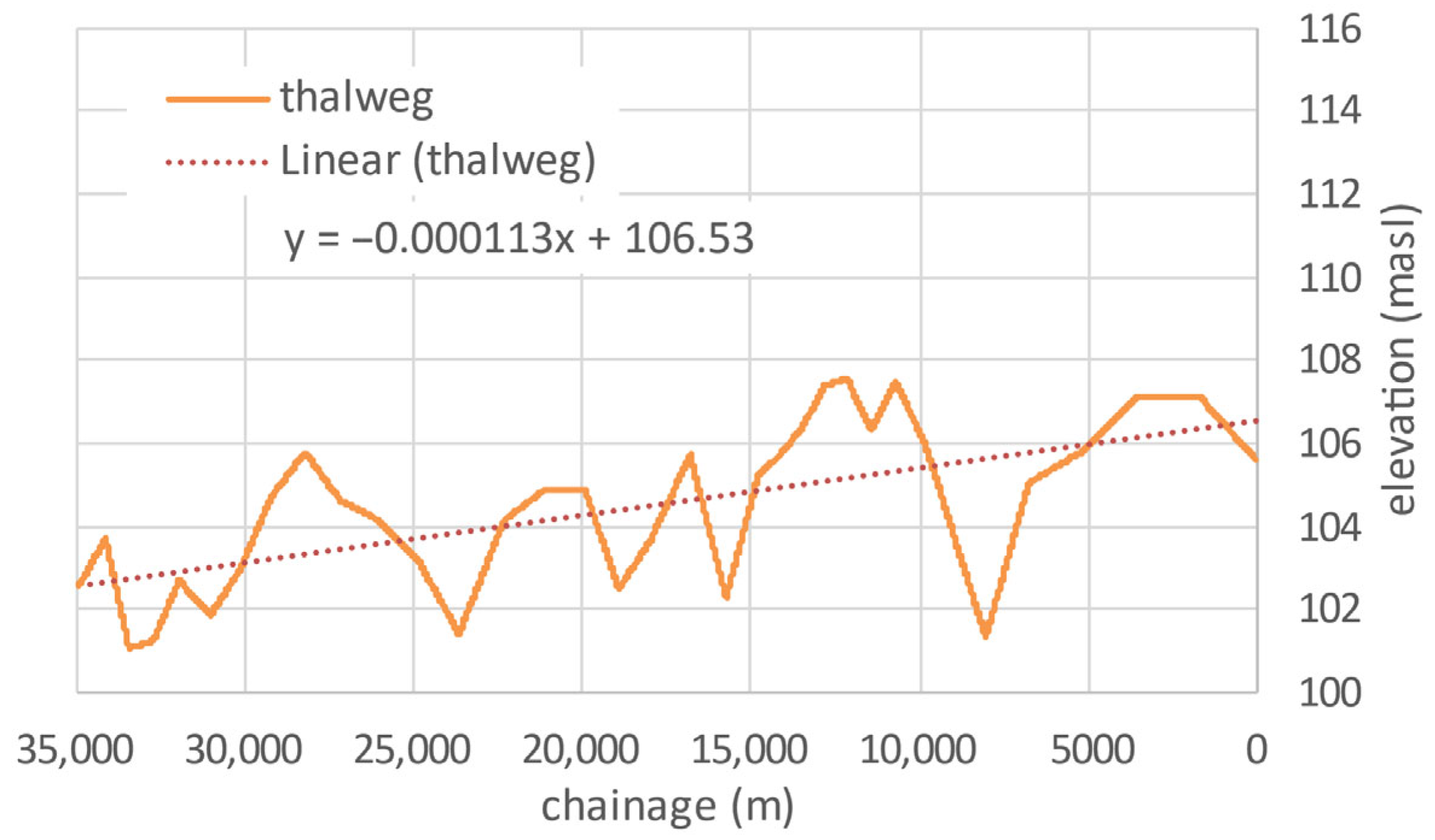
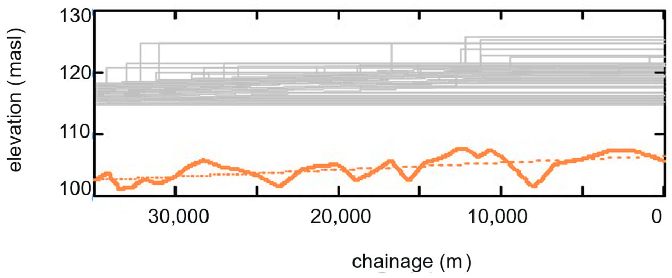
4.1.2. (ii) Slope from Thalweg

The thalweg was extracted from the bathymetric survey data and is indicated in Figure 11. A linear trendline was fit to the thalweg points to obtain a slope of 0.000113 for the reach.

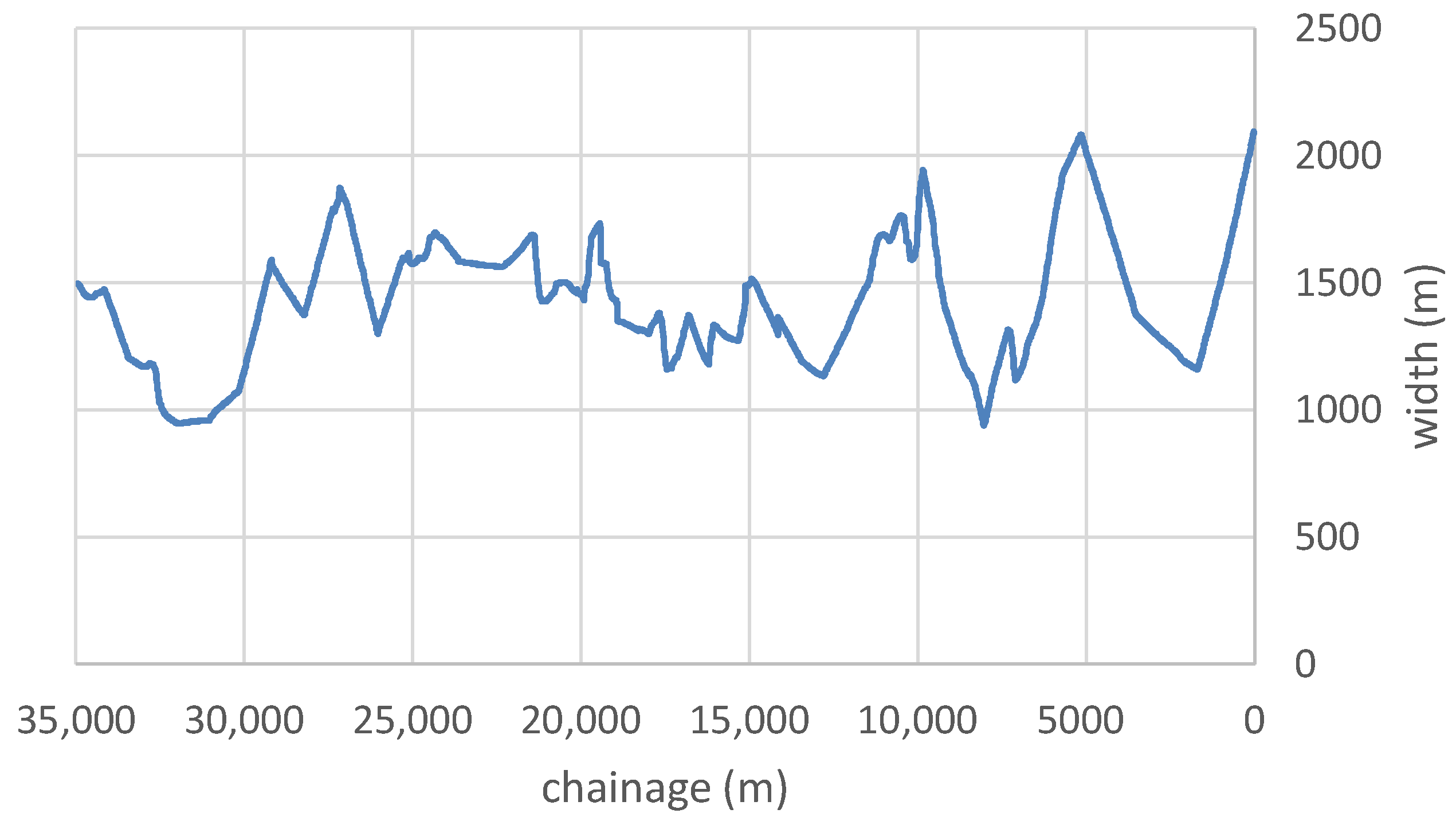
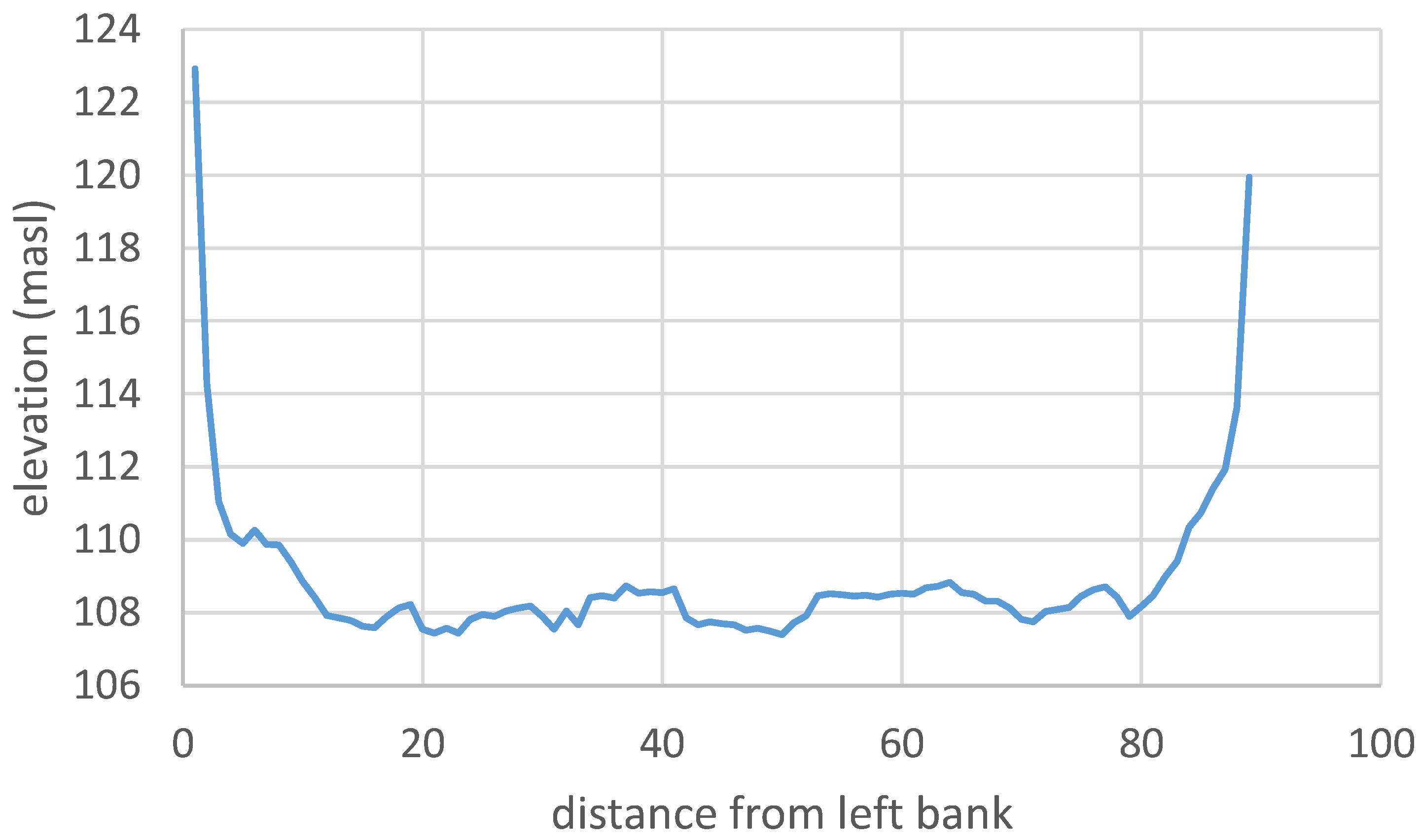
4.1.3. (iii) Widths Along Reach

The bathymetric survey consisted of 34 cross-sections along the Mackenzie River extending over a course of 34.9 km. River widths were extracted from each cross-section and interpolated into locations between the cross-sections. The variation in width along the chainage of the studied river reach is shown in Figure 12.

4.1.4. (iv to vi) Range of Parameters f_o, f_i/f_o and m:

The ranges of the calibration parameters were found to be:

-

composite friction parameter: 0.105 < f_o < 0.135

-

ratio ice friction to composite friction: 1.3 < f_i/f_o < 1.5

-

ice strength parameter: 1.4 < m < 1.6

The ranges in the non-dimensional discharge ξ and stage η are depicted alongside the theoretical η = f(ξ) in Figure 13. For comparison, the results for Norman Wells, situated more than 600 km downstream of Fort Simpson, are also included from another study [25]. The theoretical line provides a large range of non-dimensional discharge vs. stage values. The cluster of values calculated for Fort Simpson is higher than that of Norman Wells, due to fluvial geomorphological differences between the two sites. The Mackenzie River at Fort Simpson is narrower and more sloped than at Norman Wells potentially leading to a higher severity of ice jam floods at Fort Simpson.

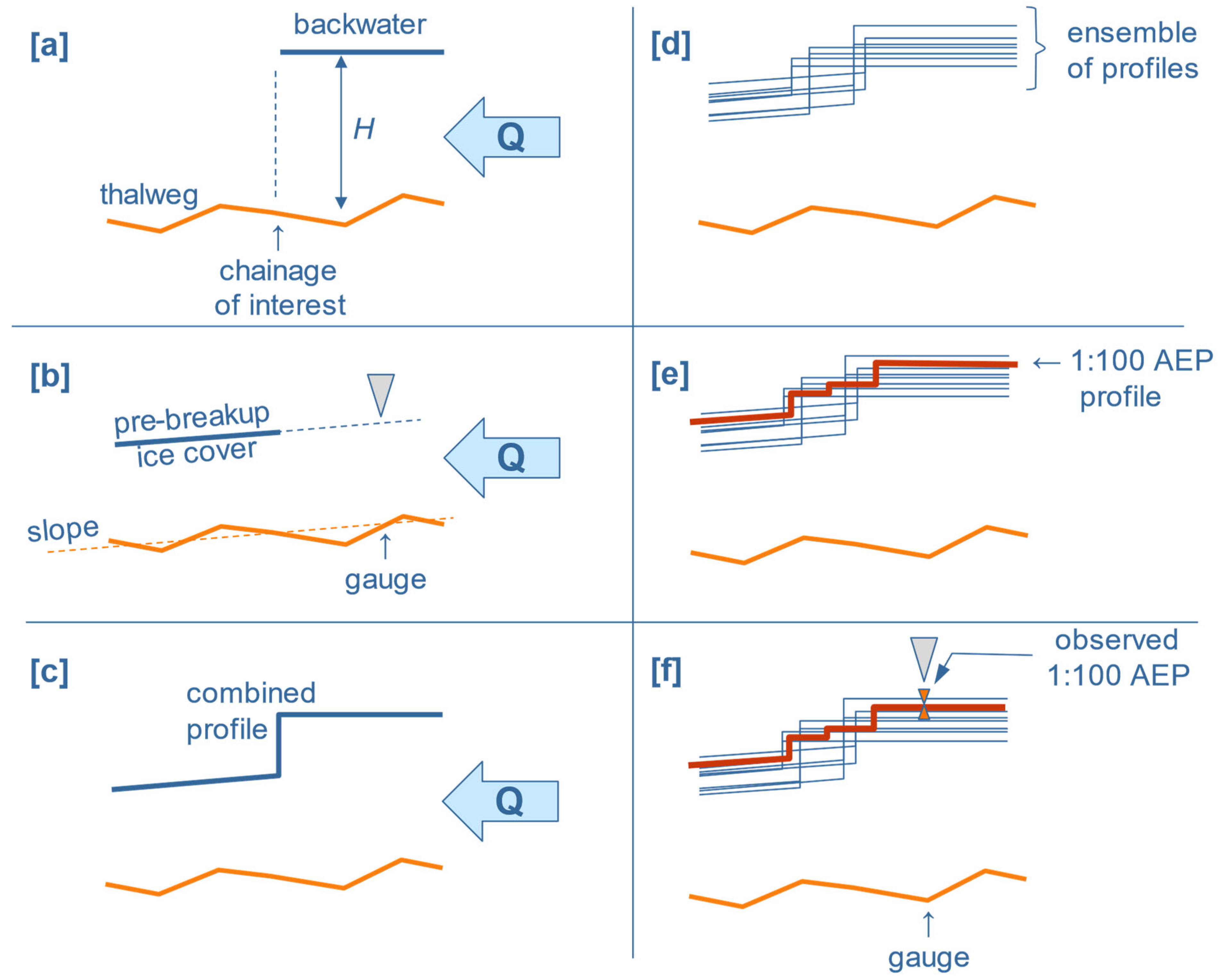
4.1.5. (vii and viii) Backwater Depth Calculations:

Equations (1) and (4) were set up in a Monte-Carlo framework in which ξ and η were calculated 10,000 times, with each calculation having a different set of parameters drawn randomly from distributions to yield 10,000 depth H values (Equation (3)) and maximum ice-jam thicknesses t values (Equation (6)).

To determine the geodetic elevations of the backwater levels, the values of H are added to the geodetic elevation of the thalweg. For example, the cross-section surveyed at the gauge located at Fort Simpson is illustrated in Figure 14.

4.1.6. (ix) Ensemble of Ice-Jam Profiles:

For a certain discharge and chainage location, an ice-jam profile consists of a

-

backwater level extending horizontally from the chainage location in the upstream direction, and

-

pre-breakup ice-cover water level extending from the same chainage location in the downstream direction with the same slope as the thalweg.

The trendline of the downstream portion of the profile (downstream of the ice-jam toe) should pass through the gauge at a level corresponding to the rating curve for pre-breakup under-ice flow, as shown in Figure 8. The observations stem from under-ice flow measurements carried out in the months of January, February, March and April in the years 2013 to 2022. The surveys were carried out by Water Survey of Canada using an ADCP; the data was shared with the Government of Northwest Territories in December 2023. Figure 15 gives an example of an ensemble of ice-jam profiles.

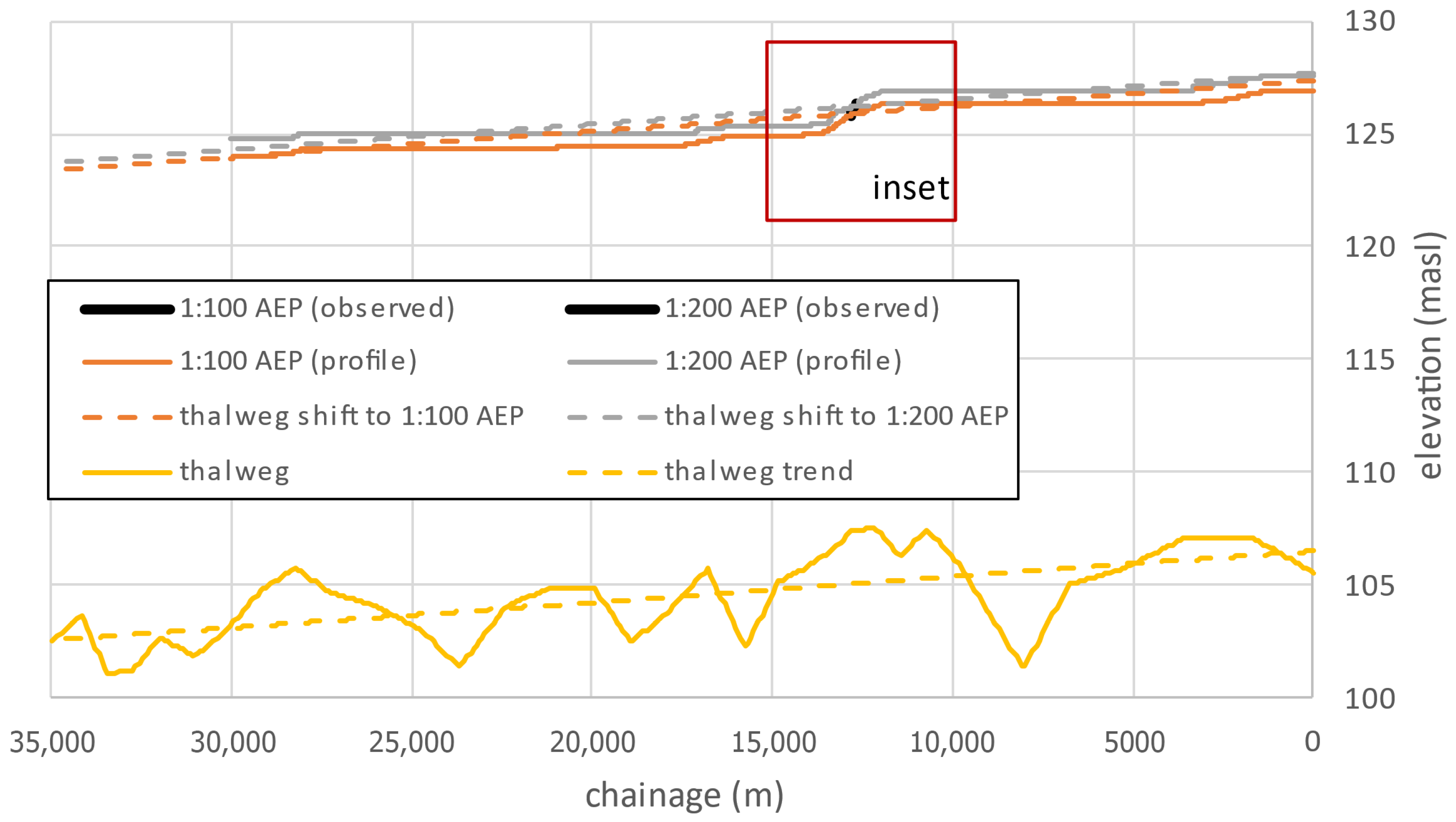
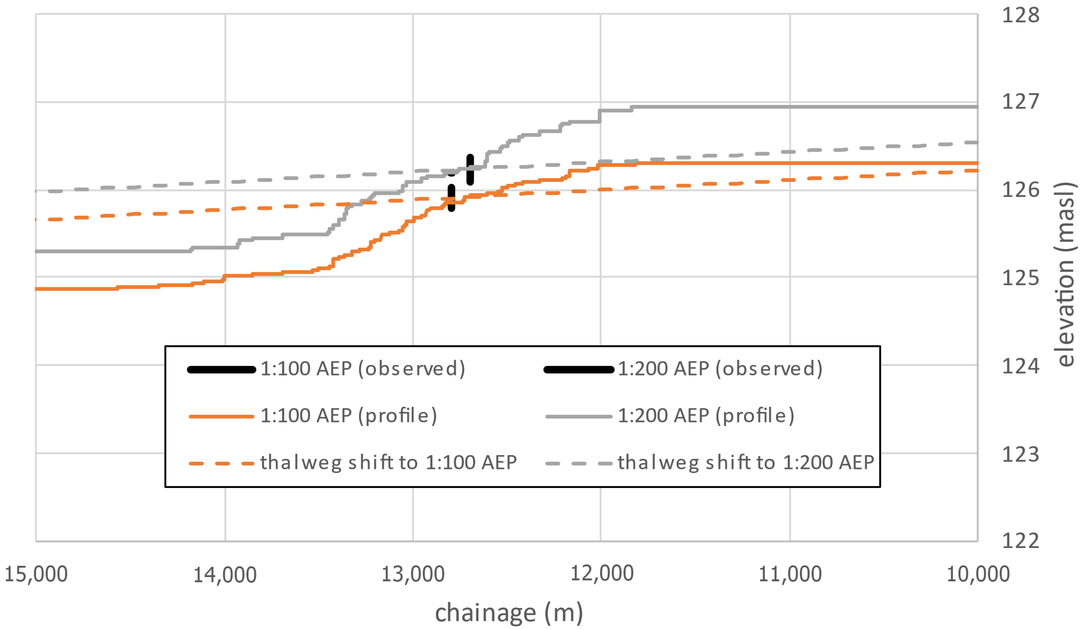
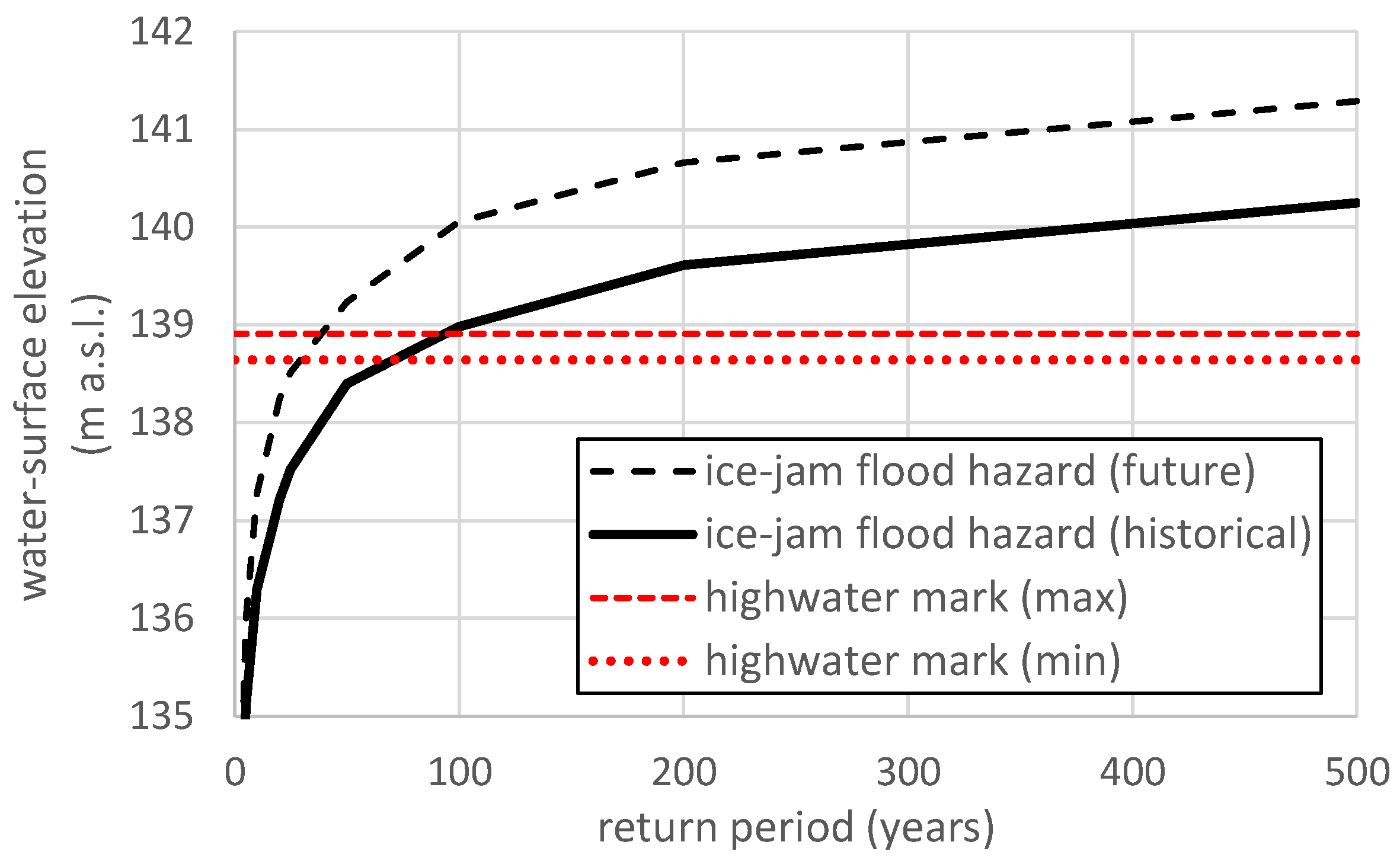
4.1.7. (x–xii) Return Periods of Backwater Level Profiles:

Percentiles that correspond to the 1:100 and 1:200 AEP were then extracted from all of the ice-jam profiles, as shown in Figure 16 (entire studied reach) and Figure 17 (zoomed in portion). The parameters f_o, f_i/f_o and μ were adjusted until the calculated stage frequency curve lay between the observed maximum and minimum stage frequency curves.

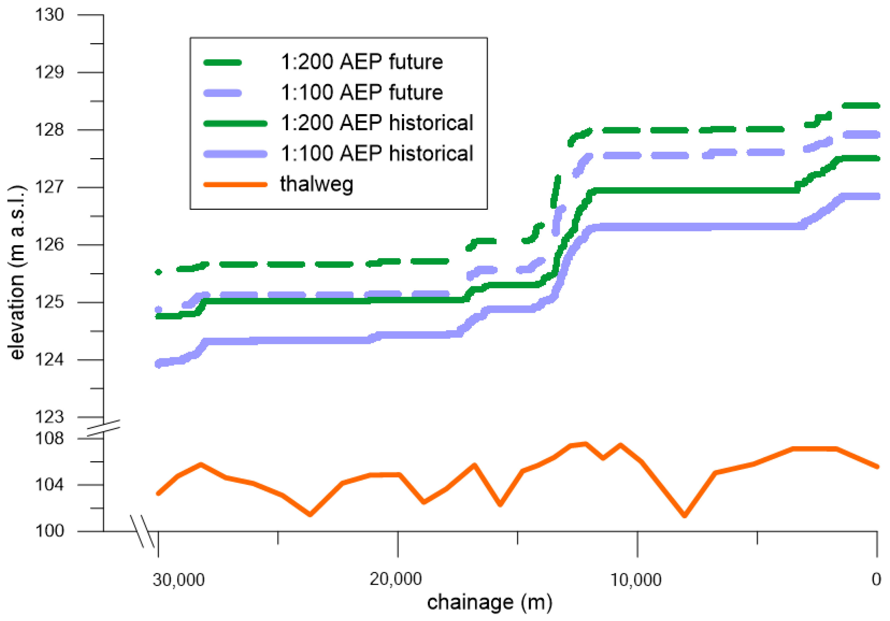
4.2. Shift in Ice-Jam Flood Hazard Assessment at Fort Simpson Due to Climate Change

Ice-jam flood hazard was compared between the status quo (historical: 1997–2021) and the impacts caused by climate change (future: 2076–2011). We are not accounting for changes in ice properties due to climate change, only changes in the climate and hydraulic regimes. The distribution of the status quo breakup flows was shifted for the future timeframe using the methodology presented in Dehghani Sanij et al. [16]. Figure 18 shows the shift to higher ice-jam flood hazard, indicated by the 1:100 and 1:200 AEP profiles, for the future 2076–2100 period, compared to the historical 1997–2021 period.

4.3. Reach-Based Extrapolation of Ice-Jam Flood Hazard to Ungauged Reach at Jean Marie River

The ice-jam flood hazard assessment was extrapolated to the ungauged reach of the Mackenzie River at the community of Jean Marie River upstream of Fort Simpson. The extrapolation was carried out similar to the methodology laid out in Lindenschmidt et al. [3]. One difference applied here was replacing the breakup flow distribution with a distribution of the fraction of the breakup flows recorded at Strong Point to those recorded at Fort Simpson. The flow at Fort Simpson is constituted by both the flows from the Liard River, which flows into the Mackenzie River just upstream of Fort Simpson, and the (upper) Mackenzie River flows upstream of the Liard River mouth. At breakup, the upper Mackenzie River contributed, on average, approximately 65% (a fraction of 0.65) of the flows at Fort Simpson, with the distribution shown in Figure 19. The remaining flows stem from the Liard River. The correlation between the two flows at breakup is low (r² = 0.27), as indicated in Figure 19. This is due to the differing ice regimes from year-to-year at the Mackenzie/Liard River confluence. Lindenschmidt [17] compared the breakup end dates at Strong Point with those at Fort Simpson and determined that the breakup does not always occur earlier at Strong Point than at Fort Simpson itself. In some years, ice sheets and accumulations still persist upstream of the confluence even though the ice cover at Fort Simpson has broken up. The b-flag analysis was also carried out for flow records of the Liard River near its mouth. By comparing 45 years (1973–2017) of breakup end dates recorded at the gauges at Fort Simpson and the Liard River mouth, it was found that for 5 years out of the 45-year series the ice cover in the vicinity of the mouth of the Liard River persisted longer than the ice cover at Fort Simpson.

The frequency distribution of the flow fractions in Figure 20 was fit with a GEV distribution shown in Figure 21. Randomly selecting a flow fraction and multiplying it to a randomly selected Fort Simpson flow provided a random flow at Jean Marie River. The parameterization of the ice properties calibrated at Fort Simpson were transferred to the Jean Marie River calculations. The fluvial geomorphological parameters width and slope were adjusted to the setting at Jean Marie River. Using Manning’s equation, the thalweg elevation at Jean Marie River was back calculated from the sites’ average slopes, widths and flows. The resulting status quo (historical) ice-jam flood hazard curve for Jean Marie River is shown in Figure 22.

4.4. Shift in Ice-Jam Flood Hazard Assessment at Jean Marie River Due to Climate Change

To determine the impacts of climate change on the flow distribution, the status quo flow distribution used for the Jean Marie River ice-jam flood hazard assessment was replaced with a projected flow distribution of the future (2076–2100) period. The same flow fraction distribution was used on the future breakup flow distribution for Fort Simpson to determine the future flow distribution at Jean Marie River. The future ice-jam flood hazard assessment is superimposed with the historical assessment in Figure 22, showing an expected increase in the ice-jam flood hazard in the future. This assessment corresponds to the ice-jam flood hazard at a point adjacent to Jean Marie River’s community center. Longitudinal profiles of the 1:100 and 1:200 AEP were extended upstream and downstream along the river from this point, respectively, increased and decreased by an amount that remained true to the slope of the reach.

5. Conclusions

5.1. Ice-Jam Flood Hazard Assessment

A detailed analysis of the ice-jam flood hazard along the river reach at Fort Simpson was successfully attained. The generalized extreme value distribution was found to best fit the flow data at the end of the breakup period, which is crucial for the Monte-Carlo Analysis. The slope of the thalweg, derived from bathymetric survey data, is 0.000113. Varying the composite friction parameter, ice friction to composite friction ratio, and ice strength parameter within a Monte-Carlo framework, along with randomizing ice-jam discharges and toe locations, yielded ensembles of backwater level profiles from which profiles of the 1:100 and 1:200 annual exceedance probabilities (AEPs) were extracted. Parameters were adjusted to match observed stage frequency curves.

5.2. Reach-Based Extrapolation and Climate Change

The ice-jam flood hazard assessment was also successfully extrapolated from the gauged (Fort Simpson) to the ungauged (Jean Marie River) reach. Changes in the 1:100 and 1:200 AEP flood depths due to climate impacts were also ascertained for both sites, with flooding becoming more severe by the end of this century.

5.3. Addressing Uncertainties Using the Monte-Carlo Analysis Framework

The Monte-Carlo analysis provides a framework to account for uncertainty in the ice-jam hazard assessment by simulating a wide range of possible ice-jam scenarios. This approach involves generating numerous simulations with varying input parameters to reflect the inherent variability and unpredictability of ice-jam events. By doing so, it creates an ensemble of potential outcomes, each representing different conditions and responses of the river system to ice jams. For instance, the framework can simulate different combinations of water flow rates and ice roughness parameters to capture the range of possible water surface elevations and flood extents that could result from ice jams. The results are then used to create probability profiles, such as non-exceedance probability profiles, which indicate the likelihood of different flood levels occurring. Hence, this method allows for a more comprehensive understanding of the potential flood hazards by considering the full spectrum of possible scenarios, rather than relying on a single deterministic model. It helps to identify the most likely outcomes and the range of uncertainties, providing a more robust basis for flood risk management and decision-making.

5.4. Suggestions for Future Work

This study applied an empirical relationship between flows and ice-jam backwater levels to produce longitudinal profiles of ice-jam flood hazard along the river. Another method suggested by Turcotte and Saal [26] may use the slope of the energy profile for open-water flows as the ice-jam flood hazard profile if the thalweg slope remains constant along the reach. A third method is also an ensemble method but embeds a numerical river-ice hydraulic model, such as RIVICE, in the Monte-Carlo framework instead of the empirical equations. This would allow more ice-jam processes to be simulated with greater flexibility and accuracy. A comparison of these three methods, and potentially others, could be cataloged in a guideline allowing river engineers and flood managers to tailor their ice-jam flood hazard assessment exercises accordingly to the complexity of the study site and data availability.

The Monte-Carlo framework provides an avenue to investigate the impact of scenarios representing changes in fluvial geomorphological and ice regimes. For instance, in this study, slope was assumed to remain constant throughout the reaches (see [ii] in conceptualization shown in Figure 6), however other sites do have varying slopes along the reach, such as the studied reach at Fort McMurray along the Athabasca River [2] requiring the distribution to vary along the reach (see [A] in modified conceptualization in Figure 23). Also, the propensity of ice-jam lodgment may vary along the reach requiring a more stepped distribution of the ice-jam toe location (see [B] in modified conceptualization in Figure 23). Mitigation options can also be tested for ice-jam flood hazard reduction, for instance, constraining the ice-jam toe distribution (see [C] in modified conceptualization in Figure 23) to mimic artificial pre-breakage of the ice cover to prevent ice-jam lodgments in those river sections during natural spring breakup [2].

References

1. Lindenschmidt, K.-E.; Sydor, M.; van der Sanden, J.; Blais, E.; Carson, R.W. Monitoring and modeling ice cover formation on highly flooded and hydraulically altered lake-river systems. In Proceedings of the 17th CRIPE Workshop on the Hydraulics of Ice Covered Rivers, Edmonton, AB, Canada, 21–24 July 2013; pp. 180–201. Available online: http://cripe.ca/docs/proceedings/17/Lindenschmidt-et-al-2013.pdf (accessed on 21 July 2025).
2. Lindenschmidt, K.-E. River Ice Processes and Ice Flood Forecasting—A Guide for Practitioners and Students, 2nd ed.; Springer Nature Switzerland AG: Cham, Switzerland, 2024. [Google Scholar] [CrossRef]
3. Lindenschmidt, K.-E.; Coles, A.; Saade, J. Reach-based extrapolation to assess the ice-jam flood hazard of an ungauged river reach along the Mackenzie River, Canada. Water 2024, 16, 1535. [Google Scholar] [CrossRef]
4. Rokaya, P.; Budhathoki, S.; Lindenschmidt, K.-E. Trends in the Timing and Magnitude of Ice-Jam Floods in Canada. Sci. Rep. 2018, 8, 5834. [Google Scholar] [CrossRef] [PubMed]
5. Turcotte, B.; Morse, B.; Pelchat, G. Impact of Climate Change on the Frequency of Dynamic Breakup Events and on the Risk of Ice-Jam Floods in Quebec, Canada. Water 2020, 12, 2891. [Google Scholar] [CrossRef]
6. Simonovic, S.P.; Li, L. Methodology for Assessment of Climate Change Impacts on Large-Scale Flood Protection System. J. Water Resour. Plan. Manag. 2003, 129, 361. [Google Scholar] [CrossRef]
7. Turcotte, B.; Burrell, B.; Beltaos, S. The Impact of Climate Change on Breakup Ice Jams in Canada: State of knowledge and research approaches. CGU HS Committee on River Ice Processes and the Environment. In Proceedings of the 20th Workshop on the Hydraulics of Ice Covered Rivers, Ottawa, ON, Canada, 14–16 May 2019; Available online: https://cripe.ca/docs/turcotte-et-al-2019-pdf (accessed on 21 July 2025).
8. Prowse, T.; Alfredsen, K.; Beltaos, S.; Bonsal, B.; Duguay, C.; Korhola, A.; McNamara, J.; Pienitz, R.; Vincent, W.F.; Vuglinsky, V.; et al. Past and future changes in Arctic lake and river ice. Ambio 2011, 40, 53–62. [Google Scholar] [CrossRef]
9. Andrishak, R.; Hicks, F. Simulating the effects of climate change on the ice regime of the Peace River. Can. J. Civ. Eng. 2008, 35, 461–472. [Google Scholar] [CrossRef]
10. Das, A.; Rokaya, P.; Lindenschmidt, K.-E. Ice-jam flood risk assessment and hazard mapping under future climate. J. Water Resour. Plan. Manag. 2020, 146, 04020029. [Google Scholar] [CrossRef]
11. Rokaya, P.; Morales, L.; Bonsal, B.; Wheater, H.; Lindenschmidt, K.-E. Climatic effects on ice phenology and ice-jam flooding of the Athabasca River in western Canada. Hydrol. Sci. J. 2019, 64, 1265–1278. [Google Scholar] [CrossRef]
12. Peters, D.L.; Monk, W.A.; Baird, D.J. Cold-regions hydrological indicators of change (CHIC) for ecological flow needs assessment. Hydrol. Sci. J. 2014, 59, 502–516. [Google Scholar] [CrossRef]
13. Shrestha, R.; Schnorbus, M.A.; Peters, D.L. Assessment of a hydrologic model’s reliability in simulating flow regime alterations in a changing climate. Hydrol. Process. 2016, 30, 2628–2643. [Google Scholar] [CrossRef]
14. Beltaos, S. River ice jams: Theory, case studies and application. J. Hydraul. Eng. 1983, 109, 1338–1359. [Google Scholar] [CrossRef]
15. Beltaos, S. River Ice Jams; Water Resources Publications, LLC.: Highlands Ranch, CO, USA, 1995. [Google Scholar]
16. Dehghani Sanij, M.; Lindenschmidt, K.-E.; Elshamy, M. Shifts in ice-jam flood hazard due to climate change along the Mackenzie River. Can. Water Resour. J. 2025; submitted. [Google Scholar]
17. Lindenschmidt (2021) Rapid assessment of ice-jam flooding at Fort Simpson along the Mackenzie River in the Northwest Territories. Report submitted by Karl-Erich Lindenschmidt to Wood in June 2021, which was integrated into a larger report for the Government of Northwest Territories.
18. Andrishak, R.; Van Der Vinne, G. Climate and ice impacts on Great Slave Lake levels and flows in the Mackenzie River, Northwest Territories CGU HS Committee on River Ice Processes and the Environment. In Proceedings of the 19th Workshop on the Hydraulics of Ice Covered Rivers, Whitehorse, YT, Canada, 9–12 July 2017; Available online: http://cripe.ca/docs/proceedings/19/Andrishak-VanDerVinne-2017.pdf (accessed on 21 July 2025).
19. Hicks, F.E.; Chen, X.; Andres, D. Effects of Ice on the Hydraulics of the Mackenzie River at the Outlet of Great Slave Lake, NWT: A Case Study. Can. J. Civ. Eng. 1995, 22, 43–54. Available online: https://cdnsciencepub.com/doi/10.1139/l95-005 (accessed on 21 July 2025). [CrossRef]
20. Beltaos, S. River Ice Formation; Committee on River Ice Processes and the Environment, Canadian Geophysical Union: Edmonton, AB, Canada, 2023; ISBN 978-0-9920022-0-6. [Google Scholar]
21. White, K.D. Hydraulic and Physical Properties Affecting Ice Jams (Report 99–11). US Army Corps of Engineers’ Cold Regions Research and Engineering Laboratory. 1999. Available online: https://apps.dtic.mil/sti/tr/pdf/ADA375289.pdf (accessed on 21 July 2025).
22. Elshamy, M.E.; Pomeroy, J.; Pietroniro, A.; Wheater, H.; Abdelhamed, M.; Davison, B. Land Surface Hydrological Modelling of the Mackenzie River Basin: Parametrization to Simulate Streamflow and Permafrost Dynamics. J. Hydrol. 2025, 659, 133134. [Google Scholar] [CrossRef]
23. Elshamy, M.E.; Pomeroy, J.W.; Pietroniro, A.; Wheater, H.; Abdelhamed, M.S. The impact of climate and land cover change on the cryosphere and hydrology of the Mackenzie River Basin, Canada. Water Resour. Res. 2024, 1–49. [Google Scholar] [CrossRef]
24. Janowicz, J.R. Impacts of Climate Warming on River Ice Break-up and Snowmelt Freshet. Processes on the Porcupine River in Northern Yukon. In Proceedings of the 19th CRIPE Workshop on the Hydraulics of Ice Covered Rivers, Whitehorse, YT, Canada, 9–12 July 2017; Available online: https://cripe.ca/docs/nafziger-et-al-2021-pdf?wpdmdl=1404&refresh=66edfd55b9b1a1726872917 (accessed on 21 July 2025).
25. WSP (2025) Fort Good Hope flood inundation and hazard mapping study (Phase 1). Hydrology and hydraulics report submitted by WSP Canada Inc. to the Government of Northwest Territories.
26. Turcotte, B.; Saal, S. Flooding in Dawson: Exposure Analysis and Risk Reduction Recommendations. Presented to the Infrastructure Branch of the Department of Community Services, Government of Yukon. Yukon University Research Centre, Yukon. 2022, p. 90. Available online: https://www.yukonu.ca/sites/default/files/inline-files/Final_report_flooding_Dawson_CS-YRC.pdf (accessed on 21 July 2025).
Figure 1. Mackenzie River from Great Slave Lake to Jean Marie River and Fort Simpson (map: Google Earth).
Water 17 02288 g001
Figure 2. Beginning of freeze-up dates (first b-flag) and end-of-breakup dates (last b-flag) of the ice cover at Fort Simpson (gauge ID 10GC001).
Water 17 02288 g002
Figure 3. Sentinel-1 imagery showing the progression of the ice cover immediately before and also after the ice-jam flood peak (reached on 14 May 2021) at Fort Simpson (from [17]).
Water 17 02288 g003aWater 17 02288 g003b
Figure 4. Ice jam of thickness t along a river reach of slope S and width W for a discharge Q with backwater staging depth H and flow under the ice jam of depth h.
Water 17 02288 g004
Figure 5. Relationship between non-dimensional discharge ξ and non-dimensional ice-jam stage η for equilibrium ice jams [20].
Water 17 02288 g005
Figure 6. Conceptualization of the Monte-Carlo framework for the longitudinal profiles of ice-jam flood hazard.
Water 17 02288 g006
Figure 7. Construction of ensemble of ice-jam profiles to derive an ice-jam flood hazard profile: [a] backwater elevation extended upstream, [b] downstream profile follows thalweg slope, [c] combining upstream and downstream profiles at each chainage, [d] creation of ensemble of profiles, [e] estimate return period/probability of every flood profile and [f] comparison with observed AEP level at the gauge.
Water 17 02288 g007
Figure 8. Under-ice rating curve derived from ADCP under-ice flow measurements carried out at Fort Simpson.
Water 17 02288 g008
Figure 9. Log-normal distribution fit to observed cumulative degree days of melting, beginning 1 April, until breakup for the years 1965 to 2021.
Water 17 02288 g009
Figure 10. Frequency distributions of flows recorded at the end of spring breakup (flow with last recorded b-flag) at Fort Simpson.
Water 17 02288 g010
Figure 11. Thalweg along the reach at Fort Simpson, from which slope was calculated upstream to downstream (right to left).
Water 17 02288 g011
Figure 12. Widths along the Fort Simpson reach extracted from the bathymetric survey (upstream to downstream looking right to left).
Water 17 02288 g012
Figure 13. Ranges of non-dimensional discharge ξ and non-dimensional ice-jam stage η for equilibrium ice jams at Fort Simpson and Norman Wells.
Water 17 02288 g013
Figure 14. Cross-section at the Fort Simpson gauge (provided by Government of Northwest Territories).
Water 17 02288 g014
Figure 15. Ensemble of ice-jam profiles; only a subset of the ensemble is shown for clarity. The gauge is located at chainage 12,800 m.
Water 17 02288 g015
Figure 16. Profiles of 1:100 and 1:200 AEP for the reach at Fort Simpson; a zoom into the inset is provided in the next figure.
Water 17 02288 g016
Figure 17. Zoomed in from the previous figure, the 1:100 AEP and 1:200 AEP profiles at Fort Simpson. Observed 1:100 AEP and 1:200 AEP represent the best three fits for the calculated water surface elevation from the observed gauge data.
Water 17 02288 g017
Figure 18. Longitudinal profiles of the 1:100 and 1:200 AEP ice-jam flood hazard along Fort Simpson, for the historical and future time frames.
Water 17 02288 g018
Figure 19. Fraction of flow at Strong Point compared to the flow at Fort Simpson.
Water 17 02288 g019
Figure 20. Low correlation between breakup flows along the Mackenzie River immediately downstream (at Fort Simpsons) and upstream (at Strong Point) of the Liard River confluence.
Water 17 02288 g020
Figure 21. Distributions of flows at Fort Simpson (upper left) and the upper Mackenzie River (bottom) using the flow faction distribution (upper right); all distributions stem from values generated randomly from GEV distributions.
Water 17 02288 g021
Figure 22. Ice-jam flood hazard at Jean Marie River for the historical and future timeframes.
Water 17 02288 g022
Figure 23. Adjustments to the distributions to accommodate changes in [A] bed slope along the reach, [B] varying propensity to ice-jam lodgments along the reach and [C] mitigation measures to remove ice-jam lodgments in certain sections of the reach.
Water 17 02288 g023