Present and Future Energy Potential of Run-of-River Hydropower in Mainland Southeast Asia: Balancing Climate Change and Environmental Sustainability

Abstract

Southeast Asia relies heavily on hydropower from dams and reservoir projects, but this dependence comes at the cost of ecological damage and increased vulnerability to extreme events. This dilemma necessitates a choice between continued dam development and adopting alternative renewable options. Concerns over these environmental impacts have already led to halts in dam construction across the region. This study assesses the potential of run-of-river hydropower plants (RHPs) across 199 hydrometric stations in Mainland Southeast Asia (MSEA). The assessment utilizes power duration curves for the historical period and projections from the HBV hydrological model, which is driven by an ensemble of 31 climate models for future scenarios. Energy production was analyzed at four levels (minimum, maximum, balanced, and optimal) for both historical and future periods under varying Shared Socioeconomic Pathways (SSPs). To promote sustainable development, environmental flow constraints and carbon dioxide (CO₂) emissions were evaluated for both historical and projected periods. The results indicate that the aggregate energy production potential during the historical period ranges from 111.15 to 229.62 MW (Malaysia), 582.78 to 3615.36 MW (Myanmar), 555.47 to 3142.46 MW (Thailand), 1067.05 to 6401.25 MW (Laos), 28.07 to 189.77 MW (Vietnam), and 566.13 to 2803.75 MW (Cambodia). The impact of climate change on power production varies significantly across countries, depending on the level and scenarios. At the optimal level, an average production change of −9.2–5.9% is projected for the near future, increasing to 15.3–19% in the far future. Additionally, RHP development in MSEA is estimated to avoid 32.5 Mt of CO₂ emissions at the optimal level. The analysis further shows avoidance change of 8.3–25.3% and −8.6–25.3% under SSP245 and SSP585, respectively.

1. Introduction

Despite the targets set by the groundbreaking Paris Agreement to address global climate challenges, carbon dioxide (CO₂) emissions have continued to rise, reaching a peak of 37.4 Gt in 2023, as reported by the International Energy Agency [1]. The United Nations aims to reduce global CO₂ emissions by 45% by 2030 and achieve net-zero emissions by 2050 [2], underscoring the need for an energy transformation. The world’s heavy reliance on fossil fuels, which supply around 80% of global energy needs, highlights the urgent necessity for a swift transition to clean energy solutions aligned with development goals and environmental priorities [3,4]. Expanding renewable energy sources, such as hydropower, is a key strategy for reducing emissions, particularly in regions with abundant water resources, where it can contribute to clean energy generation and sustainable growth. However, the effectiveness of hydropower varies significantly due to geographic and temporal factors. As noted by Jakimavičius et al. [5], the long-term viability of hydropower is influenced by multiple factors, including financial considerations, geographical location, regulatory frameworks, and environmental constraints. A critical challenge in this context is understanding how future climate change will impact hydropower production and CO₂ emissions. Ultimately, developing a robust assessment of hydropower potential requires a comprehensive evaluation of environmental consequences and evolving climate conditions on a global scale.

Over the past few decades, Southeast Asia (SEA) has actively pursued economic growth and deeper integration into the global economy. This progress has driven increases in economic activity and population. However, a major challenge accompanying this development is the growing imbalance between energy supply and demand. As a result, the region remains heavily reliant on fossil fuels and thermal power generation, leading to a surge in CO₂ emissions and significant environmental impacts [6]. In 2020, for instance, SEA contributed 1.6 Gt of greenhouse gas emissions to the global total [7]. The rising environmental costs pose a challenge to the region’s future economic growth. Many studies highlight the potential of SEA’s abundant renewable energy sources, particularly hydropower, as a viable solution to energy shortages and environmental concerns [6,8]. Run-of-river hydropower plants (RHPs) are considered an efficient means of energy generation, as they harness the natural flow of rivers rather than relying on large dams and water storage, as seen in reservoir-based power plants [9]. However, RHPs are highly sensitive to seasonal variations in river flow [10]. Extensive research has been conducted to evaluate the benefits and impacts of hydropower plants across various regions worldwide; with studies focusing on locations such as Brazil [11,12], Switzerland [13], the European Union [14], the USA [15], the Amazon Basin [16], China [17], and Lithuania [5], among others.

In the context of SEA, there are also several studies concerning hydropower energy. Arias et al. [18] investigated the effects of the Mekong River’s hydropower development and climate change on Tonle Sap Lake in SEA. A reduction in seasonal water fluctuation of 0.33 ± 0.25 m was the combined effect of hydropower development and climate change on the lake. Aroonrat, Wongwises [19] assessed Thailand’s current hydropower potential in a similar study. The results showed an efficiency of 11% of Thailand’s total hydropower potential. The study identified 25 riverine areas in Thailand for small-scale hydropower. Purwanto, Afifah [20] evaluated the impact of techno-socioeconomic factors on the sustainability of the Rimba Lestari and Mendolo micro-hydropower projects in Indonesia. Despite the project’s social success, the results showed the economic weakness of both power plants. Yah et al. [21] identified Malaysia’s small-scale hydropower potential for rural electrification in 2017. The study discovered that Malaysia has only utilized 17.5% of its 500 MW small-scale hydropower potential. Although hydropower is a significant option in Malaysia, its utilization has been limited due to economic and institutional constraints. Tang et al. [6] assessed the hydropower status of Thailand, Malaysia, Indonesia, and Myanmar from 2005 to 2015. The results showed that these countries have abundant hydropower resources available, and the governments of Malaysia, Indonesia, and Thailand are pursuing hydropower development. On the other hand, the Myanmar government’s policies on hydropower development are quite weak. This study suggested the development of small-scale hydropower in Thailand, Indonesia, and Malaysia. Siala et al. [22] examined solar energy as an alternative to large hydropower projects. The study found that costs would only increase by 2.4% from 2016 to 2037, assuming a scenario where all dam construction in the Lower Mekong was stopped. Another study investigated energy consumption and CO₂ emissions from fossil and renewable energy sources in SEA [7]. The results showed a scattered distribution of renewable resources and low to moderate changes. The results also highlighted that despite renewable energy providing 20% of total energy consumption in 2015, the current rate of these energies is far from the goal of net-zero CO₂ emissions by 2050. Sakti et al. [8] developed a spatial model for the potential of renewable energy in Southeast Asia, including solar, wind, and hydropower in residential and agricultural areas. The results identified high and low potential for renewable energy production in northern SEA and areas close to the equator (excluding southern regions).

Based on the literature review, several research gaps have been identified. Firstly, there is an overreliance on large dams and an underestimation of the potential of RHPs. Hydropower, the primary source of electricity in Vietnam, Laos, Myanmar, and Cambodia, depends heavily on large dams along the Mekong River and its tributaries. However, uncontrolled dam construction has resulted in significant ecological and environmental damage as well as increased vulnerability to extreme events [23]. These concerns have led to the suspension of dam construction in some areas, such as Cambodia [24]. While alternative renewable energy sources like solar and wind power are inefficient in the region [7], the potential of RHPs has been largely overlooked, highlighting the need for a reassessment of hydropower diversification strategies. Secondly, existing studies often fail to integrate CO₂ emission assessments with future hydropower production projections. A more comprehensive analysis is required to evaluate the environmental benefits of different hydropower options and their role in reducing carbon emissions under future climate scenarios. Lastly, general circulation models (GCMs) introduce uncertainties in climate projections, and existing studies do not adequately address variations in river discharge and hydropower output over time. A more refined approach is needed to account for these uncertainties and improve future hydropower assessments.

This study aims to evaluate the hydropower potential of RHPs across Mainland Southeast Asia (MSEA) during the historical period (1986–2023) using data from 199 hydrometric stations. It also employs a set of 31 general circulation models (GCMs) from the NASA Earth Exchange Global Daily Downscaled Projections (NEX GDDP CMIP6) to project future hydropower outputs under different climate scenarios using a hydrological model. A key aspect of this research involves computing and comparing CO₂ emissions, both from the historical period (1986–2023) and for future timeframes (2024–2060 and 2061–2099). The analysis is further strengthened by segmenting data into dry and wet periods and incorporating Shared Socioeconomic Pathways (SSP245 and SSP585) for a more detailed assessment. Beyond evaluating minimum, maximum, and balanced production levels, the study focuses on identifying the optimal hydropower production level.

By incorporating climate and environmental considerations, this study presents a novel and comprehensive assessment of the hydropower potential in MSEA, bridging critical gaps in the existing literature. Unlike most previous research, which has focused on large, environmentally contentious dams, our work offers a systematic, regional-scale evaluation of RHP potential across MSEA, a more sustainable yet under-researched alternative. The primary goal in our framework is to explicitly link future climate change impacts to both RHP generation and CO₂ emissions. Whereas other studies often analyze these components in isolation, our work quantifies how climate-induced changes in hydropower potential could directly influence the region’s carbon footprint, therefore offering a crucial tool for integrated energy and climate policy.

2. Materials and Methods

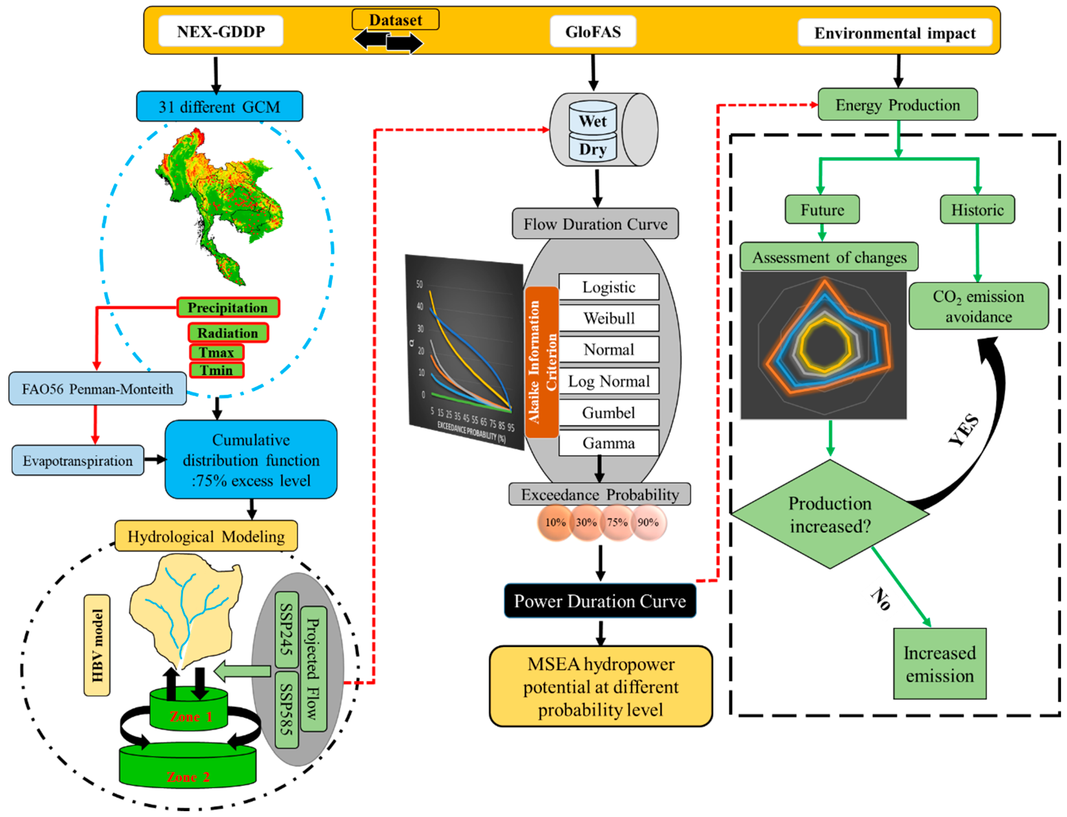
2.1. General Assessment Framework

Figure 1 illustrates the study’s evaluation framework, which consists of a series of steps for analyzing both historical and future periods. For the historical period (H: 1986–2023), the assessment began by dividing the research period into wet and dry phases and deriving Flow Duration Curves (FDC) from available hydrometric stations. Next, RHP production was estimated while considering environmental flow constraints, resulting in the Power Duration Curve (PDC). For future projections, daily data from GCMs are collected to analyze precipitation, solar radiation, and maximum and minimum temperatures for the near future (2024–2061, F₁ period) and the far future (2062–2099, F₂ period). To effectively process these data at each station, the Cumulative Distribution Function (CDF) with a 75% exceedance level is applied to generate a monthly time series for these variables. These are then used as inputs for the HBV (Hydrologiska Byrans Vattenavdelning) hydrological model to predict flow discharge values. Evapotranspiration data required for the HBV model are calculated using the FAO-56 Penman–Monteith equation method [25]. The procedure is repeated for future flow discharge data to compute PDCs for wet and dry periods under the SSP245 and SSP585 scenarios. Finally, the emission rate curves for CO₂ are developed based on PDC results for both historical and future time frames.

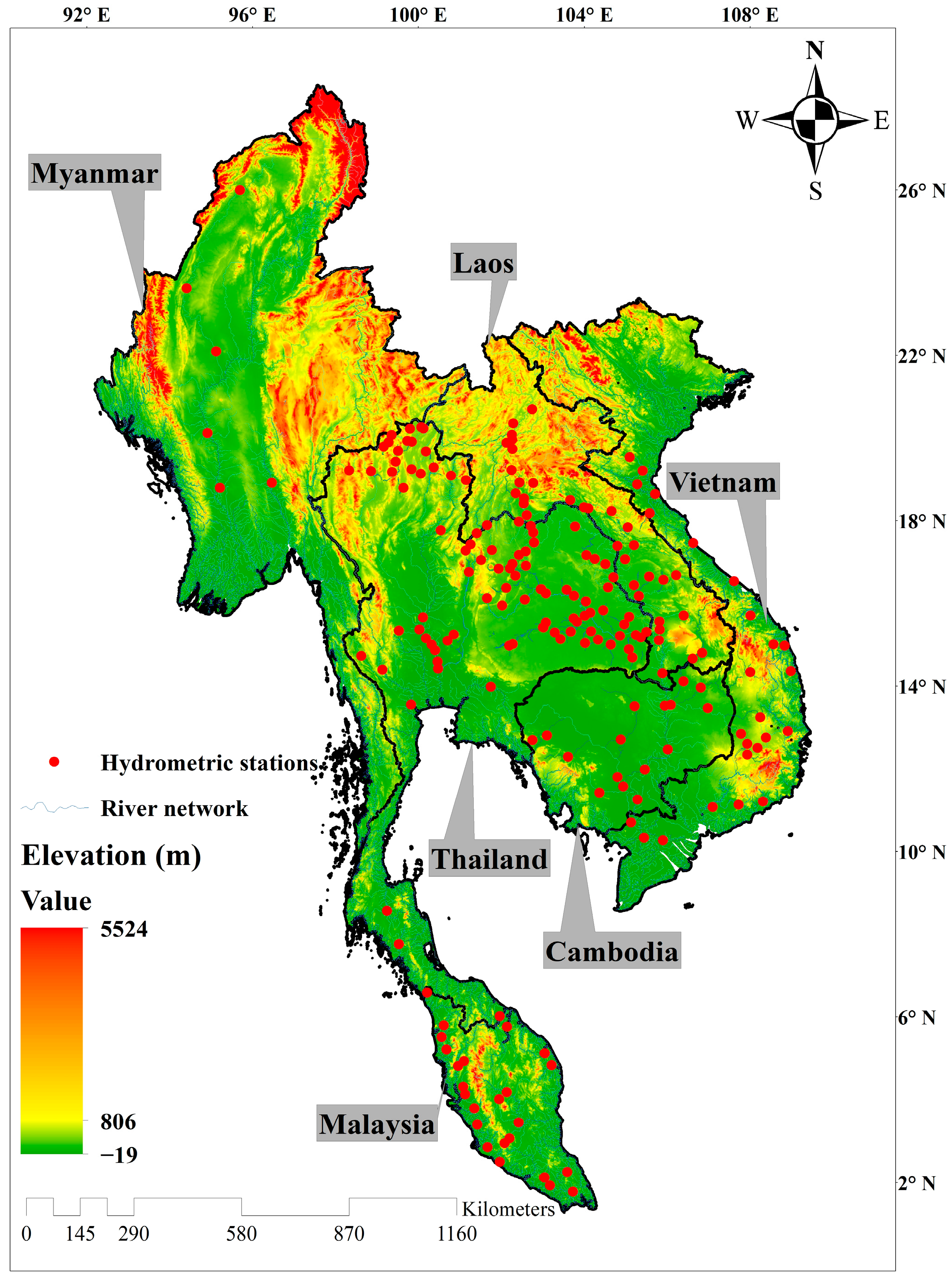
2.2. Study Area and Data

This study focuses on the countries of Mainland Southeast Asia, including Myanmar, Laos, Thailand, Vietnam, Cambodia, and Peninsular Malaysia, as shown in Figure 2. A total of 199 hydrometric stations from the Global Runoff Data Centre [GRDC; https://grdc.bafg.de/ (accessed on 11 November 2024)], an international data centre operating under the auspices of the World Meteorological Organization, have been selected for RHP development. Due to limitations and gaps in the available in situ flow discharge data at these stations, we used the Global Flood Awareness System [GloFAS; http://www.globalfloods.eu/ (accessed on 11 November 2024)] [26] as a benchmark for all stations. In other words, GloFAS data were extracted for each station’s geographical coordinates. The GloFAS is a collaborative initiative under the European Commission’s Copernicus Emergency Management Service (CEMS), integrating a semi-distributed, process-based hydrological tool (LISFLOW) developed by De Roo et al. [27] with the Hydrology Tiled ECMWF Scheme for Surface Exchanges over Land (HTESSEL) [25]. The study analyzed flow discharge data from the GloFAS v4 database, which has a resolution of 0.05° × 0.05° and records dating back to 1979. In this study, GloFAS data were used on a monthly scale, and flow values for each hydrometric station were derived using a correspondence technique known as the point-to-grid method [28].

To predict future flow discharge using the HBV model, data on average temperature, precipitation, and solar radiation are essential. This study utilized a set of 31 GCMs (details provided in Table S1 of the Supplementary Materials) from the NEX-GDDP-CMIP6 database [https://nex-gddp-cmip6.s3.us-west-2.amazonaws.com/index.html (accessed on 11 November 2024)], which has a spatial resolution of 0.25° × 0.25° and a daily temporal resolution [29]. The database provides data for both historical (1950–2014) and future (2015–2100) periods under the SSP245 and SSP585 scenarios. In this study, NEX-GDDP-CMIP6 data were converted to a monthly scale to match the GloFAS time scale and reduce variance. To address scale issues and correct biases, the database employs the Bias Correction and Spatial Disaggregation (BCSD) method, which applies trend-preserving mapping [30,31]. It is important to note that GloFAS flow discharge data were utilized to calculate energy production in the historical period (1986–2023). However, to predict flow discharge in the future period, it was necessary to train and calibrate the HBV model to establish the relationship between flow discharge and climate variables, including precipitation, temperature, and evapotranspiration. In this regard, GloFAS historical flow discharge data, along with climate variables from NEX-GDDP, were instrumental in training and calibrating the HBV model and subsequently predicting future flow discharge for F₁ and F₂ periods.

2.3. Preprocessing and Uncertainty Analysis

Estimating hydropower production from daily and monthly river flow data presents challenges due to uncertainties caused by significant variations [32]. A practical approach to improving accuracy involves utilizing flow discharge patterns in the FDC, which has been shown to reduce hydropower production errors by 30% [32]. The FDC represents the inverse of the cumulative probability distribution of flow discharge, and has been widely applied in RHP production research [33,34,35,36]. A second challenge relates to seasonal variations, which affect both the magnitude and timing of river discharge. To account for this, monthly flow data from GloFAS and the HBV model were categorized into wet and dry periods for each station. In Malaysia, the wet season typically spans from October to March, while the dry season lasts from April to September. In the rest of the area, wet months are generally from May to October, with dry months falling between November and April. The next step involved using FDC to determine the exceedance probability level for each season at all stations. Various probability distributions, including Normal, Log normal, Gumbel, Gamma, Weibull, and Logistic, were examined for developing FDC curves. The best-fitting distribution for each dataset was selected using the Akaike Information Criterion (AIC) [37]. The RHP potential was then evaluated across a full spectrum of flow conditions by using four key exceedance probability levels: 10% (representing the highest potential), 30% (optimal), 75% (balanced), and 90% (base flow). This framework ensures that the assessment reflects the wide range of hydrological conditions experienced in the region, rather than relying on a single average value.

To address uncertainty in GCM climate projections, an ensemble of future climate variables was created. Specifically, the 75th percentile value was chosen from the CDFs of the 31 GCM outputs for each month and required climate variables. This percentile-based approach produced a time series that consistently represents a high-potential climate scenario. By using the 75th percentile, the method intentionally explores a plausible, optimistic future for hydropower generation, based on favorable climate conditions projected by the upper range of GCM models. Finally, the combined monthly time series derived from all 31 GCMs served as input for the HBV model for further analysis and assessment.

2.4. The HBV Hydrological Model

The HBV (Hydrologiska Byrans Vattenavdelning) model was created by the Swedish Meteorological and Hydrological Institute (SMHI) as a conceptual and semi-distributed structure [38,39]. This model was chosen for its capability in modeling discharge flows, which has been widely utilized across 30 countries with varying climates around the globe [40]. The schematic of the HBV model is shown in Figure S1. One of the strengths of the HBV model lies in its simplicity, as it primarily requires precipitation, temperature, and evapotranspiration inputs. This ability has enabled HBV to be utilized in regions with limited data availability. The four main modules of the model structure, which operate in a chain, were the precipitation routine, the soil moisture routine, the base flow routine, and the rapid runoff routine [41]. In this study, 14 HBV parameters (Table S2) were calibrated using the Shuffled Complex Evolution—University of Arizona (SCE-UA) method. The SCE-UA algorithm combines deterministic and probabilistic approaches, and the systematic and competitive evolution of SCE-UA has made it an efficient and powerful algorithm [42]. In this study, the objective function is defined based on the Nash–Sutcliffe Efficiency (NSE), the Kling–Gupta Efficiency (KGE), and the Pearson Correlation Coefficient (PCC), given as follows [43,44,45]:

$$F_{obj}=\mathit{max}\left(\mathrm{N}\mathrm{S}\mathrm{E}·w_1+\mathrm{K}\mathrm{G}\mathrm{E}·w_2+\mathrm{P}\mathrm{C}\mathrm{C}·w_3\right)$$

(1)

$$\begin{array}{ccc}\mathrm{K}\mathrm{G}\mathrm{E}=1-\sqrt{{\left(PCC-1\right)}^2+{\left(B-1\right)}^2+{\left(V-1\right)}^2}& B={\displaystyle \frac{{\mu }_P}{{\mu }_G}}& V={\displaystyle \frac{\raisebox{1ex}{${\delta }_P$}\!\left/ \!\raisebox{-1ex}{${\mu }_P$}\right.}{\raisebox{1ex}{${\delta }_G$}\!\left/ \!\raisebox{-1ex}{${\mu }_G$}\right.}}\end{array}$$

(2)

$$\mathrm{N}\mathrm{S}\mathrm{E}=1-{\displaystyle \frac{{\sum }_{i=1}^n(P_i-G_i{)}^2}{{\sum }_{i=1}^n(G_i-\overline{G}{)}^2}}$$

(3)

$$\mathrm{P}\mathrm{C}\mathrm{C}={\displaystyle \frac{{\sum }_{i=1}^n(G_i-\overline{G})(P_i-\overline{P})}{\sqrt{\left[{\sum }_{i=1}^n(G_i-\overline{G}{)}^2\right]\left[{\sum }_{i=1}^n(P_i-P{)}^2\right]}}}$$

(4)

where G and P represent the GloFAS and predicted flow discharges, respectively, while μ_G and μ_P denote their corresponding mean values. The index weights w are set to 1.0, 0.5, and 0.5 for NSE, KGE, and PCC, respectively. The variable n refers to the number of months. In KGE calculation, the bias (B) and variance (V) components were also calculated, based on the standard deviation (δ) and means of the predicted and GloFAS values.

A combination of historical and projected climate data was used to drive the HBV model. For the calibration (1979–2003) and validation (2004–2014) periods, meteorological inputs and discharge data were sourced from the NEX-GDDP and GloFAS databases. Specifically, precipitation, maximum temperature, minimum temperature, and solar radiation were extracted from the NEX-GDDP. The FAO-56 Penman–Monteith approach was used to calculate evapotranspiration based on solar radiation, and maximum and minimum temperatures [25]. The model was calibrated and validated against flow discharge data from the GloFAS database (Figure S2).

To assess the impacts of climate change, the calibrated HBV model was then forced with meteorological data representing future climate scenarios for the F₁ and F₂ periods. These future inputs, including precipitation, maximum/minimum temperature, and solar radiation, were obtained from the 31 GCMs of the NEX-GDDP dataset. A single time series for each station was generated using the 75th percentile of the GCM output CDFs. After model validation, flow discharge was predicted for all hydrometric stations under the SSP245 and SSP585 scenarios. This approach ensures a direct and consistent connection between the climate change scenarios and the hydrological model inputs. Further details on the HBV modeling process can be found in Hernández et al. [41].

2.5. Potential and Available RHP Production—Environmental Considerations

To estimate RHP production, the methodology first calculates the FDC, followed by the PDC. Several studies have demonstrated the PDC’s ability to distinguish RHP potential [33,46,47]. Subsequently, potential power (PP) production is estimated using Equation (5), which expresses flow discharge based on specific exceedance probability levels. However, instead of directly using PP, available power (AP) production (Equation (6)) is calculated, accounting for environmental flow requirements and the operational constraints of hydropower plants. These two equations are expressed as follows [11]:

$$\mathrm{P}\mathrm{P}=\left[{FD}_P\times g\times Wd\times {\mathsf{\eta }}_T\times {\mathsf{\eta }}_G\times (UH-TH)\right]/{10}^6$$

(5)

$$\mathrm{A}\mathrm{P}=PP\times EFC\times (1-FF)\times (1-MF)$$

(6)

where

• PP: Potential power (MW);
• FD_P: Flow discharge at P exceedance probability level;
• g: Gravity acceleration = 9.8 m·s⁻²;
• Wd: Water density = ~1000 kg·m⁻³;
• η_T: Turbine efficiency = 0.88 [48];
• η_G: Generator efficiency = 0.96 [48];
• UH: Upstream Head (m);
• TH: Turbine Head (m);
• AP: Available power (MW);
• EFC: Environmental Flow Coefficient;
• FF: Forced outage factor;
• MF: Maintenance outage factor.

One of the key variables influencing power calculations of a hydropower plant is the head. As shown in Equation (5), the head is determined as the difference in elevation between the upstream water level and the turbine generator. To obtain this, a Digital Elevation Model (DEM) with a resolution of 0.00836° × 0.00836° was acquired from the NASA/JPL Shuttle Radar Topography Mission (SRTM) dataset [49]. Then, the river network was delineated using HydroRIVERS layers [50], sourced from the HydroSHEDS database (https://www.hydrosheds.org, accessed on 11 November 2024) [51]. Next, flow direction rasters and contour lines were derived from the DEM. A one-kilometer buffer was generated around each hydrometric station, and the hydraulic head at each station was computed as the elevation difference between the station and the highest point within its buffer zone. This study adopted a conservative flow regime, allocating 40% of river discharge to environmental needs [52,53]. To more accurately model turbine performance, operating constraints were incorporated through the forced outage factor (FF) and maintenance factor (MF), set at 0.2917 and 0.12122, respectively [11]. The FF accounted for flow intermittency, while the MF represented downtime due to repairs and maintenance.

2.6. CO₂ Emission Assessment

To assess hydropower’s impact in MSEA, the CO₂ emission reductions (or potential increases) for each RHP were estimated. This study adopts a dual-scenario approach to evaluating CO₂ emissions. The first scenario models the direct effect of replacing fossil fuel-based thermoelectric power plants with hydropower, highlighting potential CO₂ reductions. The second, and likely more significant, scenario considers future conditions under SSP245 and SSP585. In this case, hydropower output may fluctuate due to climate change, requiring thermoelectric plants to compensate for variations in production. As a result, emissions could either increase or decrease. The total hydropower production and CO₂ emission in wet and dry periods can be calculated by the following equations:

$$THP=AP\times ND\times NH$$

(7)

$$DHP={THP}_h-{THP}_f$$

(8)

$$CE=\left\{\begin{array}{l}WEF\times THP, Historical\\ WEF\times DHP, Future\end{array}\right.$$

(9)

where

• THP: Total hydropower production in wet or dry periods (MWh);
• ND: Number of days per period;
• NH: Number of operating hours per day;
• DHP: Declined hydropower production in the future compared to the historical period (MWh);
• CE: CO₂ emissions (tCO₂);
• WEF: Weighted average emissions factor (tCO₂ per MWh).

Equation (7) estimated total hydropower production by incorporating the number of wet and dry days. Turbine operation was assumed to be continuous for 24 h, as any performance reductions due to flow unavailability or maintenance had already been accounted for in the calculations of Equation (6). After determining power production for the historical, F1, and F2 periods, Equation (8) was used to compute the difference in production. The corresponding changes in CO₂ emissions—whether an increase or reduction—were then calculated using Equation (9), with regional emission factors set at 0.7740 (Malaysia), 0.4401 (Thailand), 0.5595 (Laos), 0.94 (Cambodia), 0.72 (Vietnam), and 0.8 (Myanmar) [54,55,56,57,58,59].

3. Results

3.1. Flow/Power Duration Curve in Historical Period

The available flow discharge at 199 hydrometric stations was determined using flow duration curves for exceedance probabilities ranging from 5% to 95% (Figures S3 and S4). The FDCs provided a detailed hydrological fingerprint for each location, with their cumulative distribution functions capturing distinct flow regimes during wet and dry periods. The data indicated that Thailand (94 stations) and Laos (33 stations) exhibited the greatest flow variation during the historical period (1986–2023). To estimate potential power generation, PDCs were derived from the existing FDCs (Figure 3 and Figure 4). Following Punys et al. [32], a 30% exceedance probability was selected as the optimal level for assessing hydropower potential, as it ensured stable flow and reliable energy output for most stations. For some stations, however, this level remained an optimistic target. Additionally, this study evaluated three other exceedance probability levels, including 10%, 75%, and 90%, representing the potential for highest, balanced, and lowest energy production, respectively.

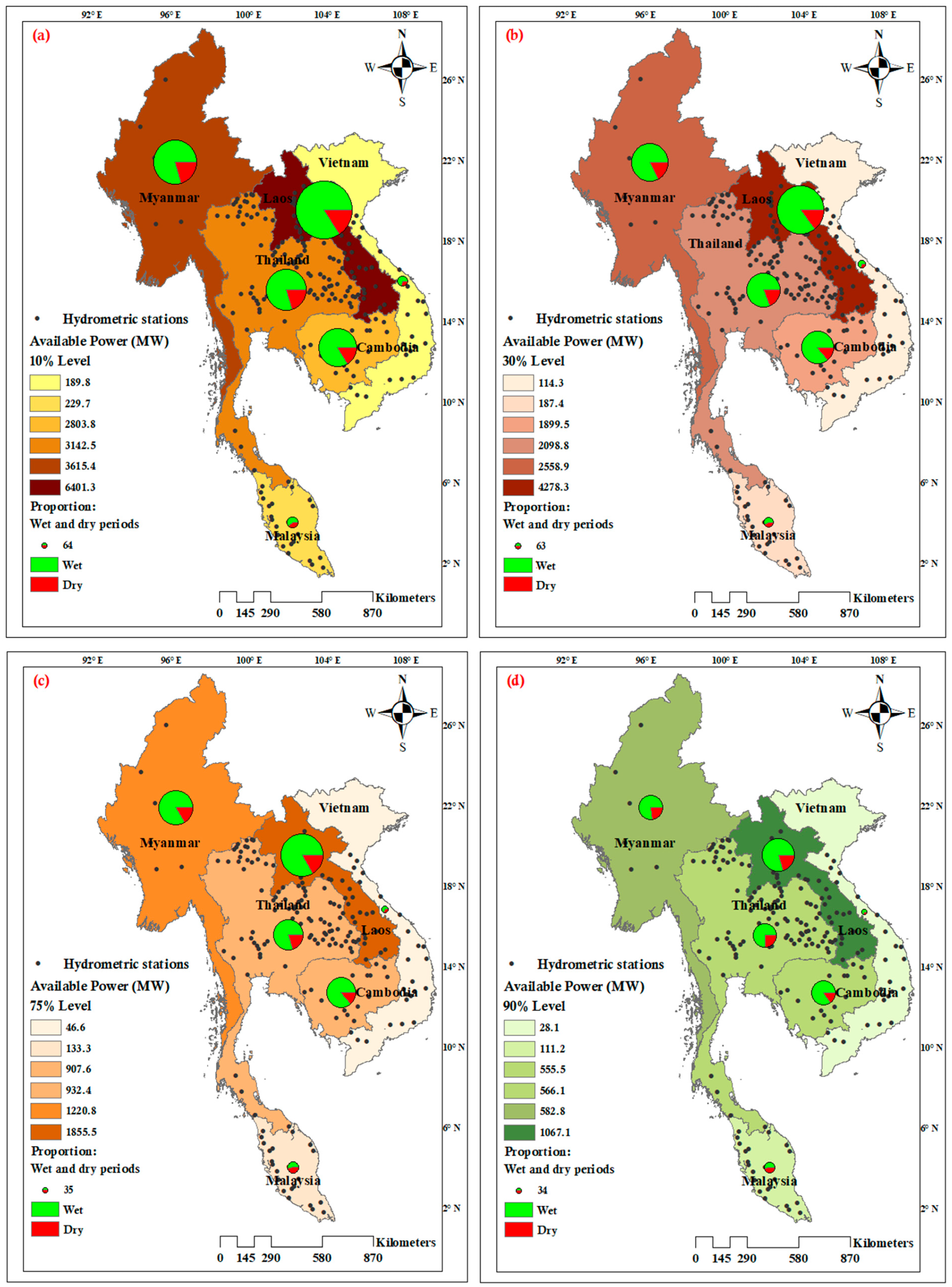
3.2. Current RHP Production

Table 1. Results of RHPs’ production potential at different probability levels of dry period.

	Exceedance Level	Malaysia (MW) 25 *	Myanmar (MW) 6 *	Thailand (MW) 94 *	Laos (MW) 33 *	Vietnam (MW) 25 *	Cambodia (MW) 16 *
Historical (1986–2023)	10%	89.05	736.87	621.53	1016.91	53.34	455.78
	30%	77.00	438.63	389.60	634.17	31.37	269.34
	75%	60.27	196.89	191.62	305.12	13.61	125.25
	90%	53.03	132.28	136.80	211.67	9.13	87.68
SSP245-F1 (2024–2061)	10%	87.80	1034.95	754.45	1487.11	60.69	675.51
	30%	78.20	729.89	495.74	897.41	35.52	484.75
	75%	62.14	340.74	217.49	323.66	13.49	260.43
	90%	52.83	200.85	129.43	167.47	7.44	181.55
SSP245-F2 (2062–2099)	10%	88.44	1228.07	825.92	1609.44	61.32	793.51
	30%	80.00	859.43	542.20	968.84	36.22	567.15
	75%	65.37	393.93	236.78	347.25	14.11	299.46
	90%	56.67	229.12	140.30	179.03	7.95	204.43
SSP585-F1 (2024–2061)	10%	85.52	826.85	562.37	1091.81	42.58	551.51
	30%	76.00	579.11	376.00	669.88	25.13	388.68
	75%	59.55	266.78	171.26	250.97	10.44	212.30
	90%	49.78	155.82	104.17	134.19	6.36	151.10
SSP585-F2 (2062–2099)	10%	83.09	1210.45	618.41	1165.53	45.31	750.82
	30%	74.37	851.29	419.09	723.13	26.83	553.25
	75%	59.57	394.98	197.74	278.77	11.12	313.75
	90%	50.87	231.83	124.31	152.81	6.81	226.32

Note: * Number of hydrometric stations.

and

Table 2. Results of RHPs’ production potential at different probability levels of wet period.

	Exceedance Level	Malaysia (MW) 25 *	Myanmar (MW) 6 *	Thailand (MW) 94 *	Laos (MW) 33 *	Vietnam (MW) 25 *	Cambodia (MW) 16 *
Historical (1986–2023)	10%	140.57	2878.49	2520.92	5384.35	136.43	2347.97
	30%	110.43	2120.36	1709.21	3644.17	82.94	1630.15
	75%	73.02	1023.93	740.74	1550.41	33.00	782.38
	90%	58.12	450.50	418.67	855.38	18.94	478.45
SSP245-F1 (2024–2061)	10%	138.00	3130.58	2448.04	5297.85	126.49	2763.26
	30%	112.87	2072.41	1660.94	3533.31	78.95	1746.48
	75%	73.44	835.50	731.84	1464.52	31.28	659.16
	90%	54.06	441.52	419.32	798.33	17.21	340.50
SSP245-F2 (2062–2099)	10%	148.30	3617.01	2738.04	5816.67	131.56	3327.56
	30%	121.23	2595.94	1846.42	3899.66	84.10	2065.87
	75%	78.68	1176.10	806.26	1640.21	34.86	742.65
	90%	57.74	554.74	459.64	905.24	18.40	368.74
SSP585-F1 (2024–2061)	10%	126.46	2513.16	1971.70	4194.95	105.88	2508.74
	30%	107.06	1860.25	1403.78	2956.09	69.90	1497.81
	75%	73.95	924.10	680.82	1381.75	31.24	579.44
	90%	55.64	503.64	415.06	818.35	18.58	325.42
SSP585-F2 (2062–2099)	10%	131.99	3960.81	2299.68	4732.77	114.96	3623.80
	30%	108.16	2986.24	1690.12	3456.59	81.82	2313.31
	75%	71.26	1582.23	872.72	1744.81	39.25	909.61
	90%	53.41	954.08	555.02	1088.78	20.61	488.98

Note: * Number of hydrometric stations.

summarize the potential for RHP production across different probability levels and during dry and wet periods, presenting the aggregate potential of all stations within each country. Despite having only 33 stations, Laos consistently yielded the highest total energy production across all probability levels, outperforming Thailand, which has a much larger network of 94 stations. This strong performance in Laos is attributed to its high flow discharge rate (Figures S3 and S4), a capacity also highlighted in previous research [60]. Similarly, Myanmar, with just six stations, demonstrated substantial hydropower potential. At the optimal level (30% probability), total MSEA production during the wet and dry seasons reached 9297.26 (MW) and 1840.10 (MW), respectively. A shift to the balanced level (75% probability) resulted in a substantial decline, with wet and dry season outputs dropping by 54.8% and 51.5%, respectively. Figure 5 illustrates the spatial variation in aggregate wet and dry season power production. The most pronounced seasonal imbalance was observed in Laos and Cambodia, where 84% of their maximum total production occurred during the wet season (Figure 5a). In contrast, Malaysia exhibited the most balanced seasonal distribution, with the wet season contributing 61% and the dry season 39%. Notably, across all assessed probability levels, Malaysia experienced the least seasonal variation, with only a 4% difference at the 90% level. At the balanced level, MSEA’s total production capacity was 5096.21 MW (Figure 5c), with Laos contributing the largest share (36.4%) and Vietnam the smallest (0.91%). These findings highlight Laos’ role as a major hydropower producer in the region, supplying a portion of the electricity consumed annually by Thailand, Vietnam, and Cambodia [61].

3.3. Projected Change in Flow Discharge

Flow discharge during the F₁ and F₂ timeframes was simulated using the HBV hydrological model. The model’s performance was evaluated using PCC and KGE. The model was initially calibrated using data from 1979 to 2003, followed by a validation phase using data from 2004 to 2014. The validation results, presented in Table S3, indicate a range in PCC from 0.745 to 0.994 and in KGE from 0.701 to 0.986. These values are generally interpreted as being within satisfactory limits for accurately estimating flow discharge [9,62].

Figure 6 illustrates the average percentage changes in wet and dry season discharge compared to historical conditions. The projected effects of climate change on flow discharge reveal a complex pattern, with substantial variation across countries and probability levels. Malaysia showed the least influence of climate change, whereas Myanmar and Cambodia experienced the greatest variation. In Malaysia, the wet season response was mixed (Figure 6a). Under the SSP245-F₁ scenario, extreme and base flows (10% and 90%) decreased, while optimal and balanced levels (30% and 75%) increased. Under SSP245-F₂, wet season discharge increased across all assessed levels, ranging from 2% to 10%. However, in the far future, under the most severe scenario (SSP585), Malaysia’s flow discharge declined during both wet and dry seasons. Notably, under SSP585-F₁, reductions were observed at all levels except the balanced level.

In Myanmar, only the most severe scenario, SSP585-F₁, led to reduced flows in both the wet season (at the 10% and 30% levels) and the dry season (at the 10% and 90% levels). However, under all other scenarios, a significant increase in flow was observed compared to historical data (Figure 6b). The largest percentage increase occurred at the base flow level (90%), rising by 52%, followed by a 40% increase in the optimal and balanced flow rate. In Thailand, the wet season showed an overall average reduction of 3.4% and 14.7% under the SSP245-F₁ and SSP585-F₁ scenarios, respectively (Figure 6c). Meanwhile, under SSP245, the dry season experienced an overall average increase of 17.8% and 28.6% in the F₁ and F₂ periods, respectively. Across Laos and Vietnam, base flow generally declined in most scenarios, except for the wet season under SSP585-F₂, with average declines of 13% in Laos and 16.6% in Vietnam. In Cambodia, increases were observed across most probability levels (Figure 6d), with the dry season showing the most pronounced change, rising by 96.8% and 112.6% under the SSP245-F₂ and SSP585-F₂ scenarios, respectively.

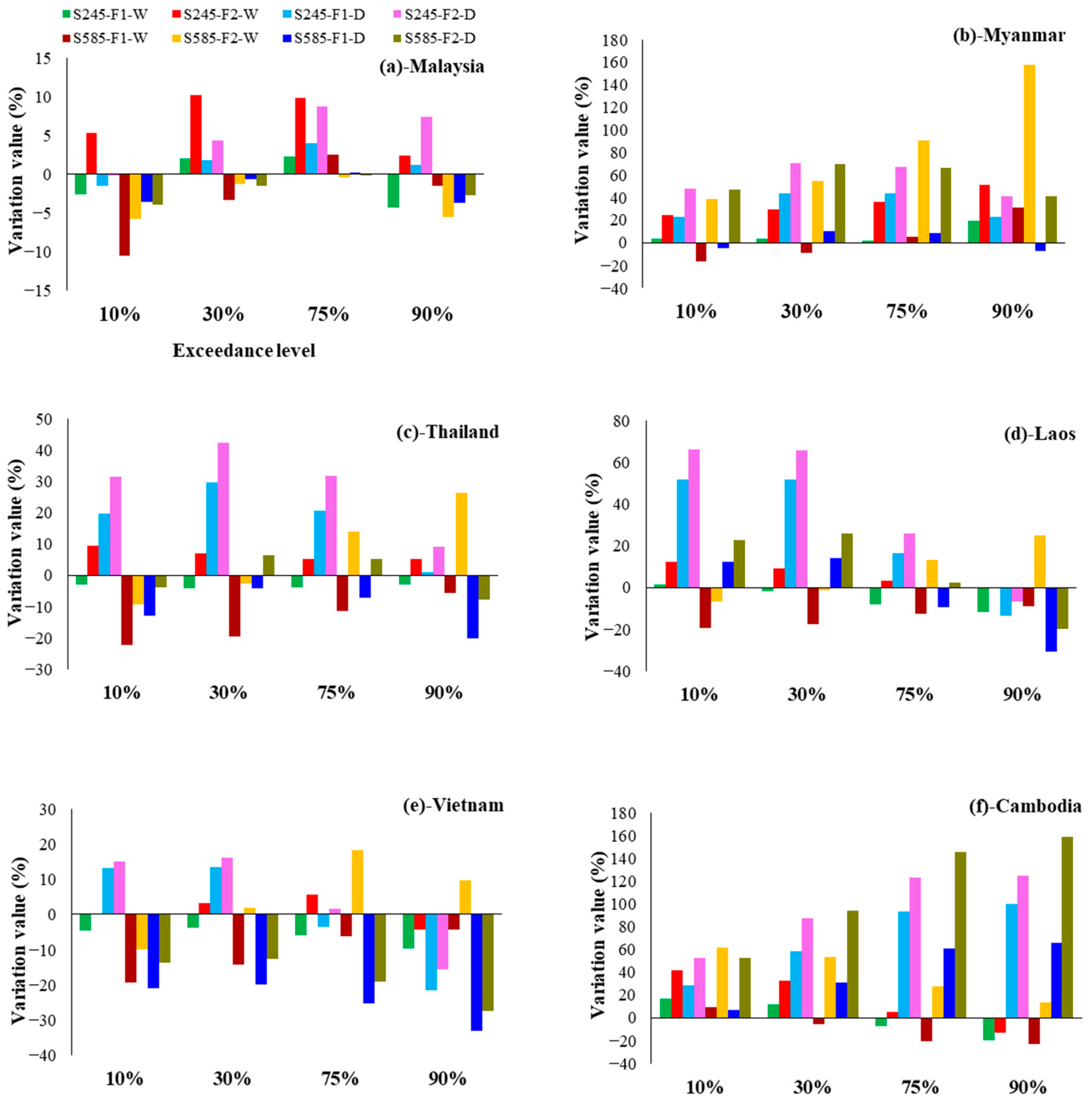
3.4. Climate Change Impact on RHP Production

Table 1 and Table 2 present the projected impacts of climate change on RHP potential across various scenarios and flow probability levels. In Malaysia, only minimal decreases in energy output were observed at the 10% flow level for both wet and dry seasons under SSP245 and SSP585, with the exception of a wet season increase in SSP245-F₂. For optimal production (30% level), SSP245 generally led to increases, whereas SSP585 resulted in declines. Figure 7 provides a visual comparison of future and historical hydropower potential by country. While Malaysia showed no increase at the 10% level, Myanmar exhibited a general upward trend in both wet and dry seasons at this level, except for the wet season under SSP585-F₁. Moreover, the potential to achieve optimal energy output in the wet season declined during F₁ but recovered in F₂ under both scenarios. In contrast, optimal dry season production increased significantly, with average gains of 49% in the near future and 95% in the far future (Figure 7b).

In Thailand, during the initial projection period (F₁), wet season energy output declined across all three flow levels (10%, 30% and 75%) under both climate change scenarios (Figure 7c). A similar trend was observed in Laos, where wet season production decreased at all probability levels in the F₁ period, with modest reductions under SSP245 and more substantial declines under SSP585. In contrast, dry season production in Laos showed mixed results: increases were observed at the 10%, 30%, and 75% levels under SSP245, and at the 10% and 30% levels under SSP585, while other levels and periods showed declines (Figure 7d). In Vietnam, optimal dry season energy production increased by 13–15% under SSP245 but declined by 14–19.8% under SSP585. For the wet season, production at the balanced level slightly decreased in F₁, followed by a modest recovery in F₂ under both climate scenarios. Cambodia followed a pattern similar to its earlier flow discharge trends (Figure 7f), with a notable increase in energy production across all probability levels during the dry season.

3.5. Spatial Analysis of Optimal Energy Production Potential

To further assess MSEA energy production under climate change scenarios, this section examines the spatial distribution of projected changes in optimal hydropower production. Figure 8 presents future energy production changes at the 30% probability level for 199 hydrometric stations. As shown in Figure 8a, under the SSP245 scenario for the near future, neither Cambodia nor Myanmar experienced a decline in energy production. Instead, both countries showed overall increases, with Cambodia’s 16 stations adding 331.75 MW and Myanmar’s six stations contributing 243.31 MW. In contrast, the most noticeable decreases were observed in central regions, including parts of Laos and Thailand, as well as southern Malaysia. Although specific stations in Laos and Thailand recorded reductions of 25.82 MW and 12.6 MW, respectively, aggregate production from other stations increased by 178.19 MW in Laos and 70.47 MW in Thailand.

By the second half of the century, under the SSP245 scenario (Figure 8b), this trend reversed, with most stations showing an increase of at least 25 MW. In contrast, the F₁ period under the SSP585 scenario presented a markedly different outcome. At 153 stations, optimal energy production declined by a total of 1133.18 (MW) (Figure 8c). Under this high-emission scenario, only a few localized areas, such as western Malaysia and southern Cambodia, experienced increases in production. During the F₂ period of the SSP585 scenario (Figure 8d), the spatial pattern resembled that of the F₁ period under SSP245. In this phase, stations in central Laos and Thailand, as well as southern Malaysia, showed reductions in energy production. The most notable increases in energy production reached up to 15 MW, with the highest gains observed in Myanmar.

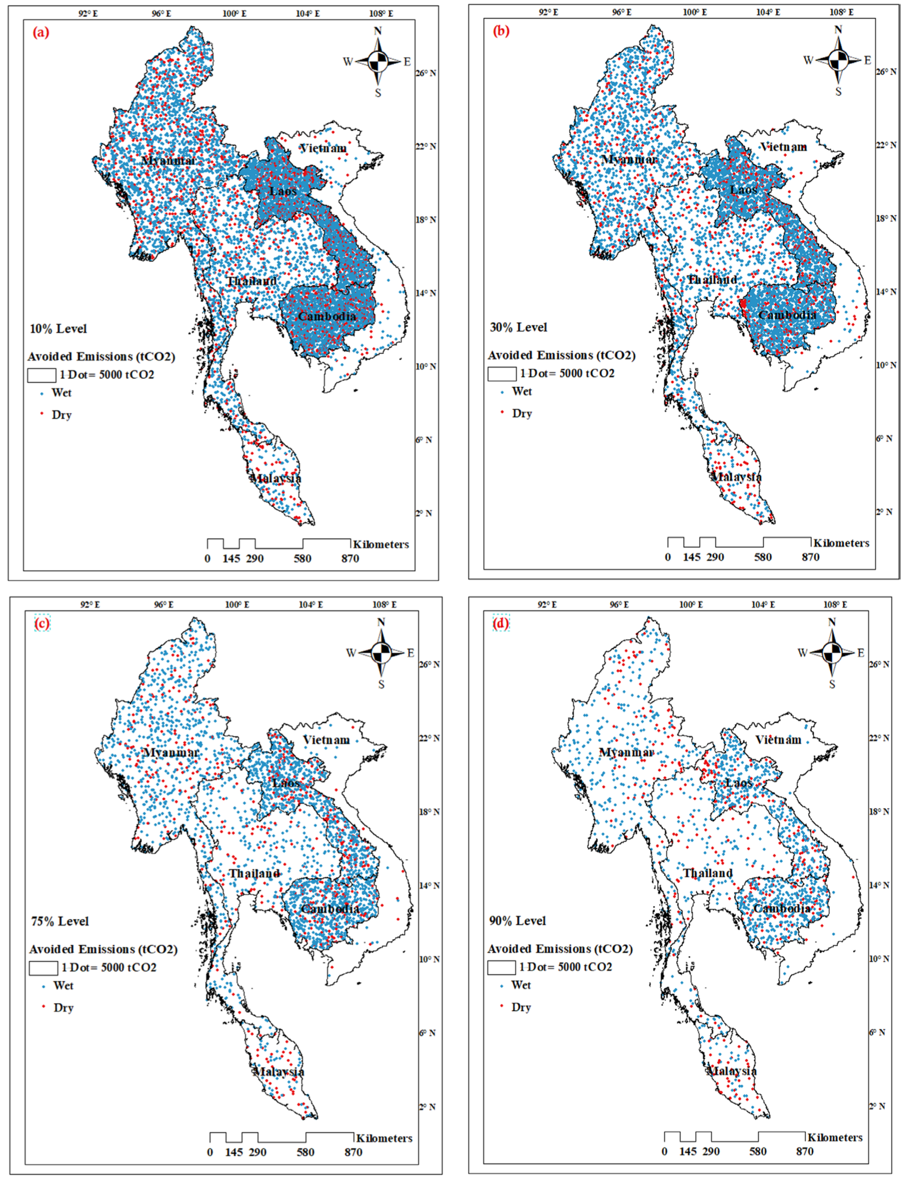
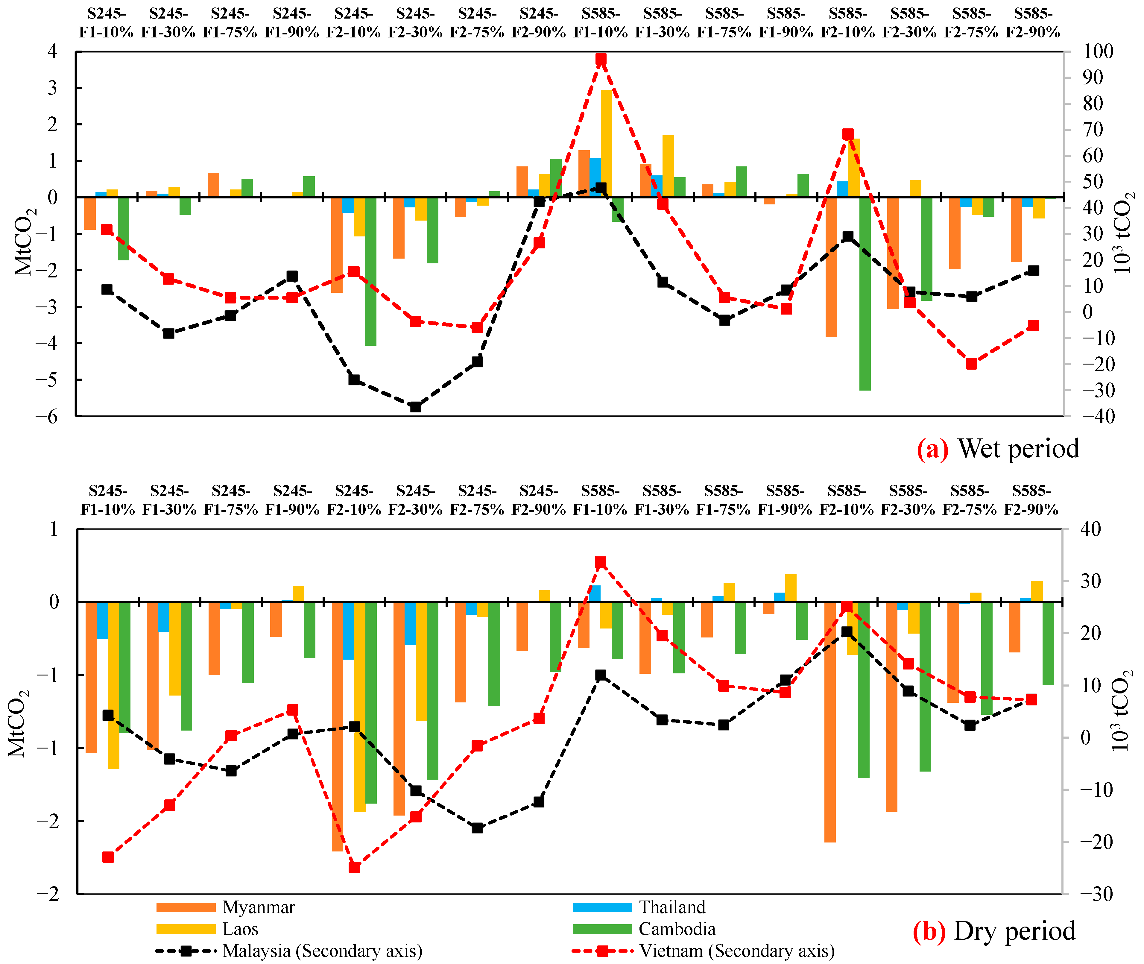
3.6. Potential Changes in CO₂ Emissions

All MSEA countries are committed to reducing emissions under the guidelines of the Paris Agreement and, therefore, urgently need to lower CO₂ emissions. Specific 2030 CO₂ emission reduction commitments include: Malaysia (45%), Thailand (20%), Laos (60%), Vietnam (8%), Myanmar (50%), and Cambodia (42%) [63]. Yet, in 2022, fossil-based power plants remained a significant energy source, contributing considerable emissions across MSEA (Table S4) [64]. In this section, the emission reduction potential from RHPs is analyzed. Figure 9 shows the annual CO₂ emission avoidance achieved through hydropower operation at various exceedance probability levels, relative to historical data. At the highest level of energy production (10% level), CO₂ avoidance ranged from 0.6 to 15.8 Mt, with the highest reductions in Laos (15.8 Mt), followed by Cambodia (11.6 Mt). Vietnam and Malaysia recorded the lowest rates, at 0.6 Mt and 0.78 Mt, respectively.

At the optimal production level, the total CO₂ emission reduction was 32.5 Mt, 15.1 Mt lower than at the 10% level. According to Figure 9b, Malaysia demonstrated the highest contribution from the dry season to the overall emission reduction (41.2%). As the exceedance probability increased to 75% and 90%, the total emission reductions declined, while the dry season’s share in most regions increased. Since Cambodia and Laos had the highest energy production, they also recorded the highest emission reduction rates, as shown in Figure 9. Despite having only six hydrometric stations, Myanmar showed an emission reduction range of 2.05 to 12.73 Mt, with the wet season accounting for an average of 81.2% of the total.

Figure 10 illustrates the changes in CO₂ emissions under different climate scenarios. Negative values represent avoided emissions (relative to historical baselines), whereas positive values indicate increased emissions due to energy shortfalls. It is assumed that reduced hydropower generation caused by climate change would be offset by fossil-based power plants, leading to higher CO₂ emissions. Among MSEA countries, Malaysia and Vietnam recorded the lowest levels of emission avoidance in both the wet and dry seasons. For Malaysia, CO₂ avoidance was observed across all probability levels and periods under SSP245, except during F₁ at the 10% and 90% levels, and F₂ at the 90% level. Vietnam faced particularly critical conditions during the wet season, with aggregate emission avoidance of only 0.01 Mt under SSP245-F₂ (30% and 75% levels) and 0.025 Mt under SSP585-F₂ (75% and 90% levels). In all other wet season scenarios, Vietnam experienced net CO₂ emissions due to reduced hydropower production.

For the wet season at the optimal level in SSP245-F₁, only Malaysia and Cambodia achieved emission avoidance, totaling 0.491 Mt. However, in the second half of the century under SSP245, all countries recorded positive avoidance, amounting to 4.4 Mt across MSEA. Under SSP585, 3.82 Mt of CO₂ emissions were required to compensate for the reduction in optimal energy production in MSEA. Additionally, under SSP245 at the balanced level during F₁, all MSEA countries, except Malaysia, produced 1.41 Mt of CO₂ emissions. During the dry season, optimal production under the SSP245 improved emission avoidance by 2.75 Mt and in F₁ and 3.8 Mt in F₂. At the balanced level, SSP245 led to an emission avoidance increase of 1.15 Mt and 1.6 Mt in F₁ and F₂, respectively.

4. Discussion

This study assessed the potential of RHPs in MSEA. Energy supply in the region currently relies heavily on large dams and reservoirs, which are associated with environmental and ecological concerns [23]. RHPs have been proposed as a potential regional solution to reduce reliance on large-scale reservoir development. Although limited in scale and unable to fully replace energy generation from conventional reservoir plants, RHPs offer notable advantages, including lower construction costs and reduced labor requirements. Thus, their deployment has been found feasible in MSEA, a region characterized by a dense network of main and tributary rivers. Moreover, the construction of RHPs has been shown to promote local development, contributing to economic and social growth even in resource-scarce areas [53,65,66]. However, careful planning and deployment are essential, as the success of these small-scale projects depends on factors such as social acceptance, legal and geopolitical contexts, competing water use priorities, and the protection of local ecosystems [53].

The comparison of this study’s results with previous research was limited by a scarcity of studies on RHPs in MSEA. Nevertheless, commonalities with previous work were highlighted. The results of river flow changes under the two scenarios, SSP245 and SSP585, showed different ranges due to the assessment of four discharge levels: minimum, optimal, balanced, and maximum. Other studies also reported similarly wide ranges in Malaysia [67,68], Cambodia [69], Laos [70], and Myanmar [71]. An increase in flow discharge in Vietnam was reported by Khoi et al. [72], ranging from 1.8 to 13% under SSP245 and from 0.1 to 19.6% under SSP585. This increase observed in the present study was also within a similar range, namely 0.2 to 16.2% (SSP245) and 1.9 to 18.2% (SSP585).

In terms of the energy production potential in MSEA, Thailand was a key focus, with RHPs assessed at 94 hydrometric stations. A potential of 2098.81 MW at historical and optimal levels was identified, exceeding the targets outlined in Thailand’s hydropower development plan. The Thai government previously planned to exploit hydropower in three phases: 2008–2011 (165 MW), 2012–2016 (281 MW), and 2017–2022 (324 MW) [73]. The government also intends to promote small-scale RHPs for irrigation purposes [74,75]. Myanmar was likewise found to have significant production potential across six stations, consistent with the findings of Tang et al. [6]. A primary component of Myanmar’s energy strategy has been to attract foreign investment to rapidly expand its hydropower sector [76]. A major challenge, also noted in this study and previous work [74], is the seasonal variation in power production; during the dry season, energy output at optimal production levels dropped to about one-fifth of that in the wet season. The production potential was also evaluated at 25 stations in Malaysia, as an alternative to fossil power plants and diesel generators. Given the popularity and reliability of RHPs in Malaysia, they are particularly suitable for most areas, especially remote areas [77,78,79]. This study focuses only on Peninsular Malaysia, whereas East Malaysia is estimated to have four times greater hydropower potential [6].

5. Research Limitations

The limitations of this research can be categorized into several aspects, each affecting specific components of the study. Firstly, the unavailability of observed flow discharge data from gauging stations posed a major challenge. As a result, the use of reanalyzed datasets such as GloFAS may have introduced errors and uncertainties. Secondly, the method used to determine hydraulic head, based on elevation data and river network analysis, differs from direct in situ measurements, introducing another layer of uncertainty. Finally, the application of the HBV model for discharge estimation also introduced potential limitations, as previous studies have shown that the HBV model has reduced accuracy in capturing hydrological characteristics in basins affected by human activities [80].

6. Conclusions and Future Directions

This study explored the application of 199 RHPs across MSEA. The primary focus was to evaluate their power production under four operational levels, including minimum, optimal, balanced, and maximum, for both the current climate and two future climate scenarios (SSP245 and SSP585). To support sustainable development and ensure a holistic assessment, environmental flow constraints and CO₂ emission impacts were also considered. The aggregate power production potential under current conditions varied significantly by country, with production ranges of 111.15–229.62 MW (Malaysia), 582.78-3615.36 MW (Myanmar), 555.47–3142.46 MW (Thailand), 1067.05–6401.25 MW (Laos), 28.07–189.77 MW (Vietnam), and 566.13–2803.75 MW (Cambodia). The projected impacts of climate change on power production were found to be highly variable, depending on both the scenario and country. Under SSP245, production at the optimal level showed an average increase of 5.9% in the near future and 19% in the far future. Conversely, under SSP585, production declined by 9.2% in the near term but increased by 15.3% in the longer term. In terms of emissions, RHP development in MSEA contributed to the avoidance of 32.5 Mt of CO₂ emissions at the optimal operational level. Emission avoidance increased by 8.3% and 25.3% under SSP245 (F₁ and F₂, respectively) compared to the historical period. Under SSP585, avoidance decreased by 8.6% in the near term (F₁) but was comparable to SSP245 in the far future (F₂).

Building on these findings, future research should aim to refine the projections and translate them into actionable energy strategies. To address climate-related uncertainties, more advanced hydrological models, coupled with improved datasets, could yield more reliable power generation estimates [81]. Beyond assessing technical potential, it is also crucial to evaluate the economic viability of these projects by considering factors such as power purchase agreements, grid infrastructure, and tax regimes. Such economic analysis would support the use of multi-objective optimization to better balance energy production goals with financial constraints. Lastly, to create a truly comprehensive energy plan for the region, these RHP assessments should be integrated with evaluations of other renewable energy sources, thereby supporting the creation of a resilient and diversified energy portfolio for MSEA.

References

1. Paris 2024. Available online: https://www.iea.org/reports/co2-emissions-in-2023 (accessed on 11 November 2024).
2. UNCC: United Nations Climate Change Annual Report 2020. 2021. Available online: https://unfccc.int/sites/default/files/resource/UNFCCC_Annual_Report_2020.pdf (accessed on 11 November 2024).
3. Zhang, C.; Chen, S.; Qiao, H.; Dong, L.; Huang, Z.; Ou, C. Small hydropower sustainability evaluation for the countries along the Belt and Road. Environ. Dev. 2020, 34, 100528. [Google Scholar] [CrossRef]
4. Grodzicki, T.; Jankiewicz, M. The impact of renewable energy and urbanization on CO2 emissions in Europe–Spatio-temporal approach. Environ. Dev. 2022, 44, 100755. [Google Scholar] [CrossRef]
5. Jakimavičius, D.; Adžgauskas, G.; Šarauskienė, D.; Kriaučiūnienė, J. Climate change impact on hydropower resources in gauged and ungauged Lithuanian river catchments. Water 2020, 12, 3265. [Google Scholar] [CrossRef]
6. Tang, S.; Chen, J.; Sun, P.; Li, Y.; Yu, P.; Chen, E. Current and future hydropower development in Southeast Asia countries (Malaysia, Indonesia, Thailand and Myanmar). Energy Policy 2019, 129, 239–249. [Google Scholar] [CrossRef]
7. Lau, H.C.; Zhang, K.; Bokka, H.K.; Ramakrishna, S. A review of the status of fossil and renewable energies in Southeast Asia and its implications on the decarbonization of ASEAN. Energies 2022, 15, 2152. [Google Scholar] [CrossRef]
8. Sakti, A.D.; Rohayani, P.; Izzah, N.A.; Toya, N.A.; Hadi, P.O.; Octavianti, T.; Harjupa, W.; Caraka, R.E.; Kim, Y.; Avtar, R.; et al. Spatial integration framework of solar, wind, and hydropower energy potential in Southeast Asia. Sci. Rep. 2023, 13, 340. [Google Scholar] [CrossRef] [PubMed]
9. Mosier, T.M.; Sharp, K.V.; Hill, D.F. The Hydropower Potential Assessment Tool (HPAT): Evaluation of run-of-river resource potential for any global land area and application to Falls Creek, Oregon, USA. Renew. Energy 2016, 97, 492–503. [Google Scholar] [CrossRef]
10. Balat, H. A renewable perspective for sustainable energy development in Turkey: The case of small hydropower plants. Renew. Sustain. Energy Rev. 2007, 11, 2152–2165. [Google Scholar] [CrossRef]
11. Michels-Brito, A.; Rodriguez, D.A.; Junior, W.L.C.; de Souza Vianna, J.N. The climate change potential effects on the run-of-river plant and the environmental and economic dimensions of sustainability. Renew. Sustain. Energy Rev. 2021, 147, 111238. [Google Scholar] [CrossRef]
12. Arias, M.E.; Farinosi, F.; Lee, E.; Livino, A.; Briscoe, J.; Moorcroft, P.R. Impacts of climate change and deforestation on hydropower planning in the Brazilian Amazon. Nat. Sustain. 2020, 3, 430–436. [Google Scholar] [CrossRef]
13. Tobias, W.; Manfred, S.; Klaus, J.; Massimiliano, Z.; Bettina, S. The future of Alpine Run-of-River hydropower production: Climate change, environmental flow requirements, and technical production potential. Sci. Total Environ. 2023, 890, 163934. [Google Scholar] [CrossRef]
14. Mohsin, M.; Orynbassarov, D.; Anser, M.K.; Oskenbayev, Y. Does hydropower energy help to reduce CO2 emissions in European Union countries? evidence from quantile estimation. Environ. Dev. 2023, 45, 100794. [Google Scholar] [CrossRef]
15. Destek, M.A.; Aslan, A. Disaggregated renewable energy consumption and environmental pollution nexus in G-7 countries. Renew. Energy 2020, 151, 1298–1306. [Google Scholar] [CrossRef]
16. Almeida, R.M.; Fleischmann, A.S.; Brêda, J.P.; Cardoso, D.S.; Angarita, H.; Collischonn, W.; Forsberg, B.; García-Villacorta, R.; Hamilton, S.K.; Hannam, P.M.; et al. Climate change may impair electricity generation and economic viability of future Amazon hydropower. Glob. Environ. Change 2021, 71, 102383. [Google Scholar] [CrossRef]
17. Qin, P.; Xu, H.; Liu, M.; Du, L.; Xiao, C.; Liu, L.; Tarroja, B. Climate change impacts on Three Gorges Reservoir impoundment and hydropower generation. J. Hydrol. 2020, 580, 123922. [Google Scholar] [CrossRef]
18. Arias, M.E.; Cochrane, T.A.; Kummu, M.; Lauri, H.; Holtgrieve, G.W.; Koponen, J.; Piman, T. Impacts of hydropower and climate change on drivers of ecological productivity of Southeast Asia’s most important wetland. Ecol. Model. 2014, 272, 252–263. [Google Scholar] [CrossRef]
19. Aroonrat, K.; Wongwises, S. Current status and potential of hydro energy in Thailand: A review. Renew. Sustain. Energy Rev. 2015, 46, 70–78. [Google Scholar] [CrossRef]
20. Purwanto, W.W.; Afifah, N. Assessing the impact of techno socioeconomic factors on sustainability indicators of microhydro power projects in Indonesia: A comparative study. Renew. Energy 2016, 93, 312–322. [Google Scholar] [CrossRef]
21. Yah, N.F.; Oumer, A.N.; Idris, M.S. Small scale hydro-power as a source of renewable energy in Malaysia: A review. Renewable and Sustainable Energy Rev. 2017, 72, 228–239. [Google Scholar] [CrossRef]
22. Siala, K.; Chowdhury, A.K.; Dang, T.D.; Galelli, S. Solar energy and regional coordination as a feasible alternative to large hydropower in Southeast Asia. Nat. Commun. 2021, 12, 4159. [Google Scholar] [CrossRef]
23. MRC. Mekong River Commission for Sustainable Development (MRC)-Hydropower. 2020. Available online: https://www.mrcmekong.org (accessed on 5 December 2024).
24. Thui, P.C. Cambodia Halts Mainstream Mekong River Dam Plans for 10 Years, Official Says. 2020. Available online: https://www.reuters.com/article/us-mekong-river-cambodia/cambodia-halts-mainstream-mekong-river-dam-plans-for-10-years-official-says-idUSKBN215187/ (accessed on 5 December 2024).
25. Allen, R.G.; Pereira, L.S.; Raes, D.; Smith, M. FAO Irrigation and Drainage Paper No. 56; Food and Agriculture Organization of the United Nations: Rome, Italy, 1998; Volume 56, p. e156. [Google Scholar]
26. Grimaldi, S.; Salamon, P.; Disperati, J.; Zsoter, E.; Russo, C.; Ramos, A.; Carton De Wiart, C.; Barnard, C.; Hansford, E.; Gomes, G.; et al. River Discharge and Related Historical Data from the Global Flood Awareness System, v4.0; European Commission, Joint Research Centre (JRC) Climate Copernicus EU/CDSAPP: Brussels, Belgium, 2022. [Google Scholar]
27. De Roo, A.; Wesseling, C.; Van Deursen, W. Physically based river basin modelling within a GIS: The LISFLOOD model. Hydrol. Process. 2000, 14, 1981–1992. [Google Scholar] [CrossRef]
28. Lei, H.; Zhao, H.; Ao, T. Ground validation and error decomposition for six state-of-the-art satellite precipitation products over mainland China. Atmos. Res. 2022, 269, 106017. [Google Scholar] [CrossRef]
29. Thrasher, B.; Wang, W.; Michaelis, A.; Melton, F.; Lee, T.; Nemani, R. NASA global daily downscaled projections, CMIP6. Sci. Data 2022, 9, 262. [Google Scholar] [CrossRef] [PubMed]
30. Wood, A.W.; Leung, L.R.; Sridhar, V.; Lettenmaier, D. Hydrologic implications of dynamical and statistical approaches to downscaling climate model outputs. Clim. Change 2004, 62, 189–216. [Google Scholar] [CrossRef]
31. Thrasher, B.; Maurer, E.P.; McKellar, C.; Duffy, P.B. Bias correcting climate model simulated daily temperature extremes with quantile mapping. Hydrol. Earth Syst. Sci. 2012, 16, 3309–3314. [Google Scholar] [CrossRef]
32. Punys, P.; Kvaraciejus, A.; Dumbrauskas, A.; Šilinis, L.; Popa, B. An assessment of micro-hydropower potential at historic watermill, weir, and non-powered dam sites in selected EU countries. Renew. Energy 2019, 133, 1108–1123. [Google Scholar] [CrossRef]
33. Vogel, R.M.; Fennessey, N.M. Flow duration curves II: A review of applications in water resources planning 1. JAWRA J. Am. Water Resour. Assoc. 1995, 31, 1029–1039. [Google Scholar] [CrossRef]
34. Hänggi, P.; Weingartner, R. Variations in discharge volumes for hydropower generation in Switzerland. Water Resour. Manag. 2012, 26, 1231–1252. [Google Scholar] [CrossRef]
35. Wagner, T.; Themeßl, M.; Schüppel, A.; Gobiet, A.; Stigler, H.; Birk, S. Impacts of climate change on stream flow and hydro power generation in the Alpine region. Environ. Earth Sci. 2017, 76, 1–22. [Google Scholar] [CrossRef]
36. Kuriqi, A.; Pinheiro, A.N.; Sordo-Ward, A.; Garrote, L. Flow regime aspects in determining environmental flows and maximising energy production at run-of-river hydropower plants. Appl. Energy 2019, 256, 113980. [Google Scholar] [CrossRef]
37. Akaike, H. Information theory and an extension of the maximum likelihood principle. In Selected Papers of Hirotugu Akaike; Springer: New York, NY, USA, 1998; pp. 199–213. [Google Scholar]
38. Bergström, S. The HBV Model–Its Structure and Applications; SMHI: Norrköping, Sweden, 1992. [Google Scholar]
39. Bergström, S. Development and Application of a Conceptual Runoff Model for Scandinavian Catchments; SMHI: Norrköping, Sweden, 1976. [Google Scholar]
40. Lindström, G.; Johansson, B.; Persson, M.; Gardelin, M.; Bergström, S. Development and test of the distributed HBV-96 hydrological model. J. Hydrol. 1997, 201, 272–288. [Google Scholar] [CrossRef]
41. Hernández, J.G.; Foehn, A.; Fluixá-Sanmartín, J.; Roquier, B.; Brauchli, T.; Arquiola, J.P.; De Cesare, G. RS MINERVE—Technical Manual; Centre de recherche sur l’environnement alpin (CREALP): Sion, Switzerland; HydroCosmos SA: Martigny, Switzerland, 2020. [Google Scholar]
42. Duan, Q.; Sorooshian, S.; Gupta, V.K. Optimal use of the SCE-UA global optimization method for calibrating watershed models. J. Hydrol. 1994, 158, 265–284. [Google Scholar] [CrossRef]
43. Draper, N.R.; Smith, H. Applied Regression Analysis; John Wiley & Sons: Hoboken, NJ, USA, 1998. [Google Scholar]
44. Nash, J.E.; Sutcliffe, J.V. River flow forecasting through conceptual models part I—A discussion of principles. J. Hydrol. 1970, 10, 282–290. [Google Scholar] [CrossRef]
45. Gupta, H.V.; Kling, H.; Yilmaz, K.K.; Martinez, G.F. Decomposition of the mean squared error and NSE performance criteria: Implications for improving hydrological modelling. J. Hydrol. 2009, 377, 80–91. [Google Scholar] [CrossRef]
46. Mohor, G.S.; Rodriguez, D.A.; Tomasella, J.; Júnior, J.L.S. Exploratory analyses for the assessment of climate change impacts on the energy production in an Amazon run-of-river hydropower plant. J. Hydrol. Reg. Stud. 2015, 4, 41–59. [Google Scholar] [CrossRef]
47. Von Randow, R.C.S.; Rodriguez, D.A.; Tomasella, J.; Aguiar, A.P.D.; Kruijt, B.; Kabat, P. Response of the river discharge in the Tocantins River Basin, Brazil, to environmental changes and the associated effects on the energy potential. Reg. Environ. Change 2019, 19, 193–204. [Google Scholar] [CrossRef]
48. Rojanamon, P.; Chaisomphob, T.; Bureekul, T. Application of geographical information system to site selection of small run-of-river hydropower project by considering engineering/economic/environmental criteria and social impact. Renew. Sustain. Energy Rev. 2009, 13, 2336–2348. [Google Scholar] [CrossRef]
49. Farr, T.G.; Kobrick, M. Shuttle Radar Topography Mission produces a wealth of data. Eos Trans. Am. Geophys. Union 2000, 81, 583–585. [Google Scholar] [CrossRef]
50. Lehner, B.; Grill, G. Global river hydrography and network routing: Baseline data and new approaches to study the world’s large river systems. Hydrol. Process. 2013, 27, 2171–2186. [Google Scholar] [CrossRef]
51. Lehner, B.; Verdin, K.; Jarvis, A. New global hydrography derived from spaceborne elevation data. Eos Trans. Am. Geophys. Union 2008, 89, 93–94. [Google Scholar] [CrossRef]
52. Acreman, M.C.; Dunbar, M.J. Defining environmental river flow requirements—A review. Hydrol. Earth Syst. Sci. 2004, 8, 861–876. [Google Scholar] [CrossRef]
53. Korkovelos, A.; Mentis, D.; Siyal, S.H.; Arderne, C.; Rogner, H.; Bazilian, M.; Howells, M.; Beck, H.; De Roo, A. A geospatial assessment of small-scale hydropower potential in Sub-Saharan Africa. Energies 2018, 11, 3100. [Google Scholar] [CrossRef]
54. NDC. United Nations-National Determined Contribution (NDC) Registry. 2024. Available online: https://unfccc.int/NDCREG (accessed on 5 December 2024).
55. GEC. Global Environment Centre Foundation-JCM Project Development by JFE. 2019. Available online: http://gec.jp/jcm/seminar/2019thailand/4-2_JFEE.pdf (accessed on 5 December 2024).
56. MEI. Malaysia Energy Information Hub-Energy Commission. 2022. Available online: https://meih.st.gov.my/documents/10620/cdddb88f-aaa5-4e1a-9557-e5f4d779906b (accessed on 5 December 2024).
57. TGO. Thailand Greenhouse Gas Management Organization (TGO)—Emission Factor from Electricity Generation/Consumption for Greenhouse Gas Mitigation Projects and Activities. 2022. Available online: https://ghgreduction.tgo.or.th/en/premium-t-ver-download/download/6966/3801/32.html (accessed on 11 November 2024).
58. MONRE. Ministry of Natural Resources and Environment (MONRE)-Department of Climate Change 2022 Vietnam Electricity Grid Emission Coefficient. 2022. Available online: https://en.monre.gov.vn/ (accessed on 11 November 2024).
59. Heng, B. Cost-Benefit Analysis for Biomass Options in Electricity Generation: The Case of Cambodia Technology Management, Economics and Policy Program-College of Engineering; Seoul National University: Seoul, Republic of Korea, 2019. [Google Scholar]
60. Chowdhury, A.K.; Dang, T.D.; Bagchi, A.; Galelli, S. Expected benefits of Laos’ hydropower development curbed by hydroclimatic variability and limited transmission capacity: Opportunities to reform. J. Water Resour. Plan. Manag. 2020, 146, 05020019. [Google Scholar] [CrossRef]
61. Sparkes, S. Hydropower development and food security in Laos. Aquat. Procedia 2013, 1, 138–149. [Google Scholar] [CrossRef]
62. Moriasi, D.N.; Arnold, J.G.; Van Liew, M.W.; Bingner, R.L.; Harmel, R.D.; Veith, T.L. Model evaluation guidelines for systematic quantification of accuracy in watershed simulations. Trans. ASABE 2007, 50, 885–900. [Google Scholar] [CrossRef]
63. NDC. United Nations—National Determined Contribution (NDC) Registry. 2022. Available online: https://www4.unfccc.int/sites/NDCStaging/Pages/All.aspx (accessed on 20 December 2024).
64. IRENA. International Renewable Energy Agency (IRENA), IRENASTAT Online Data Query Tool. 2024. Available online: https://www.irena.org/Data/Downloads/IRENASTAT (accessed on 20 December 2024).
65. Williams, J.C. Otherwise a mere clod: California rural electrification. IEEE Technol. Soc. Mag. 1988, 7, 13–19. [Google Scholar] [CrossRef]
66. Alam, F.; Alam, Q.; Reza, S.; Khurshid-ul-Alam, S.; Saleque, K.; Chowdhury, H. A review of hydropower projects in Nepal. Energy Procedia 2017, 110, 581–585. [Google Scholar] [CrossRef]
67. Amin, I.M.Z.b.M.; Ercan, A.; Ishida, K.; Kavvas, M.L.; Chen, Z.; Jang, S.-H. Impacts of climate change on the hydro-climate of peninsular Malaysia. Water 2019, 11, 1798. [Google Scholar] [CrossRef]
68. Yang, S.; Tan, M.L.; Song, Q.; He, J.; Yao, N.; Li, X.; Yang, X. Coupling SWAT and Bi-LSTM for improving daily-scale hydro-climatic simulation and climate change impact assessment in a tropical river basin. J. Environ. Manag. 2023, 330, 117244. [Google Scholar] [CrossRef] [PubMed]
69. Ich, I.; Sok, T.; Kaing, V.; Try, S.; Chan, R.; Oeurng, C. Climate change impact on water balance and hydrological extremes in the Lower Mekong Basin: A case study of Prek Thnot River Basin, Cambodia. J. Water Clim. Change 2022, 13, 2911–2939. [Google Scholar] [CrossRef]
70. Ghimire, S.; Shrestha, S.; Hok, P.; Heng, S.; Nittivattanaon, V.; Sabo, J. Integrated assessment of climate change and reservoir operation on flow-regime and fisheries of the Sekong river basin in Lao PDR and Cambodia. Environ. Res. 2023, 220, 115087. [Google Scholar] [CrossRef]
71. Gurung, P.; Dhungana, S.; Kyaw Kyaw, A.; Bharati, L. Hydrologic characterization of the Upper Ayeyarwaddy River Basin and the impact of climate change. J. Water Clim. Change 2022, 13, 2577–2596. [Google Scholar] [CrossRef]
72. Khoi, D.N.; Sam, T.T.; Chi, N.T.T.; Linh, D.Q.; Nhi, P.T.T. Impact of future climate change on river discharge and groundwater recharge: A case study of Ho Chi Minh City, Vietnam. J. Water Clim. Change 2022, 13, 1313–1325. [Google Scholar] [CrossRef]
73. Sawangphol, N.; Pharino, C. Status and outlook for Thailand’s low carbon electricity development. Renew. Sustain. Energy Rev. 2011, 15, 564–573. [Google Scholar] [CrossRef]
74. Pode, R.; Pode, G.; Diouf, B. Solution to sustainable rural electrification in Myanmar. Renew. Sustain. Energy Rev. 2016, 59, 107–118. [Google Scholar] [CrossRef]
75. Winyuchakrit, P.; Limmeechokchai, B.; Matsuoka, Y.; Gomi, K.; Kainuma, M.; Fujino, J.; Suda, M. CO2 mitigation in Thailand’s low-carbon society: The potential of renewable energy. Energy Sources Part B Econ. Plan. Policy 2016, 11, 553–561. [Google Scholar] [CrossRef]
76. Kattelus, M.; Rahaman, M.M.; Varis, O. Myanmar under reform: Emerging pressures on water, energy and food security. Nat. Resour. Forum 2014, 38, 85–98. [Google Scholar] [CrossRef]
77. Hossain, F.M.; Hasanuzzaman, M.; Rahim, N.; Ping, H. Impact of renewable energy on rural electrification in Malaysia: A review. Clean. Technol. Environ. Policy 2015, 17, 859–871. [Google Scholar] [CrossRef]
78. Foo, K. A vision on the opportunities, policies and coping strategies for the energy security and green energy development in Malaysia. Renewable and Sustainable Energy Rev. 2015, 51, 1477–1498. [Google Scholar] [CrossRef]
79. Borhanazad, H.; Mekhilef, S.; Saidur, R.; Boroumandjazi, G. Potential application of renewable energy for rural electrification in Malaysia. Renew. Energy 2013, 59, 210–219. [Google Scholar] [CrossRef]
80. Wang, Y.; Wang, Y.; Wang, Y.; Li, C.; Ju, Q.; Jin, J.; Deng, X.; Sun, G.; Bao, Z. Applicability of the HBV model to a human-influenced catchment in northern China. Hydrol. Res. 2023, 54, 208–219. [Google Scholar] [CrossRef]
81. De Rango, A.; Terranova, A.; D’Ambrosio, D.; Lupiano, V.; Mendicino, G.; Terranova, O.G.; Iovine, G. GASAKe 2.0—An advanced hydrological model for predicting the timing of landslide activations. J. Environ. Inform. 2025, 45, 84–102. [Google Scholar]
Figure 1. Diagram of the research framework.
Water 17 02256 g001
Figure 2. Location of study area and selected hydrometric stations. The administrative boundaries of the studied area were obtained from open data sources provided by the World Food Programme (a UN agency) at https://public.opendatasoft.com/explore/dataset/world-administrative-boundaries (accessed on 11 November 2024). The digital elevation data were freely accessible from HydroSHEDS at https://www.hydrosheds.org (accessed on 11 November 2024).
Water 17 02256 g002
Figure 3. Power duration curves for different excess probabilities in the dry historical period. Note: two vertical axes are displayed to allow for the inclusion of stations with significantly different power levels. Different colors are used to distinguish different stations.
Water 17 02256 g003
Figure 4. Power duration curves for different excess probabilities in the wet historical period. Note: two vertical axes are displayed to allow for the inclusion of stations with significantly different power levels. Different colors are used to distinguish different stations.
Water 17 02256 g004
Figure 5. The aggregate energy produced in Mainland Southeast Asia during the historical period at levels of (a) 10%, (b) 30%, (c) 75% and (d) 90%. (Note: Different disk sizes indicate the magnitude of the production at different probabilities.)
Water 17 02256 g005
Figure 6. Average percentage change in flow discharge compared to the historical period.
Water 17 02256 g006
Figure 7. Comparing future hydropower energy production potential against historical periods (Note: H: historical, W: wet, and D: dry).
Water 17 02256 g007
Figure 8. Spatial analysis of optimal energy production potential in Mainland Southeast Asia at SSP245 (F1 = a, F2 = b) and SSP585 (F1 = c, F2 = d).
Water 17 02256 g008
Figure 9. The annual emission avoidance in Mainland Southeast Asia during the historical period at levels of (a) 10%, (b) 30%, (c) 75%, and (d) 90%.
Water 17 02256 g009
Figure 10. Changes in CO2 emissions under climate scenarios at wet (a) and dry (b) periods.
Water 17 02256 g010