Abstract
This study estimated the density distribution of Antarctic krill inhabiting an area near the South Shetland Islands using two acoustic analysis methods recommended by the Commission for the Conservation of Antarctic Marine Living Resources, based on data collected using an echosounder installed on commercial fishing vessels. Mean Antarctic krill density for the entire survey area was estimated with two methods recommended by the Commission for the Conservation of Antarctic Marine Living Resources. The mean body length of krill collected using trawl gear was 49.06 ± 4.15 mm (range: 22.0–67.0 mm), with mode of krill observed at 50 mm body length. Using the swarm-based method and the frequency differences according to krill size, the mean densities of krill for stations and transects were 14.86 g/m2 (CV = 47.09%) and 13.10 g/m2 (CV = 41.16%), respectively. Furthermore, using the dB-difference method for the entire survey area, the average densities were 10.76 g/m2 (CV = 43.83%) and 10.14 g/m2 (CV = 53.48%), respectively, using the frequency difference based on krill size determined at all stations and per transect.
1. Introduction
Antarctic krill (Euphausia superba) is an important species of the marine ecosystem in the Antarctic Ocean, connecting top predators such as mammals, penguins, and fish with lower-level prey like phytoplankton. Recently, it was recognized as a commercially and ecologically vital resource, including various health foods, cosmetics, pharmaceuticals, and potential future food substitutes [1,2,3,4,5].
However, various environmental problems in the ocean, such as global warming and rising water temperatures, and declining resources, such as the overfishing of krill stocks, are causing disruptions, including the alteration of marine ecosystems. To address these issues, the Commission for the Conservation of Antarctic Marine Living Resources (CCAMLR) was established in 1982 to ensure the continuous conservation and sustainable utilization of marine organisms inhabiting the waters around Antarctica. Several countries have joined CCAMLR to conduct research and monitoring of Antarctic marine life and ecosystems and to operate international monitoring systems, including South Korea, who joined in 1985 [6,7]. Additionally, the CCAMLR has been implementing management measures, such as limiting the total allowable catches of krill since 1982, to more systematically manage krill stocks and has been working with krill-fishing countries on joint research to manage Antarctic krill stocks.
To efficiently and sustainably manage Antarctic krill resources, research on the distribution and existing biomass of krill must be conducted, and among the available methodologies, acoustic technology offers the advantage of rapidly obtaining information over a wide area and throughout the water column. Furthermore, it is widely used for assessing the spatial and temporal distribution and abundance of marine organisms owing to its ability to provide various information about vertical and horizontal distribution [8,9,10]. Moreover, the CCAMLR-2000 survey has been conducting krill stock assessments using acoustics [11], and since 2011, it has been operating a subgroup called the Subgroup on Acoustic Survey and Analysis Method (SG-ASAM) to develop acoustic survey and analysis methods.
In 2018, the CCAMLR Scientific Committee and General Assembly approved a large-scale multinational Antarctic krill survey to set precautionary catch limits for Antarctic krill in 2019, planned by participating countries including Norway, the United Kingdom, China, Ukraine, and South Korea, as well as the Association of Responsible Krill harvesting companies. South Korea, ranked third in krill harvesting in 2018, needs to conduct surveys using commercial vessels to secure a sustainable and continuous quota.
This study is the basis for estimating the distribution and abundance of Antarctic krill, we aimed to estimate the distributional density of krill in the waters surrounding South Shetland Island (Subarea 48.1) using two acoustic analysis methods suggested by the CCAMLR.
2. Materials and Methods
2.1. Survey Waters and Stations
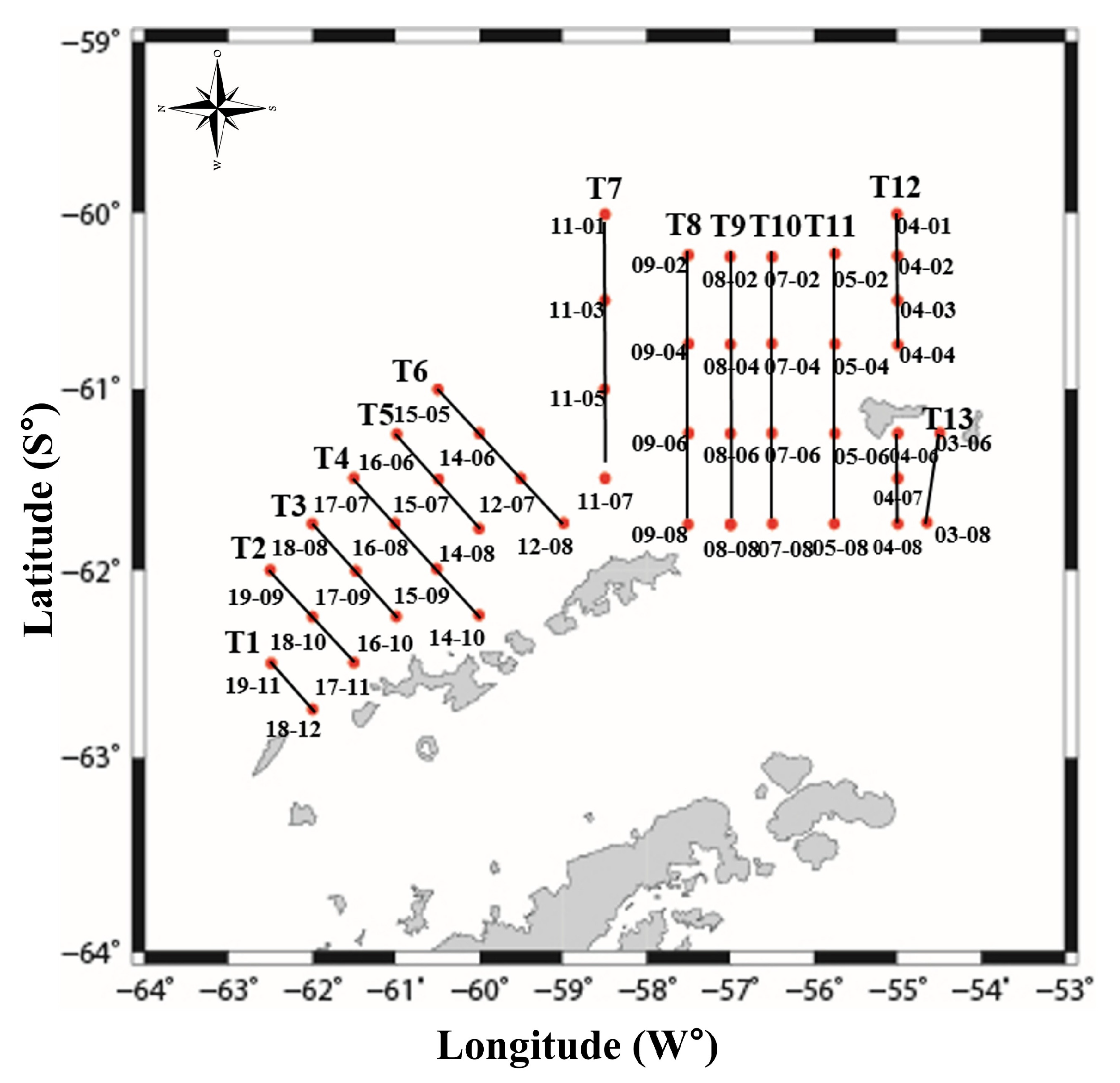
The survey area was located to the north of South Shetland Island and around Elephant Island and consisted of coastal zones formed by the continental shelf within 200 m around the islands, a frontal zone where water masses of different properties meet, and an offshore zone with increasing water depths. The survey was conducted during 8–15 March 2019, using the commercial vessel Kwangja-ho (3012 tonnage, Insung, Seoul, Republic of Korea). The acoustic survey was conducted at 14 survey transects and 48 trawl stations. The survey area covered a total of 18,579 km2 for transects T1–6 near South Shetland Island and 39,194 km2 for transects T7–13 near Elephant Island, totaling 57,773 km2 (Figure 1). The acoustic survey was conducted at a ship speed of approximately ~10 knots, while trawling maintained a towing speed of approximately 2–3 knots.
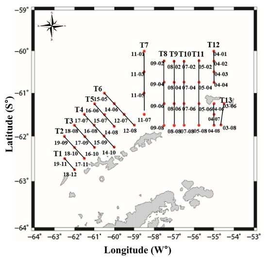
Figure 1.
Acoustic survey transects (solid lines) and trawl sampling stations (circles) for estimating krill density.
2.2. Acoustic System Configuration and Data Collection
The acoustic survey system consisted of an echosounder (EK60, Simrad, Kongsberg, Norway) with frequencies of 38 and 120 kHz (split-beam) attached to the Kwangja-ho’s hull, and the parameters of the echosounder were set according to the acoustic survey criteria proposed by the CCAMLR Scientific Committee (Table 1). The scientific fish finder was calibrated using a tungsten calibration sphere with a diameter of 38.1 mm before the acoustic survey, following the method described by Foote et al. [12]. The results of the system calibration are shown in Table 2.

Table 1.
Acoustic settings for the echosounder to collect acoustic data.
Table 2.
System calibration results for frequencies of 38 and 120 kHz.
2.3. Krill Sampling
Krill were collected using a midwater trawl used on commercial fishing vessels. The midwater trawl had a total net length of 167.6 m, mesh size of 15 mm, mouth height of 40 m, and width of 72 m. After capturing the organisms, the species from the trawl samples were identified and the total catch based on species was measured. Additionally, the fish collected at each station were frozen in an ultra-low temperature freezer aboard the Kwangja-ho vessel, along with seawater, in accordance with CCAMLR recommendations and transported to the National Institute of Fisheries Science. The “Discovery” measurement method, as suggested in the CCAMLR report [13], was used for measuring the body length of krill sampled at stations where krill were collected. In total, 150 krill specimens from each station were randomly selected and the length from the tip of the antennae to the tail, excluding the tail tip, at 1-mm intervals was measured. Weights were measured with 0.1 g accuracy using an electronic balance.
2.4. Acoustic Data Analysis
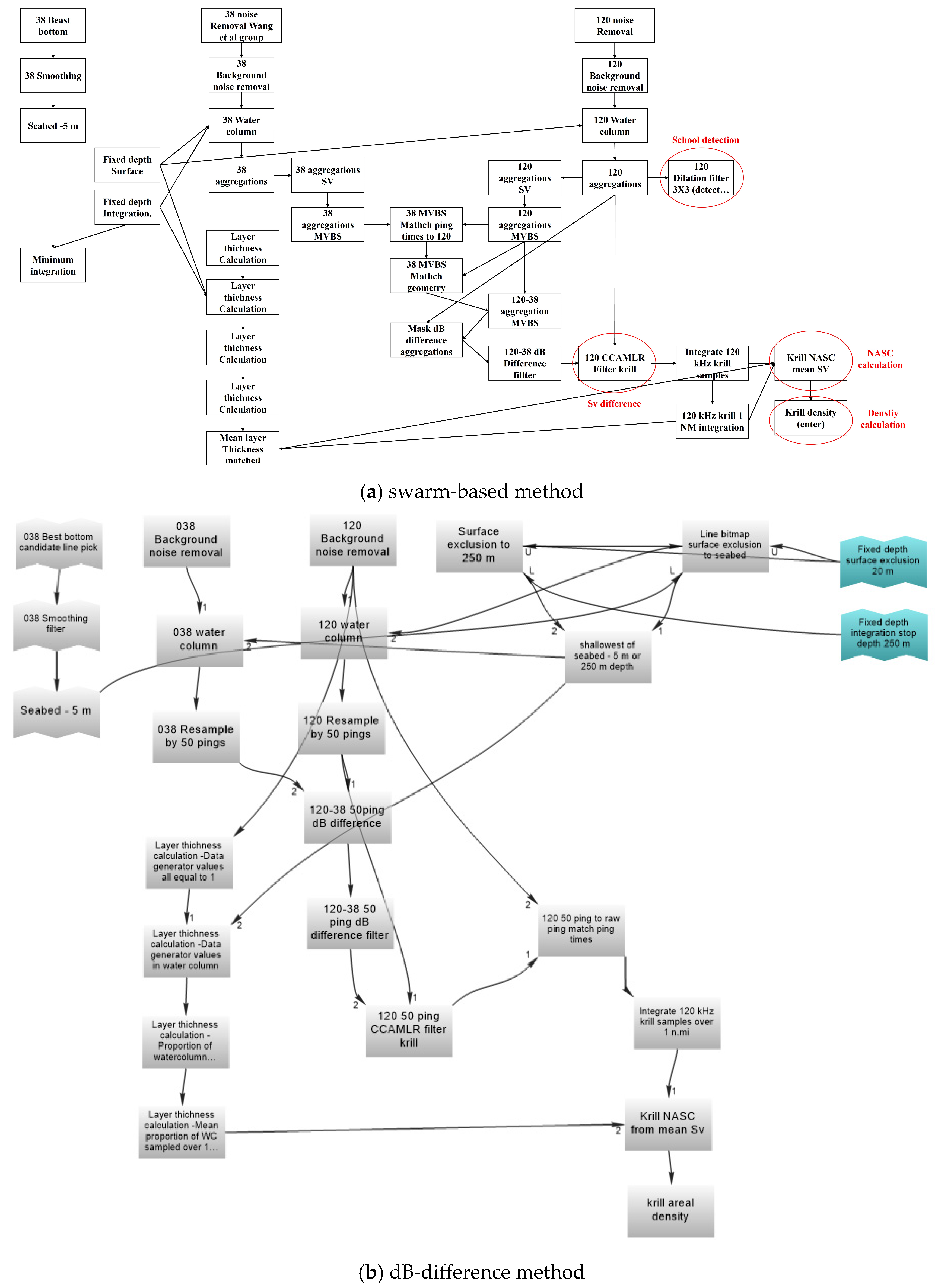
The acoustic data collected during the acoustic survey were analyzed using acoustic post-processing software (Echoview V 9.0, Echoview Software Pty Ltd., Hobart, Australia). To eliminate noise from ship-generated noise and electrical signals, we applied background noise removal functions and the method described by Wang et al. [14]. The flow chart of the noise and data processing process are shown in Figure 2. In the study area, which was a deep-water region with a depth of >1000 m, background noise occurred as the water depth increased. The time-varying threshold method was applied to remove it. This method involved artificially creating background noise and then subtracting it from the raw data. The parameter values for removing background noise are shown in Table 3.
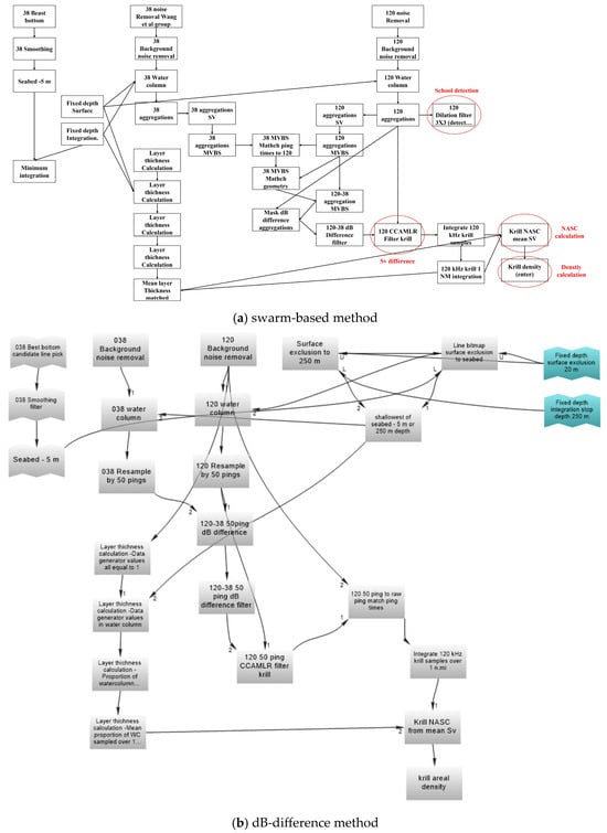
Figure 2.
Flowchart of acoustic data processing for (a) swarm-based method and (b) dB-difference method to assess krill density [14].
Table 3.
Parameters to remove background noise.
To remove the residual noise remaining even after subtracting the background noise, the function of a secondary data range bitmap was applied to eliminate noise smaller than the minimum SV (Volume backscatter, dB re 1 m−1) of krill and larger than the maximum SV [15]. Here, the data range bitmap set the krill to true, and all other values were treated as false. Following the above process, most of the noise was removed. However, to eliminate any remaining noise, an erosion filter with a 3 × 3 kernel was applied. The 3 × 3 represents the cell’s range, and it changed the value to the minimum value of the surrounding cell data. As the noise in the surrounding cells had a value of −999 dB, the noise disappeared. Although this denoising process removed all the noise, it weakened the echo and distorted the echo’s shape into empty spaces that were originally present. To recover from this phenomenon, the dilation filter function, which changed the value to the maximum value of the surrounding cell data, was used to fill the disappeared echo’s empty spaces. The ranges of cells of 5 × 5 and 7 × 7 were consecutively applied to fill in the empty spaces in the echo. Then, the echogram with the dilation filter 7 × 7 function was applied to the data range bitmap function and the krill’s SV range to create a mask. Finally, after using median 7 × 7, which functions to change values to the median of the surrounding cell material, the select operator was used to remove the echoes and noise selected by the previous mask and median 7 × 7, resulting in the denoised SV. After generating a data range bitmap that set the range of the krill in the echogram, the noise was completely removed upon selection, and the echo of the krill was obtained. The density of krill was analyzed using two methods: swarm-based and dB-difference methods.
- (1)
- Swarm-based analysis method
The processing and analysis of acoustic data are the basis for estimating the abundance of Antarctic krill. Among the current methods for obtaining the density of Antarctic krill, the swarm-based method is a data processing method proposed by [9] in SG-ASAM-17/02 in 2017 that involves using the “detect schools” function of acoustic data analysis software to extract krill schools. CCAMLR’s acoustic data processing method relies on the use of frequency differences at 38, 120, and 200 kHz to identify species and is based on a grid integration method of 50 ping × 5 m. The grid method has the disadvantage of noise elimination before estimating the density of krill, and it takes substantial time to process the data. Conversely, the swarm-based method has the advantage of reducing the data processing time by half compared with the dB-difference method. Because krill travel in swarms, research using swarm-based methods is being presented by the CCAMLR Science Committee.
To extract krill schools, the “detect schools” function of the acoustic data analysis software (Echoview V 9.0) was used, and the parameters in Table 4 were entered to extract schools that fit these parameters at a frequency of 120 kHz. The parameters in Table 3 were based on the research methodology proposed by Cox. After extracting the krill schools, the echoes of krill were extracted by setting the range of frequency difference at 120–38 kHz, and the 1 n.mile area scattering coefficient of the extracted krill was converted to density (Figure 2a).
Table 4.
Parameter settings for detecting krill families.
- (2)
- dB-difference analysis method
The dB-difference method applies a range of frequency differences of 120–38 kHz by integrating the cells at 50 ping × 5 m intervals, extracting the krill echoes contributing to 120 kHz and determining the density of krill with an area scattering coefficient of 1 n.mile (Figure 2b). Following the recommendations of the CCAMLR’s Scientific Committee, the acoustic data were denoised [15] and then analyzed down to a depth of 250 m, with a sea line from the surface to a depth of 20 m and a bottom line 5 m above the sea floor, considering the frequency detection distance [11].
2.5. Frequency Difference and Krill Echo Extraction Method
To extract the echo of the krill, it is necessary to understand the differences and characteristics of the krill’s frequencies at 38 and 120 kHz, and thus, the species can be clearly understood. Here, the frequency difference represents the difference in mean volume backscattering strength (MVBS) across multiple frequencies, and ∆MVBS was calculated by comparing the frequency-specific target strength (TS) of the target species to be separated and subtracting the frequency with the larger TS from the frequency with the smaller TS for achieving a positive value. Typically, for zooplanktons, they do not respond at 38 kHz but exhibit a strong response at 120 kHz. The new echograms at 38 and 120 kHz, matrixed in Equation (2), represent ∆MVBS.
The frequency discrimination range for identifying krill using acoustic data was determined based on the size of krill collected in the survey area (probability density function, PDF 95% range) [16,17]. In this study, we extracted krill density using two methods and compared the results. The first method applied the target strength (TS) to body length relationship derived from the SDWBA model across the size distribution of krill collected at the trawl apex. The second method used the dB-difference method to estimate krill size distributions along each acoustic survey line, with dB-difference ranging from −0.35 to 13.87 dB and −0.4 to 9.51 dB, respectively.
2.6. Estimation of the Density of Antartic Krill with Acoustic Data
To estimate the density of krill using acoustic data, we used the nautical area scattering coefficient (NASC) values converted from volume backscattering strength (SV) data obtained at a distance of one nautical mile from the echosounder. Equation (3) shows the conversion relationship from SV to NASC.
The NASC value represents the linear combination of signals received from aquatic organisms within a particular volume. Thus, the density ( g/m2) of the target organism can be obtained by dividing the average NASC value by the TS of the target fish (Equation (4)). The TS and backscattering cross-section () based on the target organism’s body length (L, mm) can be expressed by Equations (5) and (6), respectively.
Equation (7) indicates the relationship between the body length (L, cm)-weight (w, g) of the target organism.
The target organism’s density () can be calculated by dividing the average NASC within a one nautical mile volume by the backscattering cross-section () and multiplying by the weight (Equation (8)). All terms on the right side of Equation (8) except NASC are conversion factors (CF) for calculating the density from the acoustic data. These factors take into account the backscattering cross-section and body length–weight relationship of the target organism. Average values were used for both the backscattering cross-section and target organism’s weight.
The average target organism density () for the entire investigated sea area was the weighted mean of each transect’s average density data, as shown in Equation (9).
Here, : average density of the ith transect, EDSU of the ith transect, N: number of transects.
2.7. Marine Environmental Survey
In the 2019 survey, oceanographic data were collected at each station during Antarctic krill trawling to compare acoustic data from Antarctic waters with the oceanographic data, and CTDs (conductivity temperature depth, Seabird SBE-37, Seabird electronics, Bellevue, WA, USA) were used to measure water temperature and salinity variations across all stations.
3. Results
3.1. Catch Quantity and Krill Size Distribution
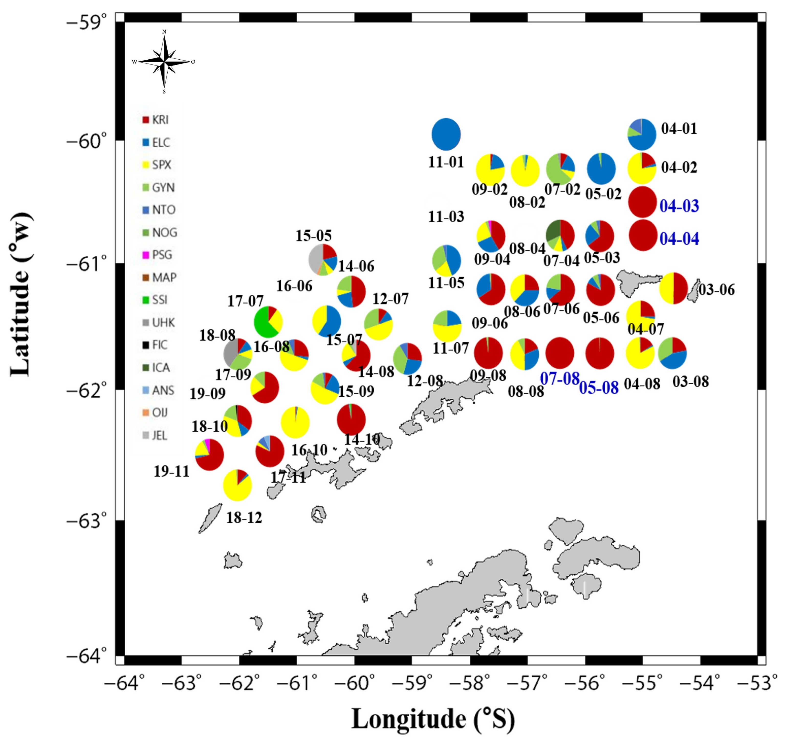
The results of the catch surveys conducted at a total of 48 stations in the survey area are presented in Table 5. Krill was most abundantly collected at station (St.) 04-04, amounting to 135 kg. The catch ratio of krill was >99% at St. 04-04, 04-03, 05-08, and 07-08 (Figure 3).
Table 5.
Trawl time, station, location, set time, depth, catch, and catch rate (KRI: Krill, Euphausia superba, ELC: Lanternfish, Electrona carlsbergi, GYN: Lanternfish, Gymnoscopelus nicholsi, ICA: Southern driftfish, Icichthys australis, NOG: Humped rockcod, Notothenia gibberifrons, NTO: Antarctic jonasfish, Notolepis coatis, SPX: Salps, Salpidae, UHK: Smooth hooked squid, Moroteuthis knipovitchi, ANS: Antarctic silverfish, Pleuragramma antarcticum, OIJ: Greater hooked squid, Moroteuthis ingens, JEL: Jellyfish, Medusae, SSI: Blackfin icefish, Chaenocephalus aceratus, PSG: Glacial squid, Psychroteuthis glacialis).

Figure 3.
Distribution of collected species according to trawl station (KRI: Krill, Euphausia superba, ELC: Lanternfish, Electrona carlsbergi, GYN: Lanternfish, Gymnoscopelus nicholsi, ICA: Southern driftfish, Icichthys australis, NOG: Humped rockcod, Notothenia gibberifrons, NTO: Antarctic jonasfish, Notolepis coatis, SPX: Salps, Salpidae, UHK: Smooth hooked squid, Moroteuthis knipovitchi, ANS: Antarctic silverfish, Pleuragramma antarcticum, OIJ: Greater hooked squid, Moroteuthis ingens, JEL: Jellyfish, Medusae, SSI: Blackfin icefish, Chaenocephalus aceratus, PSG: Glacial squid, Psychroteuthis glacialis).
Catch per unit effort (CPUE, kg/h) for krill was 52.1 kg/h at St 03-08, 289.0 kg/h at St. 04-04, 275.5 kg/h at St. 05-08, 178.6 kg/h at St. 09-08, and 264.5 kg/h at St. 14-10. In areas where the highest acoustic signals were observed, the target net haul was highest at 11,352.3 kg/h. In other areas, krill were either not captured or had CPUE values below 50 kg/h, with the highest krill capture occurring near Elephant Island.
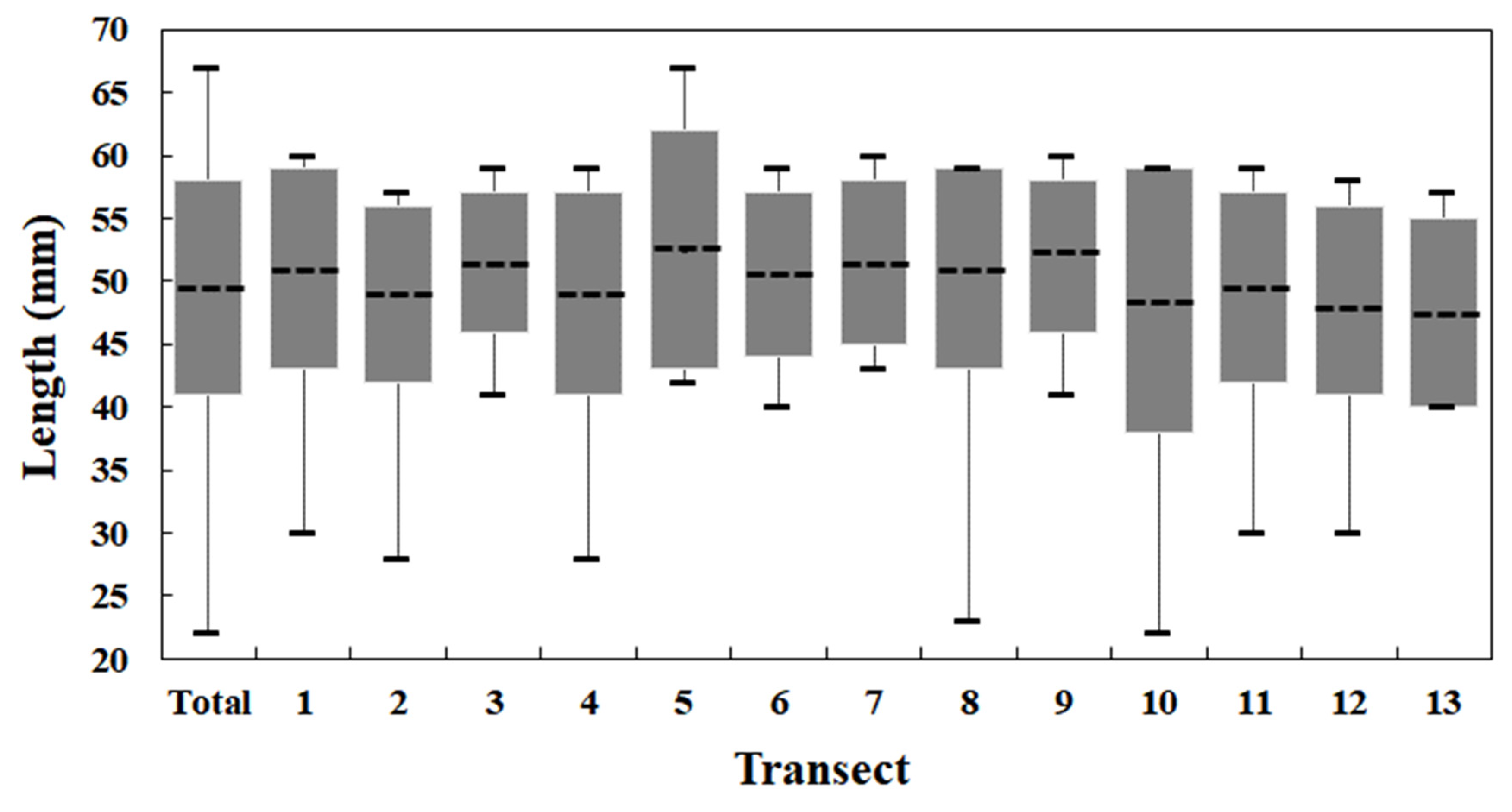
The length (L, mm) of krill caught in each transect was 30.0–60.0 mm (Avg. ± SD = 51.1 ± 4.1 mm) at T1, 28.0–57.0 mm (Avg. ± SD = 49.9 ± 3.6 mm) at T2, 41.0–59.0 mm (Avg. ± SD = 51.3 ± 2.7 mm) at T3, 28.0–59.0 mm (Avg. ± SD = 48.9 ± 3.9 mm) at T4, 42.0–67.0 mm (Avg. ± SD = 52.4 ± 4.6 mm) at T5, 40.0–59.0 mm (Avg. ± SD = 50.7 ± 3.1 mm) at T6, 43.0–60.0 mm (Avg. ± SD = 51.6 ± 3.3 mm) at T7, 23.0–59.0 mm (Avg. ± SD = 50.7 ± 4.1 mm) at T8, 41.0–60.0 mm (Avg. ± SD = 52.1 ± 3.2 mm) at T9, 22.0–59.0 mm (Avg. ± SD = 48.4 ± 5.5 mm) at T10, 30.0–59.0 mm (Avg. ± SD = 49.2 ± 3.7 mm) at T11, 30.0–58.0 mm (Avg. ± SD = 48.4 ± 3.9 mm) at T12, and 57.0–40.0 mm (Avg. ± SD = 47.7 ± 3.8 mm) at T13 (Figure 4). The length of krill caught at all stations ranged from 22.0 to 67.0 mm (Avg. ± SD = 49.06 ± 4.15 mm), and the distribution characteristics exhibited a single mode with a maximum frequency at 50 mm.
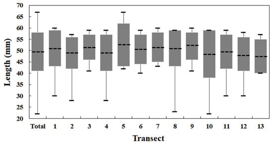
Figure 4.
Box plot of the size distribution of krill caught at all stations and transects. Krill size was defined as the interval containing at least 95% of the PDF of the krill size per transect, as in CCAMLR’s method. Boxes represent 95% of the krill size PDF, dashed lines represent the average value, and bars represent the minimum and maximum values.
3.2. Krill Distribution
- (1)
- Swarm-based method
Table 6 presents the krill density per transect estimated using the swarm-based analysis method. These estimates are based on the difference between 120 and 38 kHz frequencies, with two approaches: one using a standard total body mass for krill and another adjusted according to the actual krill size data collected at each transect. Using the standard body mass, the maximum weighted areal krill density was 82.97 g/m2, with a variance of 3986.72. When krill size data were incorporated, the estimated density decreased to 48.15 g/m2, with a reduced variance of 2262.92.
Table 6.
Density of krill determined using the swarm-based method with a difference in frequency between 120 and 38 kHz, based on the size of krill collected at all stations and per transect.
- (2)
- dB-difference method
Similarly, Table 7 shows the krill density estimates obtained using the dB-difference method. Following the same two approaches, the maximum weighted areal density was 56.83 g/m2 (variance: 1804.88) when using the standard krill body mass and 36.50 g/m2 (variance: 1275.67) when using size-specific data collected per transect.
Table 7.
Density of krill determined using the difference between the frequencies 120 and 38 kHz, based on krill size collected on all stations and on each transect using the dB-difference method.
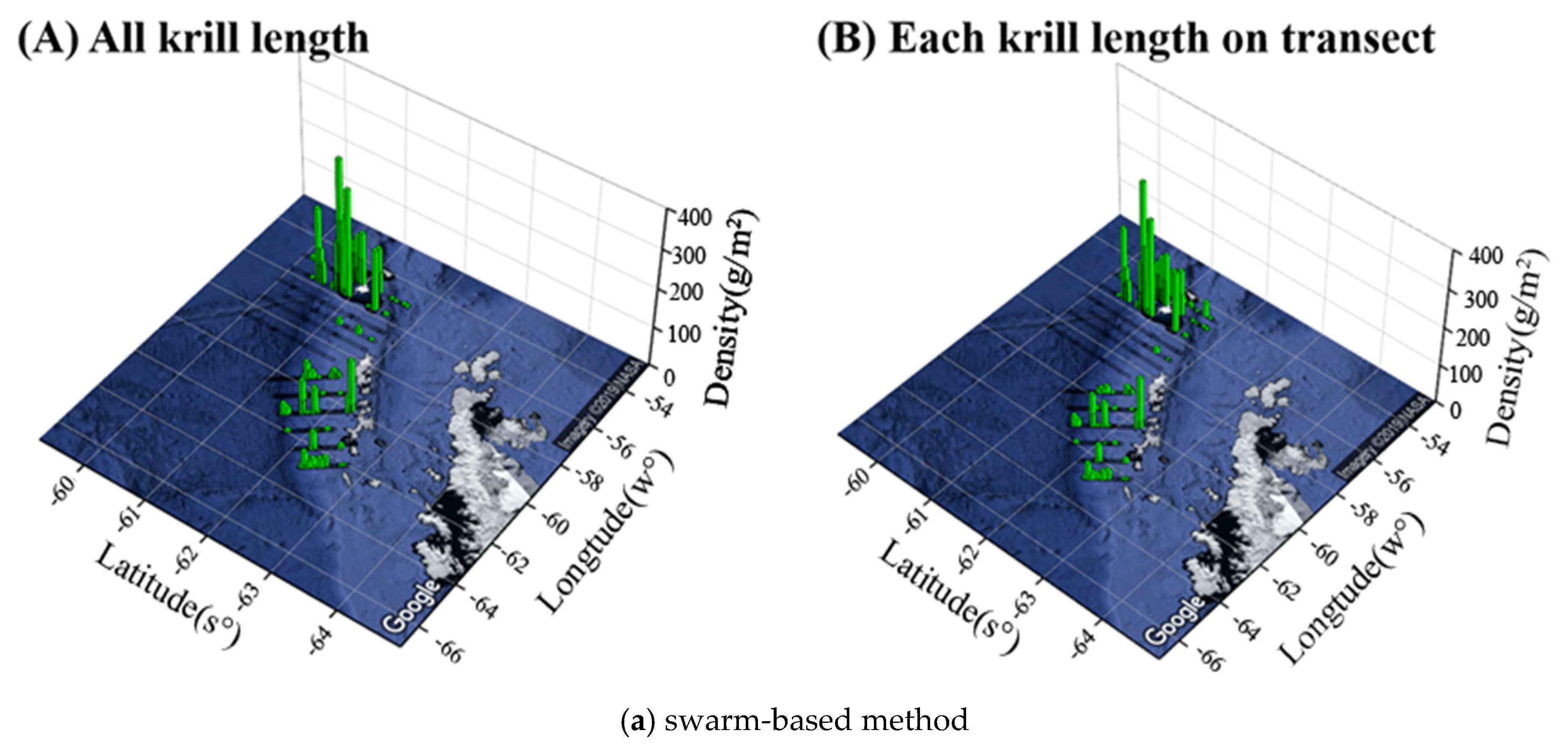
In this study, the distributions of krill densities determined using the swarm-based and dB-difference methods with frequency differences based on the total number of krill and the krill size collected per transect are shown in Figure 5. Krill density appeared higher near Elephant Island than in South Shetland Island, especially between transects 11 and 12 near the coast of Elephant Island.

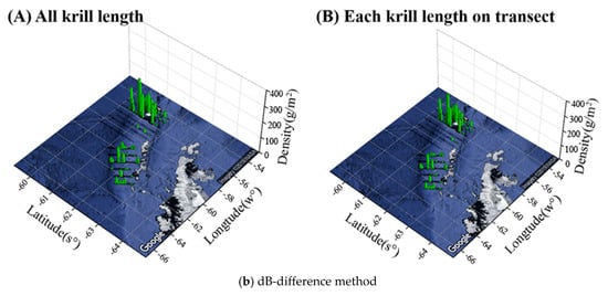
Figure 5.
Distribution of krill densities determined using the swarm-based and dB-difference methods with a difference between the frequencies 120 and 38 kHz, based on the total number of krill and the krill size collected per transect.
3.3. Krill Density
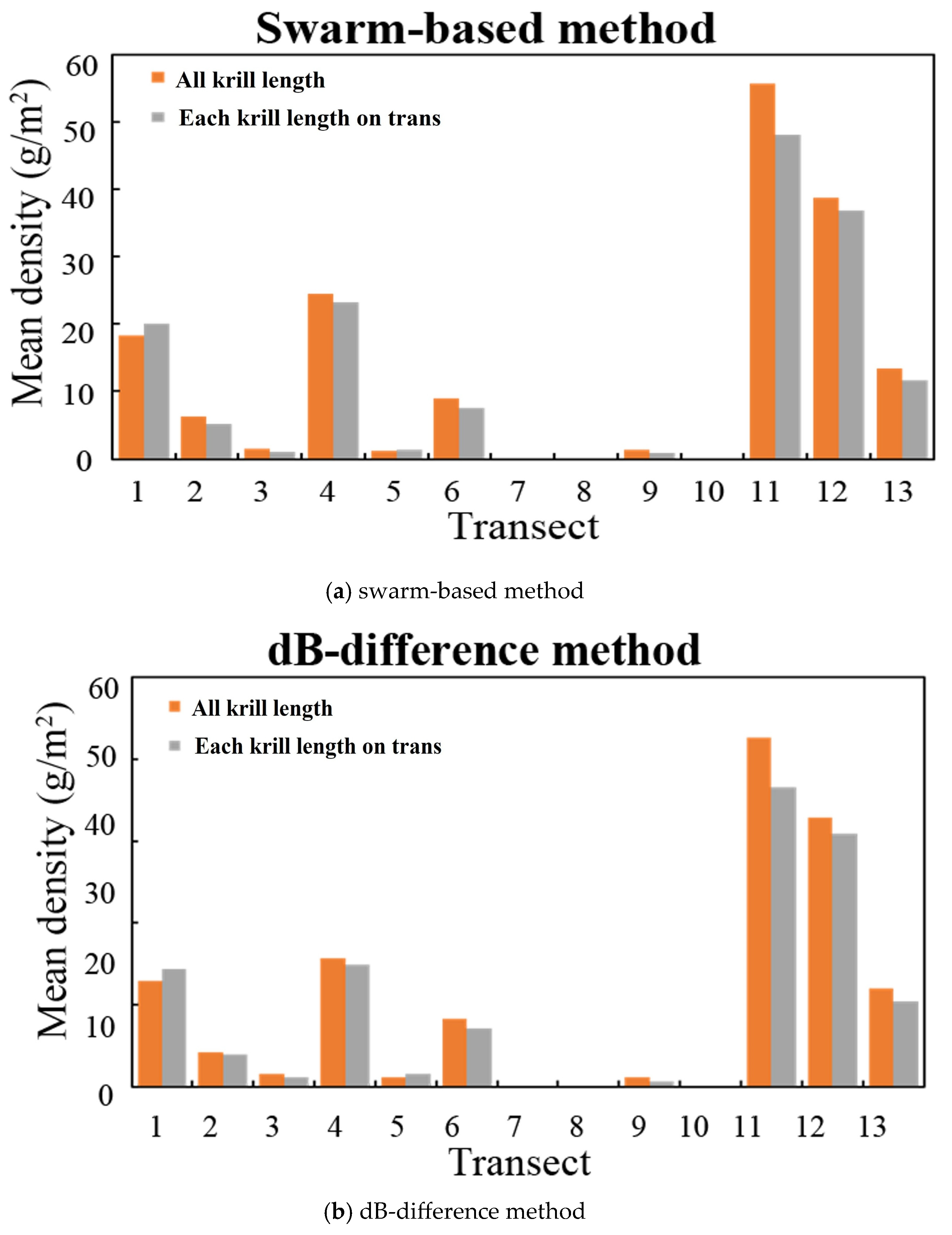
The average density of krill per transect with frequency difference based on krill size collected for all stations and transects using the swarm-based and dB-difference methods is shown in Figure 6. The density of krill was highest at T11 and T12 near Elephant Island, while T3, 5, 7, 8, 9, and 10 had low values of about ≤1 g/m2.
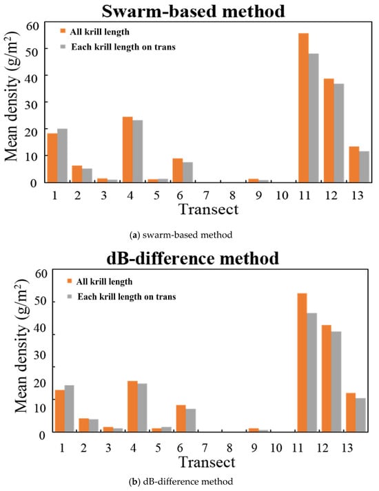
Figure 6.
(a) Average krill density per transect determined using the swarm-based method and (b) dB-difference method, based on krill size collected for all stations and transects with a frequency difference of 120 and 38 kHz.
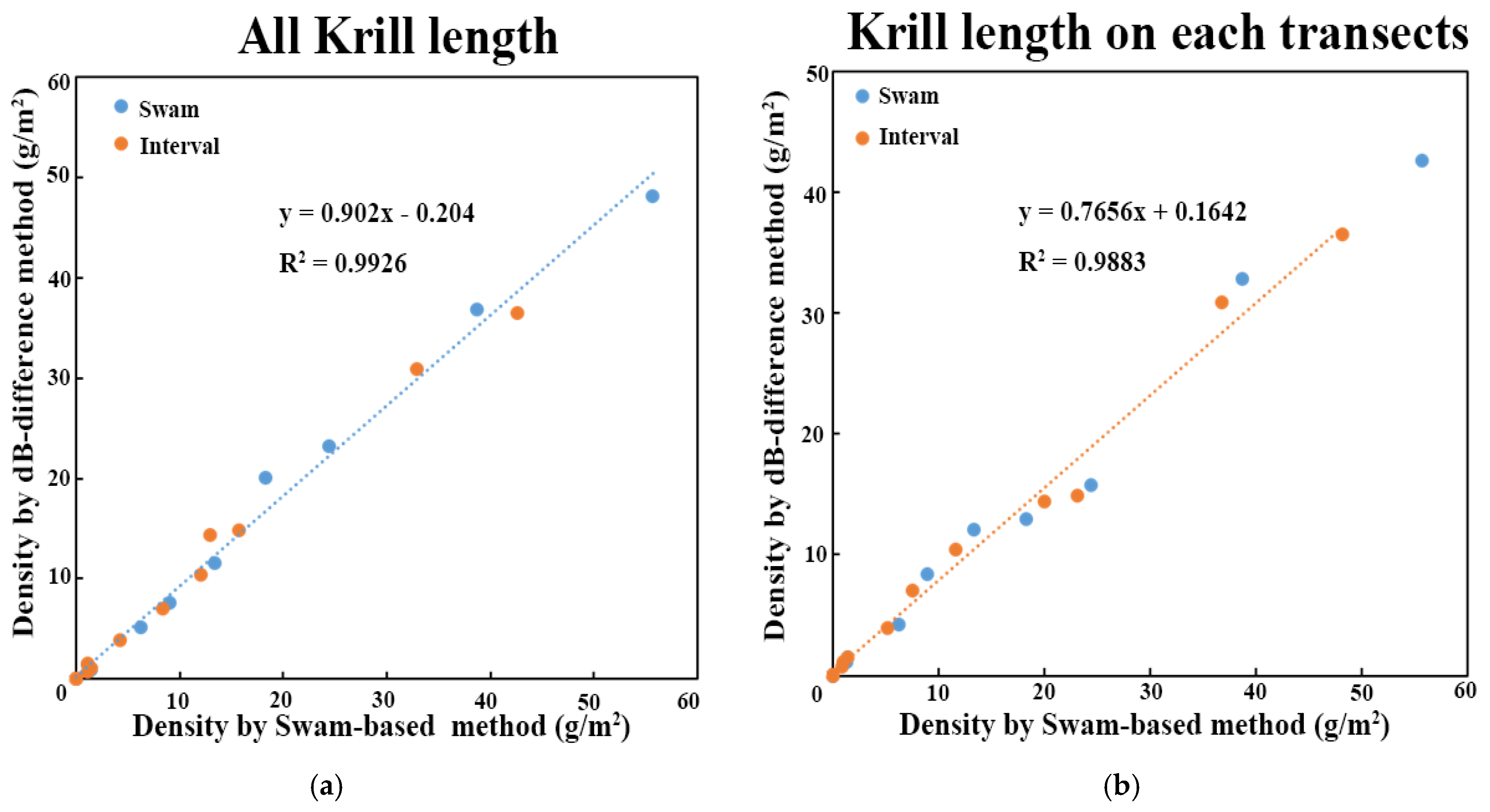
Using the swarm-based and dB-difference methods, a paired-samples t-test was performed to determine the correlation of the mean density of krill per transect by applying a difference in frequency of 120 and 38 kHz based on the krill size collected from all stations and transects. The results revealed a significant difference (p < 0.05) between the swarm-based and dB-difference methods based on the krill size collected from all stations; however, no significant difference (p > 0.05) was observed based on the krill size collected from each transect.
Using the swarm-based method across the entire survey area, based on the krill size collected from all stations and transects, the mean densities of krill collected per transect upon applying frequency differences were 14.86 g/m2 (coefficient of variation [CV] = 47.09%) and 13.10 g/m2 (CV = 41.16%), respectively. Furthermore, using the dB-difference method to apply frequency differences based on the krill size collected from all stations and transects, the mean densities of krill collected per transect were estimated to be 10.76 g/m2 (CV = 43.83%) and 10.14 g/m2 (CV = 53.48%), respectively (Figure 7).
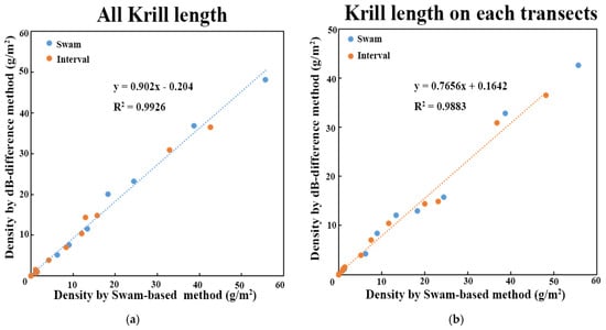
Figure 7.
(a) Correlation of mean krill density per transect determined using the swarm-based method and (b) dB-difference method, based on krill size collected for all stations and transects with a frequency difference of 120 and 38 kHz.
3.4. Marine Environmental Data Results
The vertical distribution of average temperature and salinity observed at all stations during the Antarctic krill trawl survey is presented in Figure 8. Water temperatures ranged 0.5–1.6 °C, decreasing to 1.1 °C at a depth of 50 m, with a low of 0.5 °C at 100 m, and increasing with depth. Salinity ranged 32.9–34.4 psu, with depth salinity increasing toward the bottom.
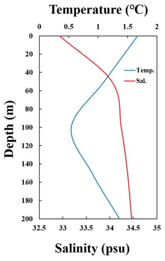
Figure 8.
Vertical distribution of the mean temperature (°C) and mean salinity (psu) at survey stations.
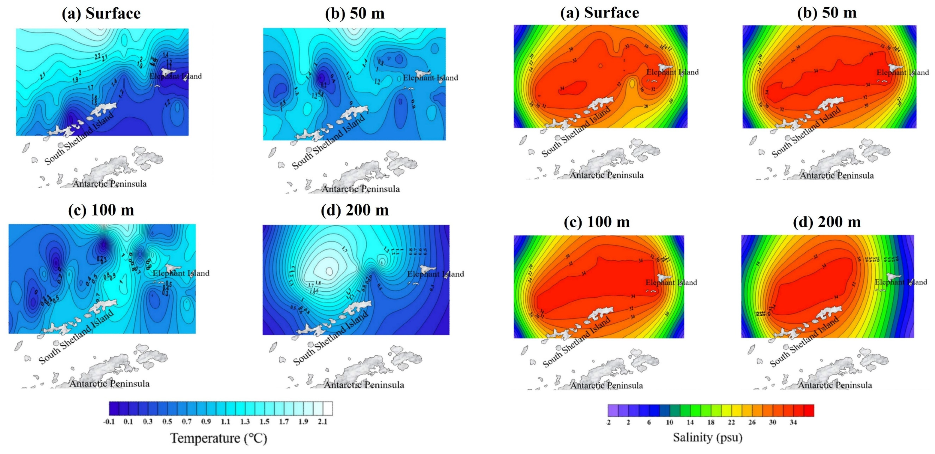
A horizontal distribution of water temperature and salinity was observed during the Antarctic krill sampling survey, from the surface to a depth of 200 m (Figure 9). The horizontal temperature distribution showed higher temperatures near the north of South Shetland Island and lower temperatures near the southeast and Elephant Island. Between depths of 50 and 100 m, temperatures were higher near the north and Elephant Island, contrasting with the surface layer, while temperatures decreased in the same areas from around 150 m. Salinity showed average values of 33.4 psu in the surface layer to 50-m depth, then consistently averaged at 34.3 psu beyond a 50-m depth.

Figure 9.
Vertical profiles of temperature and salinity in the survey area; (a) Surface, (b) 50 m, (c) 100 m, (d) 200 m.
4. Discussion
The length of Antarctic krill collected in this study ranged from 22.0 mm to 65.0 mm. The trawl nets used by the fishing vessels differed from conventional trawl nets. They consisted of an outer and inner net, with the inner net designed to allow only a certain size range of krill to be caught, minimizing the capture of small, juvenile krill. For future studies, using zooplankton nets, MOCNESS sampling devices, or similar equipment is recommended to clarify the size distribution and collect krill samples of various body sizes, including juveniles. This would improve the reliability of the study in terms of species identification and body size distribution.
Hydroacoustics utilizes frequency differences to distinguish Antarctic krill from other organisms. Krill and fish generally exhibit distinct frequency characteristics. Azzali et al. [18] reported a frequency difference range of −21.27 dB < ∆MVBS200-38 kHz < 5.77 dB for Antarctic krill. Sato et al. [19] applied a frequency difference interval of 2 dB < ∆MVBS200-38 kHz < 30 dB to identify zooplankton such as Euphausia pacifica and copepods similar to Antarctic krill. Additionally, Watkins et al. [20] reported that in Antarctic marine communities, where Antarctic krill comprise >90% of the community, the frequency difference interval does not exceed 2 dB < ∆MVBS120-38 kHz < 12 dB. Similarly, Reiss et al. [21] conducted acoustic surveys using scientific fish finders from 1996 to 2006 and reported a frequency difference range of 2.5 dB < ∆MVBS120-38 kHz < 14.7 dB for Antarctic krill with a body length range of 25–61 mm. Jarvis et al. [4] found similar results, with a frequency difference range of 2.5 dB < ∆MVBS120-38 kHz < 14.7 dB for krill measuring 20–60 mm. In contrast, Cox et al. [9] reported a frequency difference range of 3.4 dB < ∆MVBS120-38 kHz < 12.0 dB over a body length range of 21–61 mm for Antarctic krill. Overall, the range of frequency differences observed in this study aligns with previous findings. The difference range in the frequency applied depends on the krill body size; therefore, clear understanding of the krill body size distribution in the field is essential.
The annual distribution of Antarctic krill reported in previous studies showed a predominant distribution near the coasts of South Shetland Island and Elephant Island, with a higher density near Elephant Island than in other areas. This phenomenon is attributed to the formation of eddies near Elephant Island, which cause krill aggregations and along ocean currents [22]. The distribution of krill in the same waters exhibits substantial variations in response to different environmental influences and fluctuates over a cycle of approximately four to five years [9,23]. Krill density estimation studies have been conducted in several countries and are performed annually, although there are differences between surveyed waters [24,25,26]. For South Shetland Island, Hewitt et al. [23] reported density estimates of 1.2–60.2 g/m2 from 1991 to 2002 using frequencies of 38, 120, and 200 kHz. In 1998, Kang et al. [22] reported densities of 17.00–40.19 g/m2 for Antarctic krill using a 38 kHz frequency. The density of Antarctic krill estimated at 200 kHz in 2006 was 22.37 g/m2, whereas other studies reported a density of 44.9 g/m2 at South Shetland Island in 2002 [9,24].
The CCAMLR conducts joint research annually on Antarctic krill resource management, primarily focusing on countries involved in krill harvesting. The design, planning, and implementation of acoustic krill stock assessment surveys were undertaken by CCAMLR-2000 in 1995, and the SG-ASAM has been in operation since 2011 [11]. In 2018, the CCAMLR Scientific Committee and General Assembly approved a large-scale Antarctic krill survey involving Australia, the United Kingdom, China, Ukraine, Norway, and South Korea, a nation engaged in krill harvesting. It included midwater trawl surveys at designated stations per transect. Krill trawlers operating in Antarctic waters for extended periods, can continuously retrieve acoustic data, offering a cost-effective and laborsaving alternative to research vessels [27,28].
5. Conclusions
Collecting and analyzing acoustic data of Antarctic krill using commercial vessels are commonly practiced in countries such as Chile, Norway, and South Korea. In this study, we estimated the density of Antarctic krill in the coastal waters of South Shetland Island and around Elephant Island using fish finders aboard commercial fishing vessels. Krill was most abundantly collected at station 04-04, amounting to 135 kg. The catch ratio of krill was >99% at St. 04-04, 04-03, 05-08, and 07-08. The size of krill caught at all stations ranged from 22.0 to 67.0 mm (Avg. ± SD = 49.06 ± 4.15 mm), and the distribution characteristics exhibited a single mode with a maximum frequency at 50 mm. Using the swarm-based method for the entire survey area, the mean densities of krill according to stations and transects, based on frequency differences according to krill size, were 14.86 g/m2 (coefficient of variation [CV] = 47.09%) and 13.10 g/m2 (CV = 41.16%), respectively. Furthermore, using the dB-difference method for the entire survey area, the average densities of krill according to stations and transects were estimated to be 10.76 g/m2 (CV = 43.83%) and 10.14 g/m2 (CV = 53.48%), respectively, using the frequency difference based on krill size determined at all stations and per transect. The Pearson correlation coefficient from t-tests conducted to assess the correlation based on tracking was 0.99, which was not statistically significant (p > 0.05). These results are expected to be useful for Antarctic krill resource management.
Author Contributions
Conceptualization, K.L.; methodology, I.H.; software, G.P.; validation, K.L.; formal analysis, G.P.; investigation, I.H. and S.C. (Seokgwan Choi).; resources, K.L.; data curation, I.H.; writing—original draft preparation, G.P.; writing—review and editing, G.P.; visualization, G.P.; supervision, K.L.; project administration, K.L.; funding acquisition, S.C. (Sangdeok Chung). All authors have read and agreed to the published version of the manuscript.
Funding
This work was supported by the National Institute of Fisheries Science, Korea (No. R2023001). This work was supported by the National Institute of Fisheries Science, Korea (No. R2025003).
Data Availability Statement
The original contributions presented in this study are included in the article. Further inquiries can be directed to the corresponding author.
Acknowledgments
This work was supported by the National Institute of Fisheries Science, Korea (No. R2025003).
Conflicts of Interest
The authors declare no conflict of interest.
References
- Hewitt, R.; Demer, D.A. Dispersion and abundance of Antarctic krill in the vicinity of Elephant Island in the 1992 austral summer. Mar. Ecol. Prog. Ser. 1993, 99, 29–39. [Google Scholar] [CrossRef]
- Everson, I. Distribution and Standing, The Southern Ocean. Krill Biology, Ecology and Fisheries; Blackwell Science: Everson, Australia, 2000; pp. 63–79. [Google Scholar] [CrossRef]
- Atkinson, A.; Siegel, V.; Pakhomov, E.A.; Jessopp, M.J.; Loeb, V. A re-appraisal of the total biomass and annual production of Antarctic krill. Deep Sea Res. I Oceanogr. Res. Pap. 2009, 56, 727–740. [Google Scholar] [CrossRef]
- Jarvis, T.; Kelly, N.; Kawaguchi, S.; van Wijk, E.; Nicol, S. Acoustic characterisation of the broad-scale distribution and abundance of Antarctic krill (Euphausia superba) off East Antarctica (30–80° E) in January–March 2006. Deep Sea Res. II Top. Stud. Oceanogr. 2010, 57, 916–933. [Google Scholar] [CrossRef]
- Fielding, S.; Watkins, J.L.; Trathan, P.N.; Enderlein, P.; Waluda, C.M.; Stowasser, G.; Tarling, G.A.; Murphy, E.J. Interannual variability in Antarctic krill (Euphausia superba) density at South Georgia, Southern Ocean: 1997–2013. ICES J. Mar. Sci. 2014, 71, 2578–2588. [Google Scholar] [CrossRef]
- Hewitt, R.P.; Low, E.H.L. The fishery on Antarctic krill: Defining an ecosystem approach to management. Rev. Fish. Sci. 2000, 8, 235–298. [Google Scholar] [CrossRef]
- Hewitt, R.; Watkins, J.; Naganobu, M.; Sushin, V.; Brierley, A.; Demer, D.; Kasatkina, S.; Takao, Y.; Goss, C.; Malyshko, A. Biomass of Antarctic krill in the Scotia Sea in January/February 2000 and its use in revising an estimate of precautionary yield. Deep Sea Res. II Top. Stud. Oceanogr. 2004, 51, 1215–1236. [Google Scholar] [CrossRef]
- Lawson, G.L.; Wiebe, P.H.; Stanton, T.K.; Ashjian, C.J. Euphausiid distribution along the Western Antarctic Peninsula—Part A: Development of robust multi-frequency acoustic techniques to identify euphausiid aggregations and quantify euphausiid size, abundance, and biomass. Deep Sea Res. II Top. Stud. Oceanogr. 2008, 55, 412–431. [Google Scholar] [CrossRef]
- Cox, M.J.; Watkins, J.L.; Reid, K.; Brierley, A.S. Spatial and temporal variability in the structure of aggregations of Antarctic krill (Euphausia superba) around South Georgia, 1997–1999. ICES J. Mar. Sci. 2011, 68, 489–498. [Google Scholar] [CrossRef]
- La, H.S.; Lee, H.; Kang, D.; Lee, S.; Shin, H.C. Volume backscattering strength of ice krill (Euphausia crystallorophias) in the Amundsen Sea coastal polynya. Deep Sea Res. II 2016, 123, 86–91. [Google Scholar] [CrossRef]
- Fielding, S.; Cossio, A.; Cox, M.; Reiss, C.; Skaret, G.; Demer, D.; Watkins, J.; Zhao, X. A condensed history and document of the method used by CCAMLR to estimate krill biomass (B0) in 2010. In Proceedings of the CCAMLR WG-EMM, Bologna, Italy, 4–15 July 2016; Volume 16, p. 2010. [Google Scholar]
- Foote, K.G. Calibration of Acoustic Instruments for Fish Density Estimation: A Practical Guide 144; International Council for the Exploration of the Sea: København, Demark, 1987. [Google Scholar]
- CCAMLR (Commission for the Conservation of Antarctic Marine Living Resources). Scientific Observers Manual—2011. Observation Guidelines and Reference Material; CCAMLR: Hobart, Australia, 2011; p. 71. [Google Scholar]
- Wang, X.; Zhao, X.; Zhang, J. A noise removal algorithm for acoustic data with strong interference based on post-processing techniques. In Proceedings of the CCAMLR SG-ASAM, Busan, Republic of Korea, 9–13 March 2015; Volume 11. [Google Scholar]
- De Robertis, A.; Higginbottom, I. A post-processing technique to estimate the signal-to-noise ratio and remove echosounder background noise. ICES J. Mar. Sci. 2007, 64, 1282–1291. [Google Scholar] [CrossRef]
- CCAMLR (Commission for the Conservation of Antarctic Marine Living Resources). Report of the twenty-ninth meeting of the Scientific Committee. Hobart, Australia, Commission for the Conservation of Antarctic Marine Living Resources. In Proceedings of the SC-CAMLR-XXIX, Hobart, Australia, 25–29 October 2010; 426p. [Google Scholar]
- Fielding, S.; Watkins, J.; Cossio, A.; Reiss, C.; Watters, G.; Calise, L.; Skaret, G.; Takao, Y.; Zhao, X.; Agnew, D.; et al. The ASAM 2010 assessment of krill biomass for area 48 from the Scotia Sea. CCAMLR 2000 synoptic survey. In Proceedings of the CCAMLR WG-EMM, Busan, Republic of Korea, 11–22 July 2011; Volume 11. [Google Scholar]
- Azzali, M.; Leonori, I.; Lanciani, G. A hybrid approach to acoustic classification and length estimation of krill. CCAMLR Sci. 2004, 11, 33–58. [Google Scholar]
- Sato, M.; Horne, J.K.; Parker-Stetter, S.L.; Keister, J.E. Acoustic classification of coexisting taxa in a coastal ecosystem. Fish. Res. 2015, 172, 130–136. [Google Scholar] [CrossRef]
- Watkins, J. Verification of the acoustic techniques used to identify Antarctic krill. ICES J. Mar. Sci. 2002, 59, 1326–1336. [Google Scholar] [CrossRef]
- Reiss, C.S.; Cossio, A.M.; Loeb, V.; Demer, D.A. Variations in the biomass of Antarctic krill (Euphausia superba) around the South Shetland Islands, 1996–2006. ICES J. Mar. Sci. 2008, 65, 497–508. [Google Scholar] [CrossRef]
- Kang, D.; Hwang, D.; Kim, S. Biomass and distribution of Antarctic krill, Euphausia superba, in the northern part of the South Shetland Islands, Antarctic Ocean. Korean J. Fish. Aquat. Sci. 1999, 32, 737–747. [Google Scholar]
- Hewitt, R.P.; Demer, D.A.; Emery, J.H. An 8-year cycle in krill biomass density inferred from acoustic surveys conducted in the vicinity of the South Shetland Islands during the austral summers of 1991–1992 through 2001–2002. Aqua Living Resour. 2006, 16, 205–213. [Google Scholar] [CrossRef]
- Kang, D.H.; Shin, H.C.; Lee, Y.H.; Kim, Y.S.; Kim, S.A. Acoustic estimate of the krill (Euphausia superba) density between south Shetland islands and south Orkney islands, Antarctica, during 2002/2003 Austral summer. Ocean Polar Res. 2005, 27, 75–86, (In Korean with English Abstract). [Google Scholar]
- Choi, S.G.; Han, I.; Hwang, D.J.; Kim, T.H.; An, D.H.; Lee, K. Species identification of Antarctic krill Euphausia superba using the 2-frequency difference method. Korean J. Fish. Aquat. Sci. 2017, 50, 788–798. [Google Scholar]
- Choi, S.G.; Han, I.; An, D.H.; Chung, S.D.; Yoon, E.A.; Lee, K. Estimating the abundance of Antarctic krill Euphausia superba using a commercial trawl vessel. Korean J. Fish. Aquat. Sci. 2018, 51, 435–443. [Google Scholar]
- Krafft, B.A.; Skaret, G.; Knutsen, T. An Antarctic krill (Euphausia superba) hotspot: Population characteristics, abundance and vertical structure explored from a krill fishing vessel. Polar Biol. 2015, 38, 1687–1700. [Google Scholar] [CrossRef]
- Choi, S.G.; Lee, H.; Lee, K.; Lee, J. A study on calibration for commercial split beam echosounder using the bottom backscattering strength from a fishing vessel near the South Shetland Islands, Antarctica. J. Korean Soc. Fish. Technol. 2016, 52, 318–324. [Google Scholar] [CrossRef]


Disclaimer/Publisher’s Note: The statements, opinions and data contained in all publications are solely those of the individual author(s) and contributor(s) and not of MDPI and/or the editor(s). MDPI and/or the editor(s) disclaim responsibility for any injury to people or property resulting from any ideas, methods, instructions or products referred to in the content. |
© 2025 by the authors. Licensee MDPI, Basel, Switzerland. This article is an open access article distributed under the terms and conditions of the Creative Commons Attribution (CC BY) license (https://creativecommons.org/licenses/by/4.0/).