
Groundwater Vulnerability and Environmental Impact Assessment of Urban Underground Rail Transportation in Karst Region: Case Study of Modified COPK Method

 , and
, and
Abstract
1. Introduction
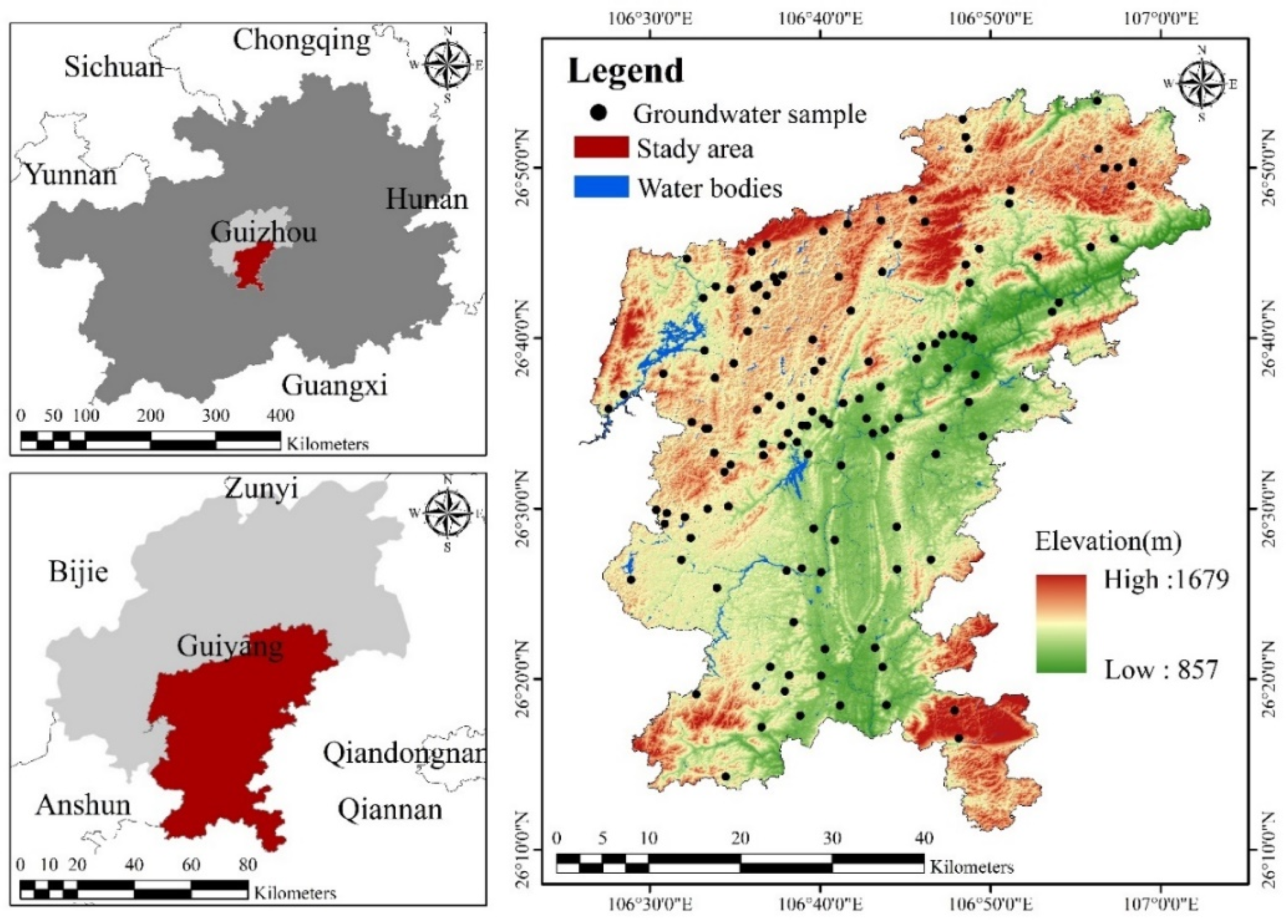
2. Study Area
3. Methodology
3.1. Data Source and Pre-Processing
3.2. COP Model
3.2.1. C Factor
3.2.2. O Factor
3.2.3. P Factor
3.3. Modified COPK Model
3.3.1. Modified C Factor
3.3.2. Modified O Factor
3.3.3. K Factor
3.4. Model Validation
3.5. Spatial Autocorrelation
3.6. Groundwater Risk Calculation
4. Results
4.1. GV Map
4.2. Model Validation Results
4.3. Spatial Autocorrelation Results
4.4. Groundwater Risk
5. Discussion
5.1. Effectiveness of the Modified COPK Model Under the Urbanization Context
5.2. Analysis of Groundwater Risk Assessment
5.3. Urban Planning and Infrastructure Development for Sustainable Groundwater Management
5.4. Limitations and Future Research
6. Conclusions
Author Contributions
Funding
Data Availability Statement
Acknowledgments
Conflicts of Interest
Appendix A. The Scoring Process of the Traditional COP Model

Appendix B. Karst Development Classification in DBJ52/T 099-2020

| K Levels | Carbonate Formation Types |
|---|---|
| Strong | Pure carbonate formations with wide exposure and substantial continuous thickness. |
| Moderate | Sub-pure carbonate formations, in which carbonate rocks are distributed in a banded pattern with a certain degree of continuity in thickness. |
| Low | Carbonate-poor formations which are characterized by interbedded carbonate layers with limited lateral continuity and thin single-layer thickness. |
| K Levels | Karst Development Features |
|---|---|
| Strong | Surface karst features such as depressions, sinkholes, and dolines are commonly observed, with dense distributions of solution grooves, solution troughs, and limestone pinnacles, and occasional occurrences of karst collapses. Subsurface soil cavities and solution caves are well developed. |
| Moderate | Surface karst features such as depressions, sinkholes, dolines, solution grooves, solution troughs, and limestone pinnacles are well developed, with occasional occurrences of small-scale karst collapses. Subsurface features such as soil cavities and solution caves are also relatively well developed |
| Low | Surface karst features are sparsely developed and mainly consist of solution grooves and solution troughs. Subsurface karst features are dominated by solution pores, crystal pores, and corrosion pitting, with no development of soil cavities |
| K Levels | Karst Development Features |
|---|---|
| Strong | Subsurface karst conduits or underground rivers are present, and springs are relatively abundant |
| Moderate | Small-scale subsurface karst conduits are present, and spring outcrops are relatively scarce |
| Low | Karst fractures are mostly filled, and spring outcrops are sparse or absent |
| K Levels | Karst Development Features |
|---|---|
| Strong |
|
| Moderate |
|
| Low |
|
Appendix C. Pollution Load Risk Index Calculation and Scoring Process
| Pollution Types | Toxicity Category | Scores | Buffer (km) | |
|---|---|---|---|---|
| Industrial pollution | Petroleum processing, coking, and nuclear fuel processing industries | 2.5 | 1.5 | |
| Non-ferrous metal smelting and rolling processing industry | 3 | 1 | ||
| Ferrous metal smelting and rolling processing industry | 2 | 1 | ||
| Manufacturing of chemical raw materials and chemical products | 2.5 | 2 | ||
| Textile industry | 1 | 2 | ||
| Leather, fur, feather (down), and related products industry | 1 | 2 | ||
| Metal products industry | 1.5 | 1 | ||
| Other industries | 0.2 | 1 | ||
| Mining activities | Coal mining and washing industry, and oil and natural gas extraction industry | 1.5 | 1.5 | |
| Ferrous metal mining and dressing industry | 2 | 1 | ||
| Non-ferrous metal mining and dressing industry | 3 | 1 | ||
| Non-metallic mineral mining and dressing industry | 1 | 1 | ||
| Hazardous waste disposal sites | Mainly industrial hazardous waste and hazardous chemicals | 2 | 1 | |
| Landfills | Mainly domestic waste | 1.5 | 2 | |
| Gas stations | Petroleum hydrocarbons and polycyclic aromatic hydrocarbons (PAHs) | 2.5 | 1.5 | |
| Agricultural pollution | Cultivation | Chemical fertilizers, pesticides, and heavy metals | 1.5 | 1.5 |
| Farming | Antibiotics | 1 | 1 | |
| Golf courses | Pesticides | Industrial, domestic, and agricultural wastewater discharges | 1.5 | 1.5 |
| Pollution Types | Release Probability | Scores | |
|---|---|---|---|
| Industrial pollution | Commissioned after 2011 | 0.2 | |
| Commissioned between 1998 and 2011 | 0.6 | ||
| Commissioned before 1998 or without protective measures | 1 | ||
| Mining activities | Closed, with mine shafts backfilled | 0.5 | |
| Closed, with mine shafts not backfilled | 0.7 | ||
| In operation | 0.3 | ||
| Tailings pond or transfer stations equipped with anti-seepage measures | 0.5 | ||
| Tailings ponds or transfer stations without anti-seepage measures | 1 | ||
| Landfills | ≤5 years, harmless rating AAA | 0.1 | |
| >5 years, harmless rating AAA | 0.2 | ||
| ≤5 years, harmless rating AA | 0.2 | ||
| >5 years, harmless rating AA | 0.4 | ||
| ≤5 years, harmless rating A | 0.4 | ||
| >5 years, harmless rating A | 0.5 | ||
| Basic protection, harmless rating B | 0.6 | ||
| No protection, harmless rating B | 1 | ||
| Hazardous waste disposal sites | Regulated | 0.1 | |
| Without protective measures | 1 | ||
| Gas stations | ≤5 years, with double-layer tanks or anti-seepage basins | 0.1 | |
| (5, 15] years, with double-layer tanks or anti-seepage basins | 0.2 | ||
| >15 years, with double-layer tanks or anti-seepage basins | 0.5 | ||
| ≤5 years, with single-layer tanks and without anti-seepage basins | 0.2 | ||
| (5, 15] years, with single-layer tanks and without anti-seepage basins | 0.6 | ||
| >15 years, with single-layer tanks and without anti-seepage basins | 1 | ||
| Agricultural pollution | Agricultural cultivation | Paddy field | 0.3 |
| Dry land | 0.7 | ||
| Large-scale livestock farms | With protective measures | 0.3 | |
| Without protective measures | 1 | ||
| Golf courses | ≤18 holes | 0.1 | |
| (18, 36] holes | 0.2 | ||
| >18 holes | 0.5 | ||
| Pollution Types | Type | Scores | |
|---|---|---|---|
| Industrial pollution (Wastewater discharge volume, unit: ×103 t/a) | ≤1 | 1 | |
| (1, 5] | 2 | ||
| (5, 10] | 4 | ||
| (10, 50] | 6 | ||
| (50, 100] | 8 | ||
| (100, 500] | 9 | ||
| (500, 1000] | 10 | ||
| >1000 | 12 | ||
| Mining activities (Scale, unit: dimensionless) | Small scale | 3 | |
| Medium scale | 6 | ||
| Large scale | 9 | ||
| Landfills (Filling volume, unit: ×103 m3) | ≤1000 | 4 | |
| (1000, 5000] | 7 | ||
| >5000 | 9 | ||
| Hazardous waste disposal sites (Landfilled volume, unit: ×103 m3) | ≤10 | 4 | |
| (10, 50] | 7 | ||
| >50 | 9 | ||
| Gas stations (Number of 30 m3 fuel tanks, unit: units) | 1 | 1 | |
| Agricultural pollution | Cultivation (Fertilizer application, unit: kg/ha) | ≤180 | 1 |
| (180, 225] | 3 | ||
| (225, 400] | 5 | ||
| >400 | 7 | ||
| Large-scale livestock farms (COD discharge, unit: t/a) | ≤2 | 1 | |
| (2, 10] | 2 | ||
| (10, 50] | 4 | ||
| (50, 100] | 6 | ||
| (100, 150] | 8 | ||
| (150, 200] | 9 | ||
| >200 | 10 | ||
| Golf courses (Area occupied, unit: hm2) | ≤100 | 1 | |
| (100, 1000] | 3 | ||
| (1000, 5000] | 5 | ||
| (5000, 10,000] | 7 | ||
| >10,000 | 9 | ||
References
- Çallı, K.Ö.; Chiogna, G.; Bittner, D.; Sivelle, V.; Labat, D.; Richieri, B.; Çalli, S.S.; Hartmann, A. Karst water resources in a changing world: Review of solute transport modelling approaches. Rev. Geophys. 2025, 63, e2023RG000811. [Google Scholar] [CrossRef]
- Reberski, J.L.; Terzić, J.; Maurice, L.D.; Lapworth, D.J. Emerging organic contaminants in karst groundwater: A global level assessment. J. Hydrol. 2022, 604, 127242. [Google Scholar] [CrossRef]
- Guo, F.; Yang, J.; Li, H.; Li, G.; Zhang, Z. A convLSTM conjunction model for groundwater level forecasting in a karst aquifer considering connectivity characteristics. Water 2021, 13, 2759. [Google Scholar] [CrossRef]
- Jiang, X.; Lei, M.; Zhao, H. Review of the advanced monitoring technology of groundwater–air pressure (enclosed potentiometric) for karst collapse studies. Environ. Earth Sci. 2019, 78, 701. [Google Scholar] [CrossRef]
- Wang, Z.-J.; Yue, F.-J.; Lu, J.; Wang, Y.-C.; Qin, C.-Q.; Ding, H.; Xue, L.-L.; Li, S.-L. New insight into the response and transport of nitrate in karst groundwater to rainfall events. Sci. Total Environ. 2022, 818, 151727. [Google Scholar] [CrossRef]
- Jiang, C.; Jourde, H.; Aliouache, M.; Wang, X. The effect of seasonal variation of precipitation/recharge on karst genesis behaviors in different climatic contexts. J. Hydrol. 2023, 626, 130385. [Google Scholar] [CrossRef]
- Siarkos, I.; Sevastas, S.; Mallios, Z.; Theodossiou, N.; Ifadis, I. Investigating groundwater vulnerability variation under future abstraction scenarios to estimate optimal pumping reduction rates. J. Hydrol. 2021, 598, 126297. [Google Scholar] [CrossRef]
- Xiong, H.; Wang, Y.; Guo, X.; Han, J.; Ma, C.; Zhang, X. Current status and future challenges of groundwater vulnerability assessment: A bibliometric analysis. J. Hydrol. 2022, 615, 128694. [Google Scholar] [CrossRef]
- Agossou, A.; Yang, J.S. Comparative study of groundwater vulnerability to contamination assessment methods applied to the southern coastal sedimentary basin of Benin. J. Hydrol. Reg. Stud. 2021, 35, 100803. [Google Scholar] [CrossRef]
- Orhan, O. Monitoring of land subsidence due to excessive groundwater extraction using small baseline subset technique in Konya, Turkey. Environ. Monit. Assess. 2021, 193, 174. [Google Scholar] [CrossRef]
- Xiong, H.; Sun, Y.; Ren, X. Comprehensive assessment of water sensitive urban design practices based on multi-criteria decision analysis via a case study of the University of Melbourne, Australia. Water 2020, 12, 2885. [Google Scholar] [CrossRef]
- Gaye, C.B.; Tindimugaya, C. Review: Challenges and opportunities for sustainable groundwater management in Africa. Hydrogeol. J. 2019, 27, 1099–1110. [Google Scholar] [CrossRef]
- Jain, R.; Thakur, A.; Garg, N.; Devi, P. Impact of industrial effluents on groundwater. In Groundwater Geochemistry: Pollution and Remediation Methods; John Wiley & Sons Ltd.: Hoboken, NJ, USA, 2021; pp. 193–211. [Google Scholar]
- Juncal, M.J.L.; Masino, P.; Bertone, E.; Stewart, R.A. Towards nutrient neutrality: A review of agricultural runoff mitigation strategies and the development of a decision-making framework. Sci. Total Environ. 2023, 874, 162408. [Google Scholar] [CrossRef]
- Ravindiran, G.; Rajamanickam, S.; Sivarethinamohan, S.; Karupaiya Sathaiah, B.; Ravindran, G.; Muniasamy, S.K.; Hayder, G. A review of the status, effects, prevention, and remediation of groundwater contamination for sustainable environment. Water 2023, 15, 3662. [Google Scholar] [CrossRef]
- Wang, Y.; Yuan, S.; Shi, J.; Ma, T.; Xie, X.; Deng, Y.; Du, Y.; Gan, Y.; Guo, Z.; Dong, Y.; et al. Groundwater quality and health: Making the invisible visible. Environ. Sci. Technol. 2023, 57, 5125–5136. [Google Scholar] [CrossRef]
- Li, P.; Wu, J. Drinking water quality and public health. Expo. Health 2019, 11, 73–79. [Google Scholar] [CrossRef]
- Hancock, P.J.; Boulton, A.J.; Humphreys, W.F. Aquifers and hyporheic zones: Towards an ecological understanding of groundwater. Hydrogeol. J. 2005, 13, 98–111. [Google Scholar] [CrossRef]
- Shaikh, M.; Birajdar, F. Advancements in remote sensing and GIS for sustainable groundwater monitoring: Applications, challenges, and future directions. Int. J. Res. Eng. Sci. Manag. 2024, 7, 16–24. [Google Scholar]
- Abdelkareem, M.; Mansour, A.M.; Akawy, A. Securing water for arid regions: Rainwater harvesting and sustainable groundwater management using remote sensing and GIS techniques. Remote Sens. Appl. Soc. Environ. 2024, 36, 101300. [Google Scholar] [CrossRef]
- Machiwal, D.; Jha, M.K.; Singh, V.P.; Mohan, C. Assessment and mapping of groundwater vulnerability to pollution: Current status and challenges. Earth-Sci. Rev. 2018, 185, 901–927. [Google Scholar] [CrossRef]
- Guo, X.; Yang, Z.; Li, C.; Xiong, H.; Ma, C. Combining the classic vulnerability index and affinity propagation clustering algorithm to assess the intrinsic aquifer vulnerability of coastal aquifers on an integrated scale. Environ. Res. 2023, 217, 114877. [Google Scholar] [CrossRef]
- Taghavi, N.; Niven, R.K.; Paull, D.J.; Kramer, M. Groundwater vulnerability assessment: A review including new statistical and hybrid methods. Sci. Total Environ. 2022, 822, 153486. [Google Scholar] [CrossRef]
- Kang, J.; Zhao, L.; Li, R.; Mo, H.; Li, Y. Groundwater vulnerability assessment based on modified DRASTIC model: A case study in Changli County, China. Geocarto Int. 2017, 32, 749–758. [Google Scholar] [CrossRef]
- Foster, S.; Hirata, R.; Andreo, B. The aquifer pollution vulnerability concept: Aid or impediment in promoting groundwater protection? Hydrogeol. J. 2013, 21, 1389. [Google Scholar] [CrossRef]
- Douglas, S.H.; Dixon, B.; Griffin, D. Assessing the abilities of intrinsic and specific vulnerability models to indicate groundwater vulnerability to groups of similar pesticides: A comparative study. Phys. Geogr. 2018, 39, 487–505. [Google Scholar] [CrossRef]
- Martínez-Bastida, J.J.; Arauzo, M.; Valladolid, M. Intrinsic and specific vulnerability of groundwater in central Spain: The risk of nitrate pollution. Hydrogeol. J. 2010, 18, 681–698. [Google Scholar] [CrossRef]
- Wu, Q.; Ye, S.; Wu, X.; Chen, P. Risk assessment of earth fractures by constructing an intrinsic vulnerability map, a specific vulnerability map, and a hazard map, using Yuci City, Shanxi, China as an example. Environ. Geol. 2004, 46, 104–112. [Google Scholar] [CrossRef]
- Mimi, Z.A.; Assi, A. Intrinsic vulnerability, hazard and risk mapping for karst aquifers: A case study. J. Hydrol. 2009, 364, 298–310. [Google Scholar] [CrossRef]
- Doerfliger, N.; Jeannin, P.-Y.; Zwahlen, F. Water vulnerability assessment in karst environments: A new method of defining protection areas using a multi-attribute approach and GIS tools (EPIK method). Environ. Geol. 1999, 39, 165–176. [Google Scholar] [CrossRef]
- Marín, A.; Dörfliger, N.; Andreo, B. Comparative application of two methods (COP and PaPRIKa) for groundwater vulnerability mapping in Mediterranean karst aquifers (France and Spain). Environ. Earth Sci. 2012, 65, 2407–2421. [Google Scholar] [CrossRef]
- Petelet-Giraud, E.; Doerfliger, N.; Crochet, P. RISKE: Multicriteria assessment of karstic aquifer vulnerability mapping. Application to the Fontanilles and Cent-Fonts karstic aquifers (Herault, S. France). Hydrogéologie 2000, 4, 71–88. [Google Scholar]
- Goldscheider, N.; Klute, M.; Sturm, S.; Hötzl, H. The PI method–a GIS-based approach to mapping groundwater vulnerability with special consideration of karst aquifers. Z. Angew. Geol. 2000, 46, 157–166. [Google Scholar]
- Davis, A.; Long, A.; Wireman, M. KARSTIC: A sensitivity method for carbonate aquifers in karst terrain. Environ. Geol. 2002, 42, 65–72. [Google Scholar] [CrossRef]
- Vías, J.; Andreo, B.; Perles, M.; Carrasco, F.; Vadillo, I.; Jiménez, P. Proposed method for groundwater vulnerability mapping in carbonate (karstic) aquifers: The COP method: Application in two pilot sites in southern Spain. Hydrogeol. J. 2006, 14, 912–925. [Google Scholar] [CrossRef]
- Plagnes, V.; Kavouri, K.; Huneau, F.; Fournier, M.; Jaunat, J.; Pinto-Ferreira, C.; Leroy, B.; Marchet, P.; Dörfliger, N. PaPRIKa, the French multicriteria method for mapping the intrinsic vulnerability of karst water resource and source–two examples (Pyrenees, Normandy). In Advances in Research in Karst Media; Springer: Berlin/Heidelberg, Germany, 2010; pp. 323–328. [Google Scholar]
- Milanovic, S.; Stevanovic, Z.; Djuric, D.; Petrovic, T.; Milovanovic, M. Regional approach in creating groundwater vulnerability map of Serbia–A new “IZDAN” method. In Proceedings of the 15th Congress of Geologists of Serbia, Belgrade, Serbia, 26–29 May 2010; pp. 26–29. [Google Scholar]
- Lambrakis, N.; Stournaras, G.K.; Katsanou, K. Advances in the Research of Aquatic Environment; Springer: Berlin/Heidelberg, Germany, 2011; Volume 2. [Google Scholar]
- Jiménez-Madrid, A.; Gogu, R.; Martinez-Navarrete, C.; Carrasco, F. Groundwater for human consumption in karst environment: Vulnerability, protection, and management. In Karst Water Environment: Advances in Research, Management and Policy; Springer: Cham, Switzerland, 2019; pp. 45–63. [Google Scholar]
- Taheri, K.; Taheri, M.; Mohsenipour, F. LEPT, a simplified approach for assessing karst vulnerability in regions by sparse data: A case in Kermanshah province, Iran. In Proceedings of the 14th Sinkhole Conference, NCKRI Symposium. Rochester, MN, USA, 5–9 October 2015; pp. 483–492. [Google Scholar]
- Aguilar-Duarte, Y.; Bautista, F.; Mendoza, M.; Frausto, O.; Ihl, T.; Delgado, C. IVAKY: Índice de la vulnerabilidad del acuífero kárstico yucateco a la contaminación. Rev. Mex. De Ing. Química 2016, 15, 913–933. [Google Scholar] [CrossRef]
- Hamdan, I.; Margane, A.; Ptak, T.; Wiegand, B.; Sauter, M. Groundwater vulnerability assessment for the karst aquifer of Tanour and Rasoun springs catchment area (NW-Jordan) using COP and EPIK intrinsic methods. Environ. Earth Sci. 2016, 75, 1474. [Google Scholar] [CrossRef]
- Khazaa’lah, M.; Talozi, S.; Hamdan, I. Assessment of groundwater vulnerability using GIS-based COP model in the northern governorates of Jordan. Model. Earth Syst. Environ. 2023, 9, 19–40. [Google Scholar] [CrossRef]
- Tayer, T.d.C.; Velásques, L.N.M. Assessment of intrinsic vulnerability to the contamination of karst aquifer using the COP method in the Carste Lagoa Santa Environmental Protection Unit, Brazil. Environ. Earth Sci. 2017, 76, 445. [Google Scholar] [CrossRef]
- Vías, J.; Andreo, B.; Ravbar, N.; Hötzl, H. Mapping the vulnerability of groundwater to the contamination of four carbonate aquifers in Europe. J. Environ. Manag. 2010, 91, 1500–1510. [Google Scholar] [CrossRef]
- Li, Y.; Li, M.; Song, X.; Hu, X.; Guo, X.; Qiu, Y.; Xiong, H.; Cui, H.; Ma, C. An integrated approach combining LISA, BI-LISA, and the modified COPK method to improve groundwater management in large-scale karst areas. J. Hydrol. 2023, 625, 130111. [Google Scholar] [CrossRef]
- Cao, H.; Dong, W.; Chen, H.; Wang, R. Groundwater vulnerability assessment of typical covered karst areas in northern China based on an improved COPK method. J. Hydrol. 2023, 624, 129904. [Google Scholar] [CrossRef]
- Qiu, Y.; Ma, C.; Qian, J.; Wang, X. Comparison of different groundwater vulnerability evaluation models of typical karst areas in north China: A case of Hebi City. Environ. Sci. Pollut. Res. 2021, 28, 30821–30840. [Google Scholar] [CrossRef] [PubMed]
- Ghezelayagh, P.; Javadi, S.; Kavousi, A. COP* KAT: A modified COP vulnerability mapping method for karst terrains using KARSTLOP factors and fuzzy logic. Environ. Earth Sci. 2021, 80, 592. [Google Scholar] [CrossRef]
- Attard, G.; Winiarski, T.; Rossier, Y.; Eisenlohr, L. Review: Impact of underground structures on the flow of urban groundwater. Hydrogeol. J. 2016, 24, 5–19. [Google Scholar] [CrossRef]
- Chae, G.-T.; Yun, S.-T.; Choi, B.-Y.; Yu, S.-Y.; Jo, H.-Y.; Mayer, B.; Kim, Y.-J.; Lee, J.-Y. Hydrochemistry of urban groundwater, Seoul, Korea: The impact of subway tunnels on groundwater quality. J. Contam. Hydrol. 2008, 101, 42–52. [Google Scholar] [CrossRef]
- Vo, P.T.; Ngo, H.H.; Guo, W.; Zhou, J.L.; Listowski, A.; Du, B.; Wei, Q.; Bui, X.T. Stormwater quality management in rail transportation—Past, present and future. Sci. Total Environ. 2015, 512, 353–363. [Google Scholar] [CrossRef]
- Fiener, P.; Auerswald, K.; Van Oost, K. Spatio-temporal patterns in land use and management affecting surface runoff response of agricultural catchments—A review. Earth-Sci. Rev. 2011, 106, 92–104. [Google Scholar] [CrossRef]
- Qihu, Q. Present state, problems and development trends of urban underground space in China. Tunn. Undergr. Space Technol. 2016, 55, 280–289. [Google Scholar] [CrossRef]
- Barzegar, R.; Razzagh, S.; Quilty, J.; Adamowski, J.; Pour, H.K.; Booij, M.J. Improving GALDIT-based groundwater vulnerability predictive mapping using coupled resampling algorithms and machine learning models. J. Hydrol. 2021, 598, 126370. [Google Scholar] [CrossRef]
- Luo, D.; Ma, C.; Qiu, Y.; Zhang, Z.; Wang, L. Groundwater vulnerability assessment using AHP-DRASTIC-GALDIT comprehensive model: A case study of Binhai New Area, Tianjin, China. Environ. Monit. Assess. 2023, 195, 268. [Google Scholar] [CrossRef]
- Jones, N.A.; Hansen, J.; Springer, A.E.; Valle, C.; Tobin, B.W. Modeling intrinsic vulnerability of complex karst aquifers: Modifying the COP method to account for sinkhole density and fault location. Hydrogeol. J. 2019, 27, 2857–2868. [Google Scholar] [CrossRef]
- Yin, L.; Xu, B.; Cai, W.; Zhou, P.; Yang, L. Intrinsic vulnerability assessment of the qingduo Karst system, Henan province. Water 2023, 15, 3425. [Google Scholar] [CrossRef]
- Wang, P.; Quinlan, P.; Tartakovsky, D.M. Effects of spatio-temporal variability of precipitation on contaminant migration in the vadose zone. Geophys. Res. Lett. 2009, 36, L12404. [Google Scholar] [CrossRef]
- Guzha, A.C.; Rufino, M.C.; Okoth, S.; Jacobs, S.; Nóbrega, R.L. Impacts of land use and land cover change on surface runoff, discharge and low flows: Evidence from East Africa. J. Hydrol. Reg. Stud. 2018, 15, 49–67. [Google Scholar] [CrossRef]
- Dosskey, M.G.; Helmers, M.J.; Eisenhauer, D.E.; Franti, T.G.; Hoagland, K.D. Assessment of concentrated flow through riparian buffers. J. Soil Water Conserv. 2002, 57, 336–343. [Google Scholar] [CrossRef]
- Liu, Y.-J.; Hu, J.-M.; Wang, T.-W.; Cai, C.-F.; Li, Z.-X.; Zhang, Y. Effects of vegetation cover and road-concentrated flow on hillslope erosion in rainfall and scouring simulation tests in the Three Gorges Reservoir Area, China. Catena 2016, 136, 108–117. [Google Scholar] [CrossRef]
- Bakalowicz, M. Karst groundwater: A challenge for new resources. Hydrogeol. J. 2005, 13, 148–160. [Google Scholar] [CrossRef]
- DBJ52/T099-2020; Code for Geotechnical Investigations of Urban Rail Transit of Guizhou Province. Guizhou Provincial Department of Housing and Urban-Rural Development: Guiyang, China, 2020.
- Busico, G.; Kazakis, N.; Colombani, N.; Mastrocicco, M.; Voudouris, K.; Tedesco, D. A modified SINTACS method for groundwater vulnerability and pollution risk assessment in highly anthropized regions based on NO3− and SO42− concentrations. Sci. Total Environ. 2017, 609, 1512–1523. [Google Scholar] [CrossRef]
- Elzain, H.E.; Chung, S.Y.; Senapathi, V.; Sekar, S.; Lee, S.Y.; Roy, P.D.; Hassan, A.; Sabarathinam, C. Comparative study of machine learning models for evaluating groundwater vulnerability to nitrate contamination. Ecotoxicol. Environ. Saf. 2022, 229, 113061. [Google Scholar] [CrossRef]
- Kazakis, N.; Voudouris, K.S. Groundwater vulnerability and pollution risk assessment of porous aquifers to nitrate: Modifying the DRASTIC method using quantitative parameters. J. Hydrol. 2015, 525, 13–25. [Google Scholar] [CrossRef]
- Lasagna, M.; De Luca, D.A.; Franchino, E. Intrinsic groundwater vulnerability assessment: Issues, comparison of different methodologies and correlation with nitrate concentrations in NW Italy. Environ. Earth Sci. 2018, 77, 277. [Google Scholar] [CrossRef]
- Jaydhar, A.K.; Pal, S.C.; Saha, A.; Islam, A.R.M.T.; Ruidas, D. Hydrogeochemical evaluation and corresponding health risk from elevated arsenic and fluoride contamination in recurrent coastal multi-aquifers of eastern India. J. Clean. Prod. 2022, 369, 133150. [Google Scholar] [CrossRef]
- Arauzo, M. Vulnerability of groundwater resources to nitrate pollution: A simple and effective procedure for delimiting Nitrate Vulnerable Zones. Sci. Total Environ. 2017, 575, 799–812. [Google Scholar] [CrossRef] [PubMed]
- Wang, Z.; Xiong, H.; Zhang, F.; Qiu, Y.; Ma, C. Sustainable development assessment of ecological vulnerability in arid areas under the influence of multiple indicators. J. Clean. Prod. 2024, 436, 140629. [Google Scholar] [CrossRef]
- Xiong, H.; Yang, S.; Tan, J.; Wang, Y.; Guo, X.; Ma, C. Effects of DEM resolution and application of solely DEM-derived indicators on groundwater potential mapping in the mountainous area. J. Hydrol. 2024, 636, 131349. [Google Scholar] [CrossRef]
- Zhang, C.; Luo, L.; Xu, W.; Ledwith, V. Use of local Moran’s I and GIS to identify pollution hotspots of Pb in urban soils of Galway, Ireland. Sci. Total Environ. 2008, 398, 212–221. [Google Scholar] [CrossRef] [PubMed]
- Wang, Y.; Lv, W.; Wang, M.; Chen, X.; Li, Y. Application of improved Moran’s I in the evaluation of urban spatial development. Spat. Stat. 2023, 54, 100736. [Google Scholar] [CrossRef]
- Liu, J.; Wu, J.; Rong, S.; Xiong, Y.; Teng, Y. Groundwater vulnerability and groundwater contamination risk in Karst area of Southwest China. Sustainability 2022, 14, 14483. [Google Scholar] [CrossRef]
- Liu, M.; Huan, H.; Li, H.; Liu, W.; Li, J.; Zhao, X.; Zhou, A.; Xie, X. Quantitative Assessment and Validation of Groundwater Pollution Risk in Southwest Karst Area. Expo. Health 2025, 17, 81–96. [Google Scholar] [CrossRef]
- Xiong, Y.; Liu, J.; Yuan, W.; Liu, W.; Ma, S.; Wang, Z.; Li, T.; Wang, Y.; Wu, J. Groundwater contamination risk assessment based on groundwater vulnerability and pollution loading: A case study of typical karst areas in China. Sustainability 2022, 14, 9898. [Google Scholar] [CrossRef]
- Sartirana, D.; Rotiroti, M.; Bonomi, T.; De Amicis, M.; Nava, V.; Fumagalli, L.; Zanotti, C. Data-driven decision management of urban underground infrastructure through groundwater-level time-series cluster analysis: The case of Milan (Italy). Hydrogeol. J. 2022, 30, 1157–1177. [Google Scholar] [CrossRef]
- Sun, J.; Wu, X.; Wang, G.; He, J.; Li, W. The governance and optimization of urban flooding in dense urban areas utilizing deep tunnel drainage systems: A case study of Guangzhou, China. Water 2024, 16, 2429. [Google Scholar] [CrossRef]
- Ziv, N.; Kindinis, A.; Simon, J.; Gobin, C. Application of systems engineering for development of multifunctional metro systems: Case study on the fifth metro line of the Lyon metro, France. Undergr. Space 2021, 6, 24–34. [Google Scholar] [CrossRef]
- Jesudhas, C.J.; Chinnasamy, A.; Muniraj, K.; Sundaram, A. Assessment of vulnerability in the aquifers of rapidly growing sub-urban: A case study with special reference to land use. Arab. J. Geosci. 2021, 14, 60. [Google Scholar] [CrossRef]
- Jia, Z.; Bian, J.; Wang, Y.; Wan, H.; Sun, X.; Li, Q. Assessment and validation of groundwater vulnerability to nitrate in porous aquifers based on a DRASTIC method modified by projection pursuit dynamic clustering model. J. Contam. Hydrol. 2019, 226, 103522. [Google Scholar] [CrossRef]
- Ma, Y.; Wang, Z.; Xiong, Y.; Yuan, W.; Wang, Y.; Tang, H.; Zheng, J.; Liu, Z. A critical application of different methods for the vulnerability assessment of shallow aquifers in Zhengzhou City. Environ. Sci. Pollut. Res. 2023, 30, 97078–97091. [Google Scholar] [CrossRef] [PubMed]
- Taghavi, N.; Niven, R.K.; Kramer, M.; Paull, D.J. Comparison of DRASTIC and DRASTICL groundwater vulnerability assessments of the Burdekin Basin, Queensland, Australia. Sci. Total Environ. 2023, 858, 159945. [Google Scholar] [CrossRef] [PubMed]
- Wang, Z.; Xiong, H.; Zhang, F.; Ma, C. Integrated assessment of groundwater vulnerability in arid areas combining classical vulnerability index and AHP model. Environ. Sci. Pollut. Res. 2024, 31, 43822–43834. [Google Scholar] [CrossRef]
- Hasan, M.; Islam, M.A.; Hasan, M.A.; Alam, M.J.; Peas, M.H. Groundwater vulnerability assessment in Savar upazila of Dhaka district, Bangladesh—A GIS-based DRASTIC modeling. Groundw. Sustain. Dev. 2019, 9, 100220. [Google Scholar] [CrossRef]
- Jahromi, M.N.; Gomeh, Z.; Busico, G.; Barzegar, R.; Samany, N.N.; Aalami, M.T.; Tedesco, D.; Mastrocicco, M.; Kazakis, N. Developing a SINTACS-based method to map groundwater multi-pollutant vulnerability using evolutionary algorithms. Environ. Sci. Pollut. Res. 2021, 28, 7854–7869. [Google Scholar] [CrossRef]
- Rajput, H.; Goyal, R.; Brighu, U. Modification and optimization of DRASTIC model for groundwater vulnerability and contamination risk assessment for Bhiwadi region of Rajasthan, India. Environ. Earth Sci. 2020, 79, 136. [Google Scholar] [CrossRef]
- Yang, S.; Luo, D.; Tan, J.; Li, S.; Song, X.; Xiong, R.; Wang, J.; Ma, C.; Xiong, H. Spatial mapping and prediction of groundwater quality using ensemble learning models and shapley additive explanations with spatial uncertainty analysis. Water 2024, 16, 2375. [Google Scholar] [CrossRef]
- Guo, X.; Xiong, H.; Li, H.; Gui, X.; Hu, X.; Li, Y.; Cui, H.; Qiu, Y.; Zhang, F.; Ma, C. Designing dynamic groundwater management strategies through a composite groundwater vulnerability model: Integrating human-related parameters into the DRASTIC model using LightGBM regression and SHAP analysis. Environ. Res. 2023, 236, 116871. [Google Scholar] [CrossRef] [PubMed]
- Li, X.; Wu, H.; Qian, H. Groundwater contamination risk assessment using intrinsic vulnerability, pollution loading and groundwater value: A case study in Yinchuan plain, China. Environ. Sci. Pollut. Res. 2020, 27, 45591–45604. [Google Scholar] [CrossRef]
- Zhang, Q.; Li, P.; Lyu, Q.; Ren, X.; He, S. Groundwater contamination risk assessment using a modified DRATICL model and pollution loading: A case study in the Guanzhong Basin of China. Chemosphere 2022, 291, 132695. [Google Scholar] [CrossRef] [PubMed]
- Li, X.; Gao, Y.; Qian, H.; Wu, H. Groundwater vulnerability and contamination risk assessment of the Weining Plain, using a modified DRASTIC model and quantized pollution loading method. Arab. J. Geosci. 2017, 10, 469. [Google Scholar] [CrossRef]
- Uliasz-Misiak, B.; Winid, B.; Lewandowska-Śmierzchalska, J.; Matuła, R. Impact of road transport on groundwater quality. Sci. Total Environ. 2022, 824, 153804. [Google Scholar] [CrossRef]
- Hu, L.; Jiao, J.J. Modeling the influences of land reclamation on groundwater systems: A case study in Shekou peninsula, Shenzhen, China. Eng. Geol. 2010, 114, 144–153. [Google Scholar] [CrossRef]
- Sojka, M.; Kozłowski, M.; Stasik, R.; Napierała, M.; Kęsicka, B.; Wróżyński, R.; Jaskuła, J.; Liberacki, D.; Bykowski, J. Sustainable water management in agriculture—The impact of drainage water management on groundwater table dynamics and subsurface outflow. Sustainability 2019, 11, 4201. [Google Scholar] [CrossRef]


| Data | Sources | Data Type | Scale |
|---|---|---|---|
| Soil | Harmonized World Soil Database v1.2 | Raster | 1 km |
| Lithology | No.111 Geological Party, GBGMED (http://www.gzdk111.cn/, accessed on 23 March 2025) | Shapefile (polygon) | 1:50,000 |
| NDVI | MOD13A3 (https://www.earthdata.nasa.gov/, accessed on 1 April 2025) | Raster | 1 km |
| LULC | MNR of the P.R.C. (https://www.mnr.gov.cn/, accessed on 1 April 2025) | Shapefile (polygon) | 1:50,000 |
| DEM | Geospatial Data Cloud (http://www.gscloud.cn, accessed on 1 April 2025) | Raster | 30 m |
| UURT | GPTIO Group (https://www.gyurt.com/, accessed on 6 April 2025) | Shapefile (line) | 1:50,000 |
| Precipitation | IGSNRR (http://english.igsnrr.cas.cn/, accessed on 6 April 2025) | csv. | / |
| Groundwater samples | No.111 Geological Party, GBGMED | / | / |
| Station Name | Latitude (°) | Longitude (°) | Average Annual Rainfall (mm/Year) | Average Annual Rainy Days | Temporal Distribution (mm/Day) |
|---|---|---|---|---|---|
| Xifeng | 27.10 | 106.72 | 1104.03 | 179 | 6.17 |
| Kaiyang | 27.07 | 106.97 | 1172.29 | 188 | 6.24 |
| Xiuwen | 26.83 | 106.60 | 1098.03 | 181 | 6.07 |
| Qingzhen | 26.57 | 106.47 | 1193.88 | 179 | 6.67 |
| Guiyang | 26.58 | 106.73 | 1160.45 | 178 | 6.52 |
| Baiyun | 26.67 | 106.65 | 1134.03 | 179 | 6.34 |
| Huaxi | 26.42 | 106.67 | 1183.91 | 175 | 6.77 |
| Wudang | 26.63 | 106.77 | 1134.06 | 173 | 6.56 |
| Slope | LULC | Score |
|---|---|---|
| ≤8% | - | 1.00 |
| (8–31] | Shrubland, forest, or grassland | 0.95 |
| Cultivated land | 0.90 | |
| Bare land | 0.85 | |
| Construction land | 0.80 | |
| (31–76] | Shrubland, forest, or grassland | 0.75 |
| Cultivated land | 0.70 | |
| Bare land | 0.65 | |
| Construction land | 0.60 | |
| >76% | - | 0.55 |
| Indicator | Classification | Score |
|---|---|---|
| Land use | Bare land | 1 |
| Cultivated land | 2 | |
| Shrub or grassland | 3 | |
| Forest | 4 | |
| Construction land | 5 | |
| Distance to metro line (m) | 1000 | 1 |
| 1500 | 2 | |
| 2000 | 3 |
| No. | Classification | Score |
|---|---|---|
| 1 | Industrial pollution sources | 5 |
| 2 | Mining areas | 5 |
| 3 | Hazardous waste disposal sites | 3 |
| 4 | Landfills | 4 |
| 5 | Gas stations | 3 |
| 6 | Agricultural pollution sources | 2 |
| 7 | Golf courses | 1 |
| Model | Global Moran’s I | p-Value | Z |
|---|---|---|---|
| COP | 0.9171 | <0.001 | 16,785.4622 |
| COPK | 0.8739 | <0.001 | 16,306.2645 |
Disclaimer/Publisher’s Note: The statements, opinions and data contained in all publications are solely those of the individual author(s) and contributor(s) and not of MDPI and/or the editor(s). MDPI and/or the editor(s) disclaim responsibility for any injury to people or property resulting from any ideas, methods, instructions or products referred to in the content. |
© 2025 by the authors. Licensee MDPI, Basel, Switzerland. This article is an open access article distributed under the terms and conditions of the Creative Commons Attribution (CC BY) license (https://creativecommons.org/licenses/by/4.0/).
Share and Cite
Zhu, Q.; Wang, Y.; Li, Y.; Xiong, H.; Ma, C.; Zhao, W.; Cao, Y.; Song, X. Groundwater Vulnerability and Environmental Impact Assessment of Urban Underground Rail Transportation in Karst Region: Case Study of Modified COPK Method. Water 2025, 17, 1843. https://doi.org/10.3390/w17131843
Zhu Q, Wang Y, Li Y, Xiong H, Ma C, Zhao W, Cao Y, Song X. Groundwater Vulnerability and Environmental Impact Assessment of Urban Underground Rail Transportation in Karst Region: Case Study of Modified COPK Method. Water. 2025; 17(13):1843. https://doi.org/10.3390/w17131843
Chicago/Turabian StyleZhu, Qiuyu, Ying Wang, Yi Li, Hanxiang Xiong, Chuanming Ma, Weiquan Zhao, Yang Cao, and Xiaoqing Song. 2025. "Groundwater Vulnerability and Environmental Impact Assessment of Urban Underground Rail Transportation in Karst Region: Case Study of Modified COPK Method" Water 17, no. 13: 1843. https://doi.org/10.3390/w17131843
APA StyleZhu, Q., Wang, Y., Li, Y., Xiong, H., Ma, C., Zhao, W., Cao, Y., & Song, X. (2025). Groundwater Vulnerability and Environmental Impact Assessment of Urban Underground Rail Transportation in Karst Region: Case Study of Modified COPK Method. Water, 17(13), 1843. https://doi.org/10.3390/w17131843