Assessing the Retreat of a Sandy Shoreline Backed by Coastal Aquaculture Ponds: A Case Study of Two Beaches in Guangdong Province, China

Abstract

China has the world’s largest area of coastal aquaculture ponds, accounting for 39% of the total coastal aquaculture pond area worldwide. The rapid development of coastal aquaculture can significantly reduce global food shortages and support the development of marine economies on the Chinese mainland. However, coastal aquaculture ponds have been recognized as a beach hazard because they require pipes to be laid on the surface of the beach to discharge wastewater, polluting the beach and artificially dividing it into multiple segments. Based on a well-conceived remote sensing analysis, the erosion of beaches backed by densely distributed coastal aquaculture ponds was determined to be 10 m/y. A high-efficiency shoreline evolution model was verified using a satellite-derived shoreline dataset. For the present case, the Brier Skill Score (BSS) was calculated to be 0.55, indicating a moderate match between the modeled and satellite-derived shoreline datasets. The verified ShorelineS model was then used to predict the future evolution of a shoreline backed by densely distributed coastal aquacultural ponds. The retreat distance of the erosion hotspot was predicted to increase from 150 m in 2025 to 240 m in 2040. It is expected that the beach will lose the entirety of its dry part in the future. Potential strategies for beach protection include reasonable management and the ecological restoration and nourishment of the beach.

1. Introduction

Sandy beaches, which have ecological value and provide ecosystem services, are among the most precious natural resources in the world [1]. Beaches are becoming vulnerable to the impacts of climate change [2,3,4]. On the Chinese mainland, sandy shorelines account for 25% of the total shoreline, among which 49.5% are experiencing erosion [5]. In the past 40 years, extensive anthropogenic activities, such as aquaculture, reclamation, and the construction of hard structures, have been conducted to promote economic development in coastal areas [6,7,8], which has inevitably increased the risk of coastal erosion [9,10,11,12]. Among these activities, the significant increase in aquaculture activities along beaches has had a more direct negative impact on the beach environment, constituting a prominent hazard to beach ecosystems [13].

Aquaculture plays a vital role in promoting China’s fisheries economy, with its economic output increasing from CNY 94.20 billion in 2005 to CNY 463.88 billion in 2022 [14]. According to the farming location, aquaculture can be categorized as offshore farming (i.e., the farming area is below the spring low tide, typically at a water depth of 15 m), intertidal farming, and supratidal farming. Coastal aquaculture ponds are a major medium for supratidal farming. The shape of a coastal aquaculture pond is generally rectangular with round or curved corners (an example of coastal aquaculture ponds along the coast of Zhanjiang in Guangdong Province is provided in Figure 1). Waste, bait, and organic debris are discharged through a central sewage outlet, maintaining a clean pond bottom. China has the world’s largest area of coastal aquaculture ponds (21,715 km² in 2020), accounting for 39.85% of the total coastal aquaculture pond area worldwide [15,16]. Coastal aquaculture ponds are also widely distributed on beaches across Southeast Asia beyond mainland China. For instance, the total area of coastal aquaculture ponds in Vietnam is 7062 km², while that in Indonesia and India is approximately 6276 km² and 4747 km², respectively [15].

The rapid expansion of coastal aquaculture has helped address food security and supported marine economic growth in mainland China. However, about 20% of aquaculture ponds are built directly on sandy beaches, causing serious environmental degradation and shoreline erosion. The threats posed by these ponds are threefold. First, untreated wastewater containing nutrients and heavy metals alters the sediment dynamics and pollutes coastal waters [17,18,19,20,21], leading to algal blooms and beach “mudification”, as observed at the Suixi and Dacheng beaches (Figure 2 and Figure 3, respectively). Second, exposed drainage pipelines disrupt the littoral drift and beach topography, causing localized scouring and increased shoreline vulnerability. Third, pond construction often encroaches on shelter forests, reducing their capacity to block aeolian sand and accelerating inland sand intrusion.

In addition to the direct pollution of local water bodies and sediments by farm wastewater, domestic and production waste that are casually discarded by farmers on the beach are also important sources of pollution. This form of waste usually contains hard-to-biodegrade plastics, foam, and fishing nets, as well as some wood products (Figure 4). The constant accumulation of waste on the beach hinders the growth of sandy vegetation and causes accidental injury or death to many benthic animals. This waste destroys the beauty and cleanliness of the beach and limits the development of local beach tourism. In the long run, cumulative beach pollutants may also harm humans through the biological chain.

Furthermore, marine economic activities such as land reclamation, port and harbor construction, and offshore sand mining have increasingly altered nearshore sediment dynamics and contributed to coastal erosion in many regions. Land reclamation typically reduces the sediment supply to adjacent shorelines and modifies coastal hydrodynamics, leading to the narrowing or retreat of natural beaches. Port and terminal infrastructure can interrupt longshore sediment transport by acting as physical barriers, resulting in downdrift erosion. Offshore sand extraction disrupts seabed morphology and reduces sediment availability in the nearshore zone, which can accelerate beach erosion and delay natural recovery processes. These anthropogenic pressures compound the effects of climate-driven sea level rises and extreme wave events, making it increasingly important to assess human-induced shoreline changes using reliable, scalable monitoring frameworks. Previous studies have investigated the complex interactions between coastal infrastructure and sandy beaches, including the construction or removal of breakwaters, groins, or jetties [22]. However, such a negative impact of coastal aquacultural ponds on sandy beaches has received limited attention thus far. This type of negative impact on beach morphology can mainly be reflected in the process of shoreline retreat. At field sites, the shoreline positions can be measured using the Real-Time Kinematic (RTK) method along a certain contour line [23], shore-based video images [24], and remote sensing from satellites [22]. The first two have certain requirements for topography and infrastructure. While, in recent years, the development of remote sensing techniques has promoted the progress of shoreline monitoring, Landsat, Sentinel and other openly available medium-resolution satellite remote sensing images with high spatial and temporal coverage, as well as high-performance remote sensing cloud platforms, such as Google Earth Engine and Open Data Cube, have made it possible to monitor the shoreline of any coastal area on a global and long-term scale [25,26].

Numerical models provide a powerful tool for assessing shoreline retreat. One-line models are widely used for predicting shoreline evolution due to their simplicity and efficiency [27,28,29]. These models assume that the beach profile maintains a constant shape during shoreline change, reducing complex three-dimensional coastal processes into a one-dimensional problem along the shoreline. In recent years, many researchers have combined one-line models with semi-empirical models to develop shoreline evolution models that can take into account a wide range of physical processes. For example, Vitousek et al. [30] developed the CoSMoS-COAST model by combining the equilibrium shoreline model of Yates et al. [31] and the traditional Bruun rule [32]. Robinet et al. [33] developed the LX-shore model by coupling a one-line model, a cross-shore sediment transport model of ShoreFor [34], and a planar 2D wave refraction model. This model is capable of simulating the evolution of complex coastlines such as spits and islands; however, its computation is relatively cumbersome. Kaergaard and Fredsøe [35] developed a one-line model based on an unstructured mesh using a vector-based approach. Hurst et al. [36] applied this mesh to investigate the sensitivity of equilibrium shorelines in highly curved bays to wave conditions. However, this type of mesh structure requires rather complex volume correction methods to ensure sediment conservation. Roelvink et al. [37] adopted a vector-based mesh to develop a new shoreline evolution model called ShorelineS. This model leverages the advantages of the vector mesh, allowing it to simulate the evolution of highly curved coastlines such as spits. Moreover, ShorelineS defines the shoreline at the mean sea level, thereby avoiding the need for complex volume corrections. Therefore, the ShorelineS model is adopted in this study to simulate shoreline evolutions.

In this study, a quantitative analysis of shoreline retreats on beaches backed by densely distributed coastal aquaculture ponds is conducted based on remote sensing techniques and high-efficiency shoreline modeling. The shorelines of two sandy beaches from Guangdong Province, i.e., Dacheng beach and Gangliaowan beach, are analyzed in this study. These two beaches are backed by densely distributed coastal aquaculture ponds that farm abalone and other seafood. The manuscript is organized as follows: Section 2 provides a brief description of field conditions, the shoreline detection methods, and the high-efficiency shoreline evolution model. The shoreline evolution over a decade, model results, and a discussion of the strategies for beach protection are illustrated in Section 3. Finally, the main conclusions are drawn in Section 4.

2. Materials and Methods

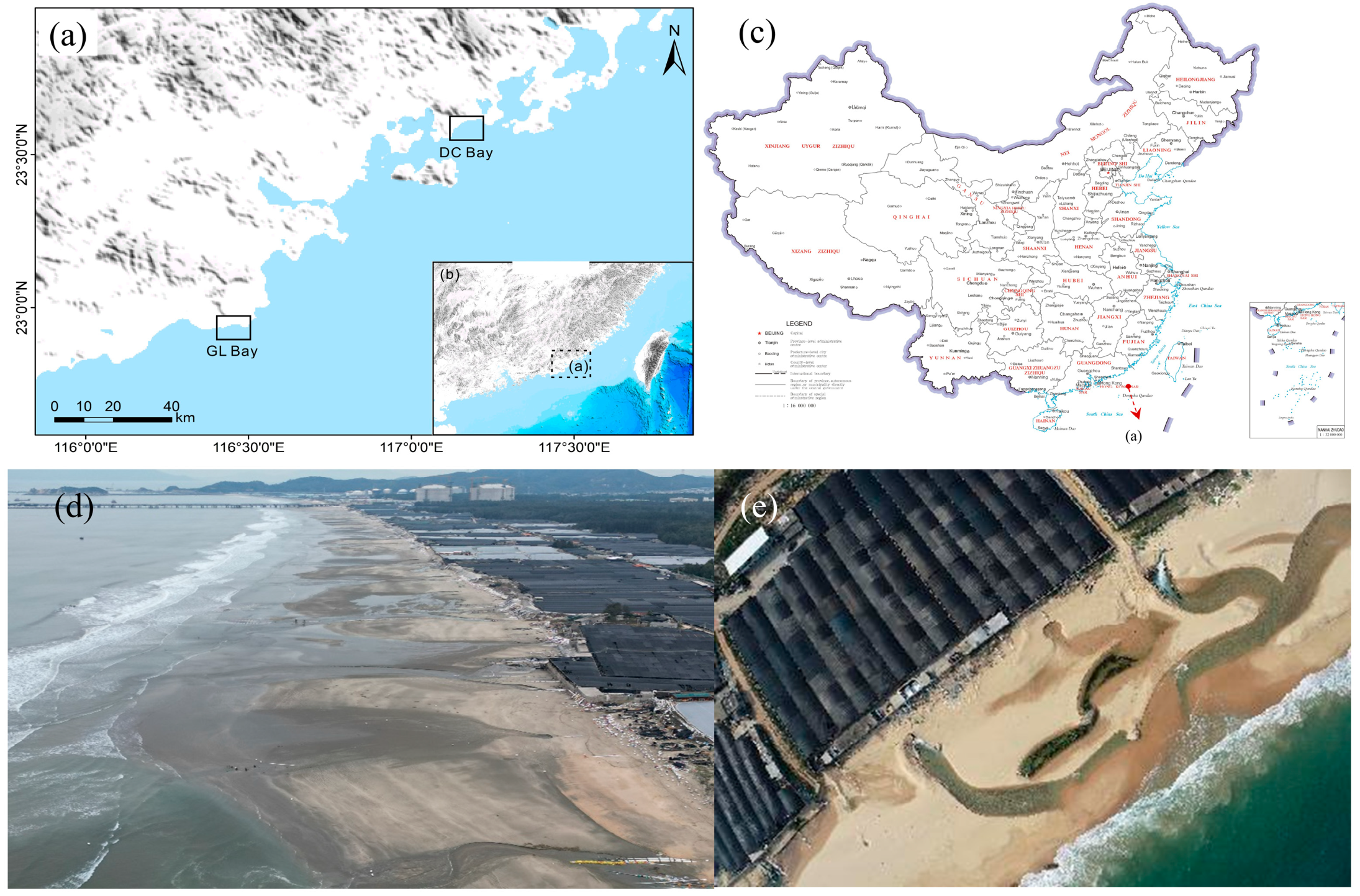
2.1. Description of the Field Site

The beach examined in the first case is located in Dacheng Bay (DC Bay in Figure 5a) between Fujian and Guangdong Provinces. The beach is a typical sandbar–lagoon beach with a sand spit that is primarily developed at the east end of the bay. The tides in the bay are semi-diurnal (irregular) and have a mean tidal range of 2.30 m. According to previous studies [38], littoral sedimentary processes in the bay were mainly driven by waves. Waves are dominated by wind waves, whose directions, wave energy, and frequency have obvious seasonality throughout the year. N-orientated winds and waves are prevalent in the bay during most months. According to the hindcast wave database of the Chinese Mainland [39], the wave conditions in Dacheng Bay are moderate, with an annual mean wave height of approximately 0.99 m (and a water depth of 20 m). The length of the coastline is approximately 15 km [38]. The coastline has a semilunar shape, and the mouth of the bay is oriented towards the SE. In this study, only a small part of the beach, which is backed by densely distributed coastal aquacultural ponds, is studied (hereafter, this area is referred to as Dacheng beach for convenience), as can be seen in Figure 5b. Dacheng beach mainly consists of fine-to-medium sediments with a mean grain diameter of approximately 0.25 mm, except for the headlands at the ends and a small section of bedrock coast in the middle part of the beach.

Gangliao bay (GL Bay in Figure 5a) is a key bay in the eastern Guangdong waters, which is a key area for the transition between the ecosystems of the East China Sea and those of the South China Sea, and is rich in natural resources such as islands, bays, and beaches. Gangliao bay is oriented towards the southeast, and the bay is generally rectangular in shape; the length of the coastline is approximately 12 km. The tides in Gangliao bay are diurnal (irregular) with a mean tidal range less than 1.5 m. According to a nearby wave buoy at Shenquan port, the annual maximum wave height is 4.77 m, while the average wave height was 0.43 m in 2020. The beach in Gangliao bay is a typical coastal compartment that consists of five continuous embayed units [40]. One of the relatively independent units (where the observation of sediment exchange between nearby units is very limited) will be used for shoreline modeling.

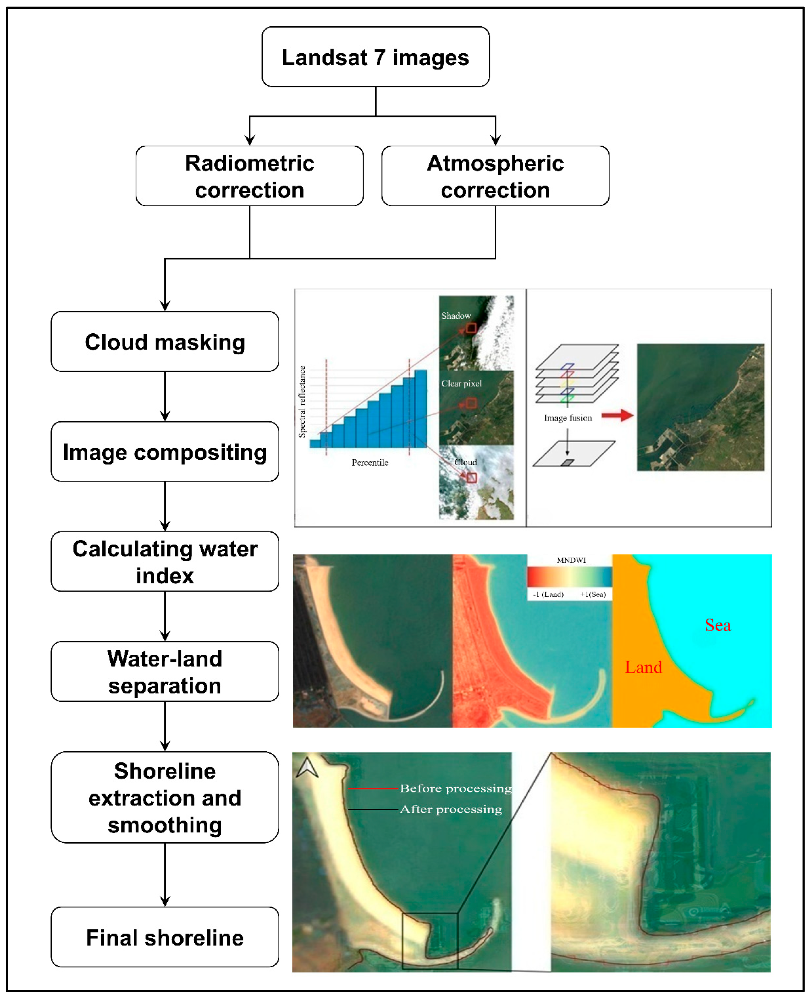
2.2. Remote Sensing of Shorelines from Satellites

In this study, approximately 870 Landsat 7 Surface Reflectance Tier 1 images were processed on the Google Earth Engine (GEE) platform [41]. The spatial resolution of the images was 30 m [42]. Raw satellite imagery is not suitable for direct shoreline detection due to atmospheric interference, cloud contamination, and sensor variability. Therefore, radiometric and atmospheric corrections were applied to produce surface reflectance imagery. Radiometric correction converts DN values to spectral radiance using sensor calibration coefficients as follows:

$$L_{\lambda }=M_L\times Q_{cal}+A_L$$

(1)

where $L_{\lambda }$ is the spectral radiance, $M_L$ is the radiance multiplicative factor, $Q_{cal}$ is the DN value, and $A_L$ is the radiance additive factor. Top-of-atmosphere reflectance (TOA) is then calculated as follows:

$${\rho }_p={\displaystyle \frac{\pi \times L_{\lambda }\times d^2}{{ESUN}_{\lambda }\times \cos {\theta }_S}}$$

(2)

where d is the Earth–Sun distance, ${ESUN}_{\lambda }$ is the mean solar exoatmospheric irradiance, and ${\theta }_S$ is the solar zenith angle. Atmospheric correction removes scattering and absorption effects to retrieve the true surface reflectance (SR). Based on the Dark Object Subtraction (DOS1) model, the corrected reflectance is as follows:

$$\rho ={\displaystyle \frac{\pi \times (L_{\lambda }-L_P)\times d^2}{T_v\times ({ESUN}_{\lambda }\times \cos {\theta }_S\times T_Z+E_{down})}}$$

(3)

where $L_P$ is the path radiance, $T_v$ and $T_Z$ are atmospheric transmittances, and $E_{down}$ is the downwelling diffuse irradiance. Under DOS1, $T_v$ = $T_Z$ = 1, and $E_{down}$ = 0.

Cloud masking was conducted using the CFMask algorithm integrated within GEE [43], which identifies cloud pixels based on multi-band decision trees and geometric projection. To address cloud-related data gaps, multi-temporal compositing was used to produce gap-filled surface reflectance images for each year [44,45].

After preprocessing, shoreline extraction was performed using a multi-step process including water index calculation, land–water classification, clustering, and boundary smoothing. Both the NDWI [46] and MNDWI [47] indices were computed as follows:

$$NDWI={\displaystyle \frac{{\rho }_{green}-{\rho }_{nir}}{{\rho }_{green}+{\rho }_{nir}}}\hspace{1em}MNDWI={\displaystyle \frac{{\rho }_{green}-{\rho }_{mir}}{{\rho }_{green}+{\rho }_{mir}}}$$

(4)

where ρ_green, ρ_nir, and ρ_mir are reflectance values of the green, near-infrared, and mid-infrared bands, respectively. Pixels with positive index values were classified as water, and negative values were classified as land.

The threshold for land–water segmentation was determined using the Otsu algorithm [48], which identifies the optimal value that maximizes between-class variance in the histogram of the index image.

Post-classification, morphological clustering was performed based on kernel functions tailored to local coastal geomorphology. To address the staircase appearance of extracted waterlines due to pixel shape, smoothing and sub-pixel refinement were applied. A forward algorithm of the Hidden Markov Model (HMM) was employed to generate continuous and regular shoreline contours [49].

To reduce the influence of tidal variation and short-term hydrodynamic effects (e.g., wave setup and storm surges), all available images within a calendar year were composited to extract an annual mean shoreline [50,51,52,53]. This shoreline represents the average waterline under mean sea level conditions and is suitable for long-term shoreline evolution analysis.

A detailed description of the shoreline data extraction can be found in the work of Chi et al. [22], who detected the shoreline evolution of paired sand spits from 1984 to 2020 on the Chinese Mainland. The flowchart of shoreline extraction from Landsat 7 imagery is provided in Figure 6.

2.3. High-Efficiency Shoreline Model

The ShorelineS model is based on one-line theory, and its governing equation is written as follows:

$${\displaystyle \frac{\partial n}{\partial t}}=-{\displaystyle \frac{1}{D_{\mathrm{c}}}}{\displaystyle \frac{\partial Q_{\mathrm{s}}}{\partial s}}-{\displaystyle \frac{\mathrm{RSLR}}{\tan \beta }}+{\displaystyle \frac{1}{D_{\mathrm{c}}}}\sum q_{\mathrm{i}}$$

(5)

where n represents the shoreline coordinate in the cross-shore direction; t is the time; D_c is the active profile height; Q_s is the longshore sediment transport rate; s is the alongshore coordinate; RSLR is the relative sea level rise; tanβ is the slope of the active profile; and q_i represents sources and sinks, including cross-shore sediment transport, sand nourishment, mining, etc. In the model setting, the active profile height Dc is chosen as 6 m. The most authoritative approach for determining the active profile height (D_c) is through a multi-year comparison of measured beach profiles to identify the depth beyond which no significant morphological change occurs. However, in practice, conducting repeated topographic and bathymetric surveys over long time periods is highly challenging. In our study, D_c = 6 m was selected based on a combination of regional wave climate characteristics and reference values, which were commonly adopted in previous studies of similar coastal settings. Specifically, this value corresponds approximately to the depth of closure d_c and the height from the upper berm limit to the mean sea level d_m under the local wave climate, where significant morphological change is expected to cease over seasonal to interannual time scales. Although no in situ measurement of closure depth is available for our site, the selected value is consistent with estimates from the literature using empirical formulas such as those from Hallermeier or Birkemeier [54,55], which relate D_c to significant wave height and wave period. For example, Hallermeier’s equation can be applied as follows:

$$d_c=2.28H_s-68.5{\displaystyle \frac{H_s^2}{g{T}^2}}$$

(6)

In this equation, typical storm wave conditions in our study area (e.g., H_s = 3.0 m and T = 6 s) can yield a closure depth in the order of 5.0 m. Given that the study focuses on decadal-scale shoreline dynamics and regional average conditions, we believe this choice of D_c is reasonable and consistent with established practices by assuming d_m is an order of half of the tidal range (approximately 1.0 m).

The longshore sediment transport rate is estimated using the CERC formula [56], as follows:

$$Q_{\mathrm{s}}=b{H}_{\mathrm{s}}^{5/2}\sin 2{\phi }_{\mathrm{loc}}$$

(7)

in which b represents the transport coefficient, H_s is the offshore significant wave height, and φ_loc is the incident wave angle. The governing equation is resolved using an improved vector-based grid. The transport coefficient b in the CERC formula is 2.3 × 10⁴ m^0.5/yr for the present case. Strictly speaking, the value of b should ideally be determined through site-specific calibration using long-term measured sediment transport rates, as it reflects the actual transport efficiency under local wave and sediment conditions. However, such field data are not available for our study site, and we acknowledge this as a limitation. In this study, our goal is not to simulate the detailed sediment transport process, but rather to use the CERC formula as part of an integrated framework to evaluate the relative spatial variation in shoreline response. As such, the transport coefficient b is treated as a tunable parameter that ensures that the model produces realistic spatial patterns of shoreline response, rather than a physically calibrated quantity.

3. Results

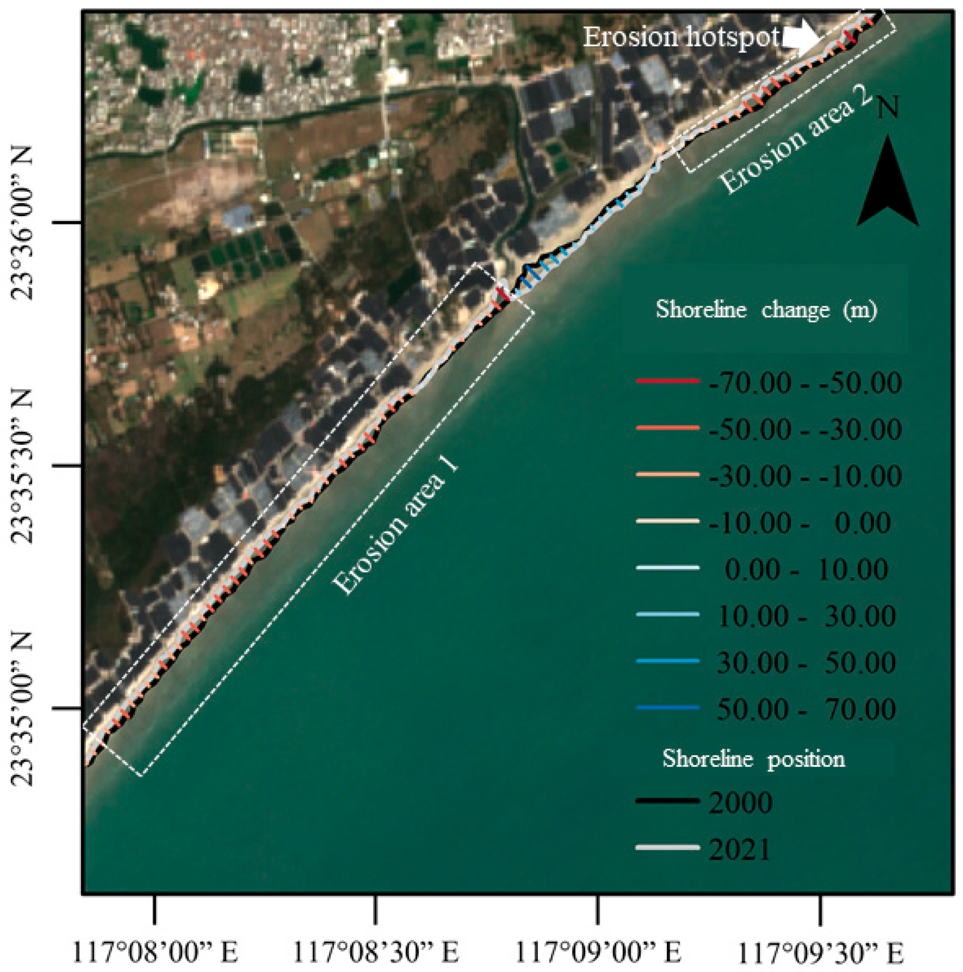
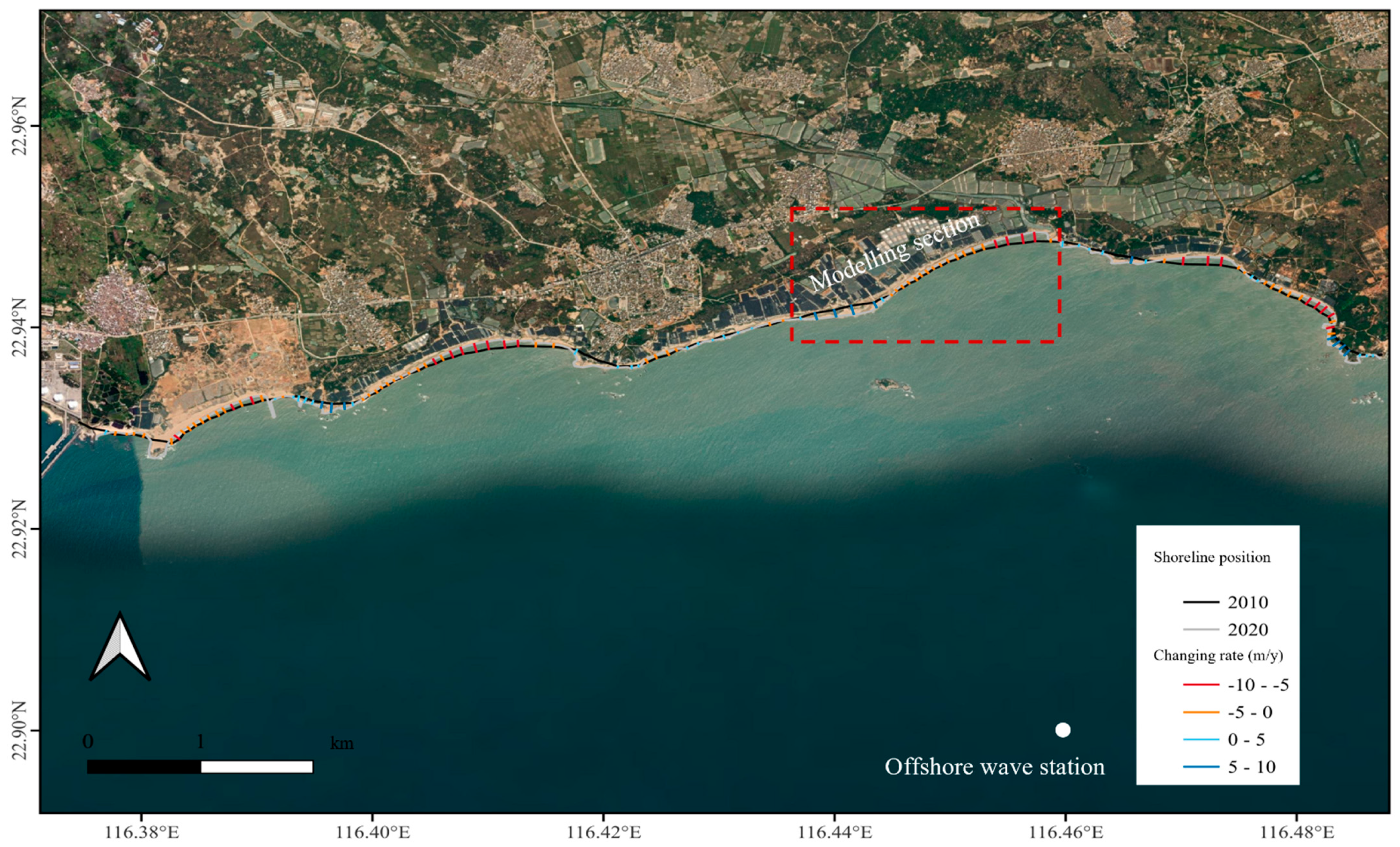
3.1. Satellite-Derived Shoreline Retreat

As can be seen in Figure 7, most of the shoreline experienced significant retreat in the period of 2000–2021 on Dacheng beach. The maximum shoreline retreat was up to 70 m in the past 20 years (the positive value means shoreline advance and vice versa). The erosion hotspot occurs on the northeast part of Dacheng beach, with a maximum annual rate of shoreline retreat of 3.5 m/y. In the middle part of Dacheng beach, a slight shoreline advance can be observed due to the sediment supply from a small estuary. By comparing shoreline positions in 2010 and 2021, the maximum shoreline retreats occur in the middle part of each embayed unit. The annual rate of shoreline retreats can be up to 10 m/y.

As can be seen in Figure 8, the magnitude of the shoreline retreat rate of Gangliaowan beach is generally larger than that of Dacheng beach. Although the annual mean wave height in Gangliao bay (0.94 m) is generally smaller than that in Dacheng Bay, embayed units are divided by rocks or breakwaters that limit the sediment supply in the longshore direction. There are six embayed units along the coastline of Gangliaowan beach, and severe beach erosion (or shoreline retreat) occurs in the middle of each embayed unit. The annual shoreline retreat can reach up to 5–10 m/y. The erosion of beaches backed by densely distributed coastal aquaculture ponds is more severe than those of natural beaches eroded by storms or rising sea levels. According to the China Sea Level Bulletin, part of the sandy shoreline of mainland China retreated by an average of 2.7 m due to sea level increases or storms in 2023. For tourist beaches, such as Qinghuangdao beach, the annual average rate of shoreline retreats only ranged from 0.5 m/y to 1.5 m/y [57].

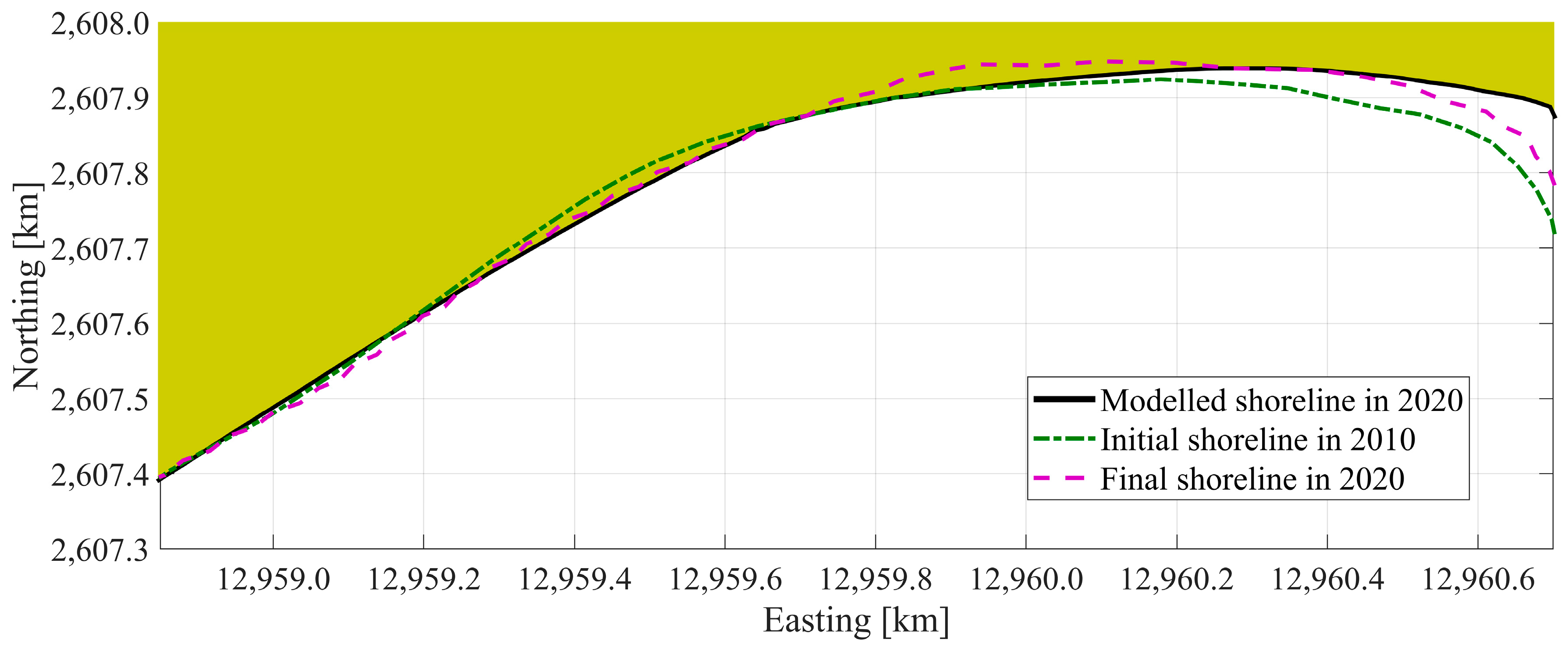
3.2. Verification of Shoreline Model

One of the embayed units is used to verify the shoreline evolution model, as shown in the red box in Figure 8. This is because on both sides of the unit, the shoreline is rather stable, indicating that the sediment exchange between nearby units is negligible. The offshore wave condition that drives the ShorelineS model was obtained from a hindcast regional wave model based on TOMAWAC [39] at a water depth of 15 m (22.90° N, 116.46° E), which is shown by the white point in Figure 8. The wave input includes significant wave heights, peak periods, and wave directions. The modeled time ranges from 1st January 2020 to 31st December 2020. The grid size is set as 12 m. The west and east boundaries are set as the fixed boundary condition (FIXD) and periodic boundary condition (PRDC), respectively.

Figure 9 provides a comparison between modeled and satellite-derived shorelines in 2020. It can be seen that the model correctly predicts the trend of shoreline evolution, i.e., shoreline retreat in the east part, shoreline advances in the middle section, and insignificant changes in the west part; however, the model overestimates the shoreline retreat in the west part. In addition, the shoreline advances are well modeled. To quantify the model performance, the Brier Skill Score (BSS) is used, which is defined as follows [58]:

$$\mathrm{BSS}=1 - {\displaystyle \frac{\sqrt{\frac{1}{L}{\int }_0^L{r}_{\mathrm{model}\left(\mathrm{s}\right) - \mathrm{measure}(\mathrm{s})}^2\mathrm{d}s}}{\sqrt{\frac{1}{L}{\int }_0^L{r}_{\mathrm{measure}\left(\mathrm{s}\right) - \mathrm{initial}\left(\mathrm{s}\right)}^2\mathrm{d}s}}}$$

(8)

where r represents the bias between the modeled and satellite-derived shoreline, s is the position of each shoreline segment, and L is the length of the shoreline. For the present case, the BSS is calculated as 0.55, indicating a moderate match between the modeled and satellite-derived shoreline. Therefore, this model is used to model future shoreline evolution in the next section.

4. Discussion

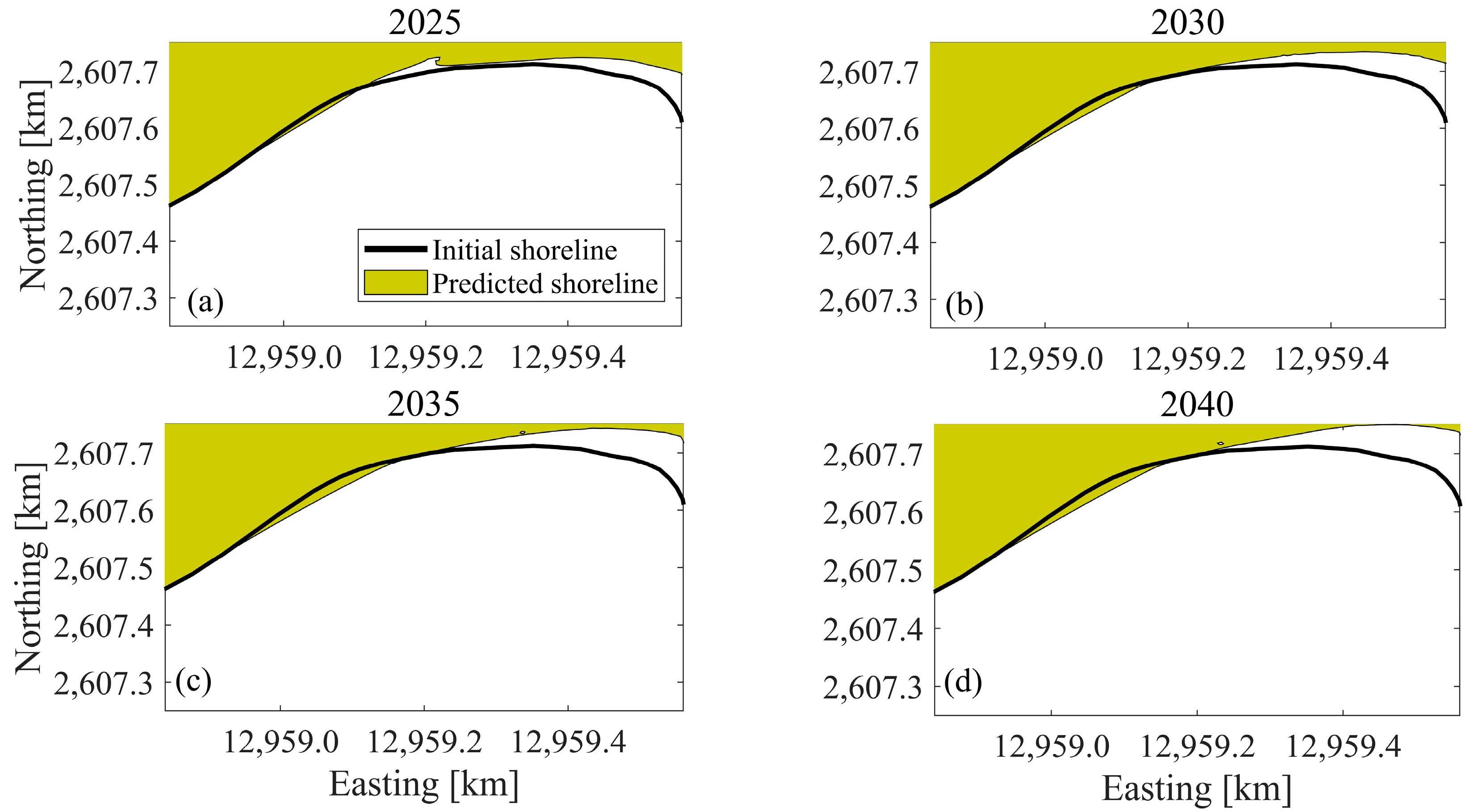
4.1. Future Shoreline Evolution

The verified ShorelineS model is used to predict the future evolution of shoreline that is backed by densely distributed coastal aquacultural ponds. Taking the satellite-derived shoreline in 2010 as the initial shoreline, the shoreline positions in 2025, 2030, 2035, and 2040 are modeled. The model parameters are kept the same as in the previous section. The offshore wave conditions that drive the model are expressed by wave climates, which consists of wave heights, peak periods, wave directions, and occurrence probability. The wave climate is generated by the hourly wave data from 2010 to 2020, which are extracted from the regional hindcast wave model of Shi et al. [39] (which is the same as in the previous section). As can be seen in Figure 10, the 10-year hourly wave data are separated into 50 bins according to the wave direction, and the total wave energy in each bin is equal. Then, the bulk wave parameters of each bin are statistically calculated to represent each wave condition.

It can be seen from Figure 11 that the east part of the embayment will experience continuous erosion in the future. The retreat distance of the erosion hotspot (defined as the position with the maximum distance of shoreline retreat) will increase from 150 m in 2025 to 240 m in 2040. At that time, the beach will lose all of its dry part. Shoreline advances can be observed in the middle part of the embayment. Compared with the shoreline retreat, shoreline advance is very limited. This only increases from 10 m in 2025 to 50 m in 2040. Furthermore, in 2025, the sand spit in the middle part of the embayment can be observed due to the high-inclination incident waves. However, the shoreline will achieve quasi-equilibrium after 2030. Due to the severe erosion of these beaches that are backed by coastal aquacultural ponds, strategies for beach protection are provided in the next section.

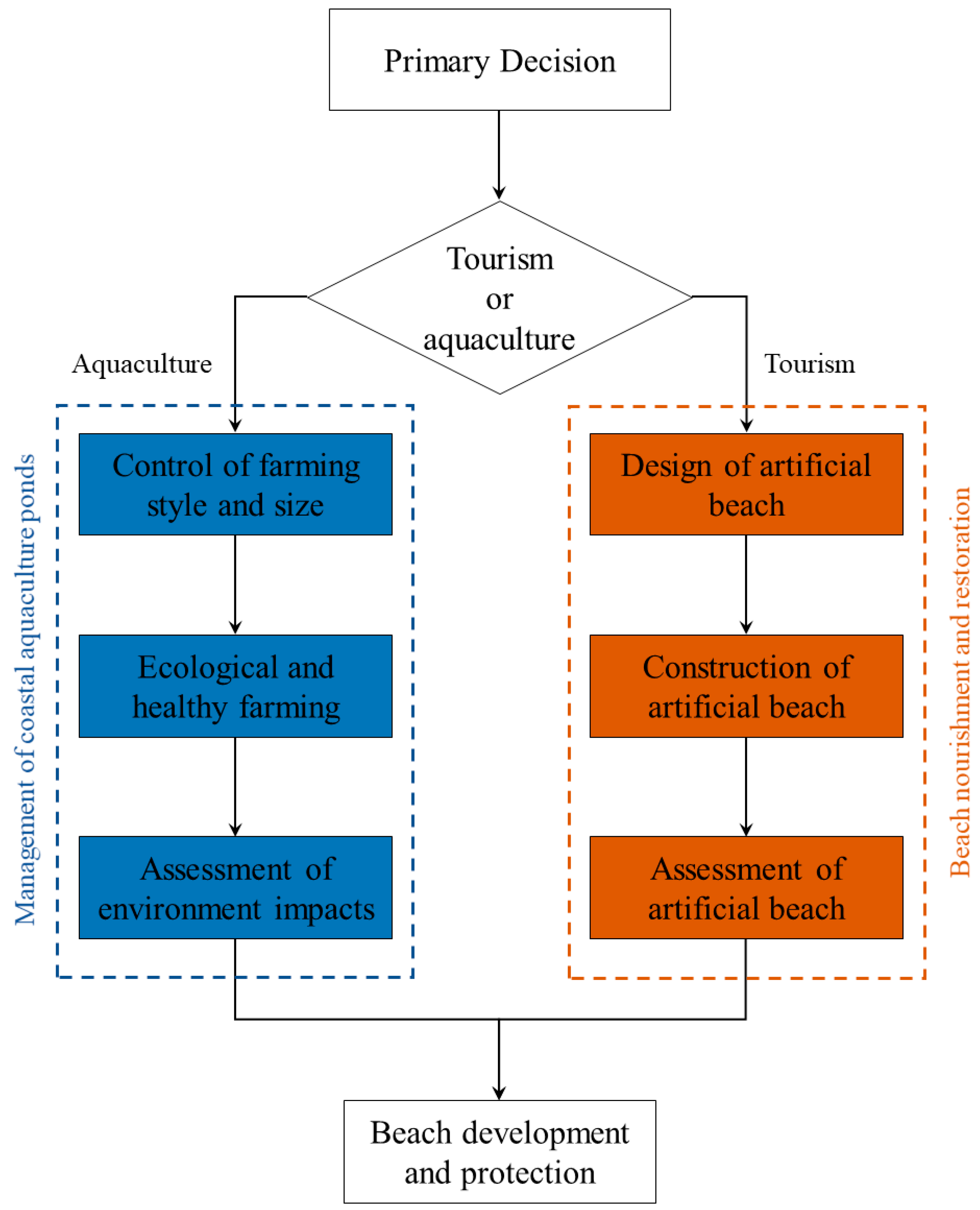
4.2. Strategies for Beach Protection

With the growing awareness of the negative environmental impacts of coastal aquaculture ponds, their remediation has been explored in recent years. The area of coastal aquaculture ponds in China decreased by 13.2% from 2016 to 2021 [15]. In addition, wind plays a crucial role in coastal dune formation and sediment transport, acting as a natural mechanism for beach nourishment and coastal protection. Aeolian processes help transport sand from the foreshore to the backshore, contributing to dune development, which serves as a natural buffer against wave action and storm surges. Additionally, wind-driven sediment transport can counteract erosion by replenishing areas experiencing sand loss. However, in this study, we observed that coastal aquaculture ponds contribute to beach erosion and surface “blackening”, which, in turn, reduces the effective fetch length and sand supply for wind-driven transport, thereby limiting dune formation. Moreover, the effectiveness of aeolian processes can be further influenced by vegetation cover, human interventions, and coastal morphology. Potential solutions to this hazard of beaches may include the management of coastal aquaculture ponds and beach nourishment, as can be seen in Figure 12. A primary decision on whether the sandy coast is used for aquaculture or tourism should be made before selecting a solution for beach development and protection. For example, if a sandy beach is used for tourism, coastal aquaculture ponds need to be relocated collectively to free up space for the construction of artificial beaches and the planting of protective forests. Similarly, if a beach is used for aquaculture, the environmentally friendly management of coastal aquaculture ponds and some simple remediation and restoration measures are required to ensure the relative stability of the beach. Specific practices or measures for the management of coastal aquaculture ponds, as well as beach nourishment and restoration, are provided below.

Management strategies include the control of farming style and size, ecological and healthy farming, and the post-assessment of environmental impacts. The prerequisite for the control of farming methods and scale is a clear knowledge of the local ecological carrying capacity. China’s Ministry of Ecology and Environment (MOE) and Ministry of Agriculture and Rural Affairs (MARD) issued a document in 2022 stipulating that farming areas are delineated according to a program of prohibited farming areas, restricted farming areas, and farming areas [59,60]. It also pointed out that the use of aquaculture waters and mudflats should be strictly regulated, and the spatial distribution of aquaculture should be further optimized to prohibit farming activities in areas that are prohibited by the law. The second is ecological and healthy farming, which encourages the development of advanced techniques or environmentally friendly materials that facilitate ecological and healthy farming modes. Existing coastal pond discharge systems should be remediated, while discharge pipes that are laid directly on the beach, which are installed illegally, should be strictly prohibited. For centrally distributed small- and medium-sized aquaculture outfalls, combined cleaning, the unified collection and treatment of aquaculture wastewater, and the setup of unified discharges should be encouraged. Key information such as the distribution of discharge outlets, their number, mode of discharge, time and frequency of discharge, and the direction of discharge should be checked and filed [59,60]. On this basis, wastewater discharge standards are formulated to specify discharge control indicators and limits for suspended solids, total nitrogen, total phosphorus, and chemical oxygen demand in the wastewater tailings. Finally, the environmental impact on beaches needs to be assessed, especially for new, renovated, and expanded coastal aquaculture construction projects. The management of coastal aquaculture ponds is guided by a document issued by the national department (i.e., the Ministry of Ecology and Environment, the Ministry of Agriculture and Rural Affairs, and the State Oceanic Administration), and specific policies are enacted and implemented by local departments. Examples of policy documents on the management of aquaculture at various levels of departments are listed in

Table 1. Policy documents on the management of aquaculture at different levels of departments.

Time	Department	Level	Name of the Policy Document
2022	Ministry of Ecology and Environment; Ministry of Agriculture and Rural Affairs	State	Opinions on strengthening the supervision and management of aquaculture ecosystems
2023	Ministry of Natural Resources; Ministry of Agriculture and Rural Affairs	State	Notice on the optimization of the management of sea use for aquaculture
2022	Department of Ecology and Environment of Guangdong Province; Department of Agriculture and Rural Development of Guangdong Province	Guangdong Province	Implementation program on strengthening the supervision and management of aquaculture ecosystems
2023	Department of Ecology and Environment of Fujian Province; Bureau of Ocean and Fisheries, Fujian Province	Fujian Province	Work program for tailwater management of marine aquaculture ponds in Fujian Province
2022	Bureau of Ecology and Environment of Chaozhou City	Chaozhou City	List of key tasks of the implementation program for strengthening the supervision and management of aquaculture ecosystems in Chaozhou City

.

Before commencing the beach restoration and nourishment project, general information on the restoration area should be obtained. This information includes geographic location, ecosystem status, the current state of utilization of marine areas, socio-economic information, and policy and implementation of previous projects. Second, the feasibility and necessity of the project should be analyzed according to the policy of the government and the practical needs for local ecosystem restoration. Then, the identification and diagnosis of ecosystem issues can be carried out. These issues mainly include the pollution from the direct discharge of farming wastewater, coastal pollution due to the indiscriminate disposal of household and production waste, and beach erosion caused by the pipes directly set on the beach surface.

The effective implementation of programs for mitigating pollution and beach erosion should be developed. These programs include the removal of waste and abandoned pipes from the surface of the beach, the excavation or burial of polluted sediment on the beach surface, the restoration of protected forests, and beach nourishment. The design of beach nourishment should consider the local hydrodynamic conditions, and the nearshore wave and water level data of the target area should be fully obtained from, e.g., globe or national hindcast wave data [39]. Topography measurements could be conducted using, e.g., the Real-Time Kinematic (RTK) method with a frequency of three times per month before the beach nourishment projects [61]. From the perspective of improving efficiency and saving costs, the profile after sand filling should be an equilibrium profile that is compatible with local dynamic conditions to minimize sediment loss after beach nourishment [62,63,64,65]. Process-based or empirical models of beach evolution can be used in the comparison of programs, as well as in the assessments of beach adaptability and stability [66,67].

After the completion of beach nourishment, the effect of nourishment will be continuously monitored, including topographic monitoring, ocean dynamics monitoring, and ecology monitoring. Topographic monitoring includes the location of the shoreline, the width of the dry beach, and the nearshore water depth; ocean dynamics monitoring includes wave height, water level, and wave direction; and ecology monitoring mainly includes water quality and sediments.

As mentioned above, potential solutions to beach hazards caused by coastal aquaculture ponds are generally introduced in terms of the management of coastal aquaculture ponds and beach nourishment. However, limited by the knowledge of the authors, completed projects of beach nourishment that are conducted on beaches backed by coastal aquaculture ponds are rather limited. This is because the function and positioning of the beaches are different from one region to another. In economically developed regions, such as Xiamen, beaches are nourished for tourism. These regions emphasize and are willing to manage and regularly restore and nourish their beaches. Furthermore, these regions have advanced neighborhood amenities such as convenient transportation (airports and high-speed railway networks), bustling shopping malls, and abundant hotels and restaurants. In the long run, positive feedback is created between the investments in beach nourishment and the income from beach tourism. For example, from 2012 to 2018, the total revenue income from direct beach tourism and its added value (CNY 112.575 billion plus CNY 45.007 billion) is far higher than the investment in beach nourishment programs [68]. The development of beach tourism will also lead to an increase in local house prices [69]. In contrast, in areas of relative poverty, there has been a relative lack of investment in beach tourism by local governments. Due to the poor surrounding facilities, underdeveloped transportation, and dirty beach environment, it is difficult to initiate the development of tourism. Therefore, the local government prefers to develop the coastal aquaculture economy to provide more employment opportunities. As the coastal zone protection and restoration projects in the Chinese mainland continue to advance, these regions are also faced with the problem of industrial and economic transformation. In the Chinese Mainland, funding for beach maintenance usually comes from local and central government finances. Typical beach nourishment projects have always been conducted in well-developed cities, such as Hong Kong, Xiamen, Qingdao, and Haikou [70], which is attributed to the abundance of local government finances. One of the implications is that central financial funds should be appropriately inclined towards coastal zone protection and restoration projects in remote areas far from developed cities to support the development of local beach tourism.

Thus far, completed projects of beach nourishment that are conducted on beaches backed by coastal aquaculture ponds are rather limited. This depends on the local economic situation, transportation conditions, and the degree of sophistication of tourism support facilities. The urbanization disparities in the protection and restoration of coastal zones need to be considered, as there is often a lack of funding and technology devoted to restoring beaches that are far away from developed cities. There should be a call for the central financial funds of the Chinese Mainland, which should be appropriately inclined towards coastal zone protection and restoration projects in remote areas far from developed cities, in order to support the development of local beach tourism and industry transformation.

4.3. Limitations of This Study

In this study, we define the shoreline as the land–water boundary corresponding approximately to the mean sea level (MSL). To reduce the influence of short-term hydrodynamic variability such as tides, wave run-up, or storm surges, we extract the annual mean shoreline for each year by compositing multiple cloud-free Landsat scenes. This approach effectively smooths out high-frequency fluctuations and yields a stable representation of shoreline position under average hydrological conditions. The annual mean shoreline thus corresponds to the same physical boundary across all years.

All shoreline positions were derived from Landsat surface reflectance products using a standardized workflow, including cloud masking (Fmask), MNDWI calculation, threshold segmentation, and morphological filtering. We applied the same classification criteria and parameters across the full timespan (2001–2021) to ensure comparability.

We acknowledge that independent ground-truth data (e.g., GPS surveys or UAV imagery) are not available for the study area, which is a limitation. However, our method follows established procedures that are widely used in long-term shoreline monitoring studies, which report horizontal uncertainties generally within 1–2 pixels (30–60 m) for Landsat-based shorelines.

Although the shoreline evolution model employed in this study includes a term associated with relative sea level rise (RSLR), we did not explicitly consider changes in wave conditions or closure depth over time. In the current implementation, the RSLR term remains part of the model formulation; however, this term is constant and decoupled from evolving hydrodynamic forcing. This simplification may underestimate or misrepresent the feedback between sea level rises and coastal morphodynamics, particularly in regions where rising water levels are accompanied by significant changes in wave climate or storm regimes [71,72,73].

It is important to acknowledge that the spatial resolution of Landsat imagery (30 m) introduces a horizontal uncertainty of approximately ±30 to ±60 m in the extracted shoreline positions. This inherent uncertainty can influence both the estimated shoreline retreat rates and the reliability of model-based future projections. In particular, when the magnitude of observed shoreline change is relatively small or the temporal coverage is short, the positional error may account for a substantial portion of the estimated change, thereby increasing the relative uncertainty of the results. In contrast, for beaches exhibiting more pronounced retreat trends over longer time periods, the effect of such uncertainty becomes comparatively less significant.

Moreover, this uncertainty may propagate through the model calibration process and affect future retreat predictions, especially in low-energy environments or sites with relatively stable shorelines. While our method captures the overall trend of shoreline change effectively, we recommend interpreting site-level results with caution where shoreline shifts are within or near the error margin. Higher-resolution imagery (e.g., Sentinel-2 or commercial satellite data) and in situ shoreline validation would help further improve accuracy and confidence in both historical analyses and forward-looking assessments.

Future research should aim to integrate sea level projections with dynamic wave conditions and shoreline response, for example, by coupling the one-line model with offshore wave models or empirical relationships that adjust closure depth and wave-driven transport rates in tandem. Such extensions would enable a more physically consistent assessment of shoreline migration under climate change scenarios.

5. Conclusions

In this study, satellite-derived shorelines of beaches backed by coastal aquaculture are provided. A high-efficiency model of shoreline evolution is verified by the satellite-derived shorelines, which is then used to predict the shoreline evolution in future years. Finally, strategies for beach protection are suggested. The main conclusions are drawn below.

A quantitative analysis of shoreline retreats on beaches backed by densely distributed coastal aquaculture ponds is conducted based on the Google Earth Engine. The erosion hotspot occurs on the northeast part of Dacheng beach, with a maximum annual rate of shoreline retreat of 3.5 m/y. On Gangliaowan beach, the maximum shoreline retreats occur in the middle part of each embayed unit, and the annual rate of shoreline retreats can be up to 10 m/y.

A high-efficiency shoreline evolution model is verified using the satellite-derived shoreline dataset. The model correctly predicts the trend of shoreline evolution. For the present case, the BSS is calculated as 0.55, indicating a moderate match between the modeled and satellite-derived shoreline. The verified ShorelineS model is then used to predict the future evolution of shoreline that is backed by densely distributed coastal aquacultural ponds. The retreat distance of the erosion hotspot (defined as the position with the maximum distance of shoreline retreat) will increase from 150 m in 2025 to 240 m in 2040. It is expected that the beach will lose all of its dry part in the future.

Potential strategies to protect the beach include the management of coastal aquaculture ponds and beach nourishment. The management of coastal aquaculture ponds refers to the planning of farming areas, the development of ecological farming techniques, the treatment of farming wastewater, and the post-assessment of the beach environment. Beach restoration and nourishment should include the removal of waste and abandoned pipes from the surface of the beach, the excavation or burial of polluted sediment on the beach surface, the restoration of protected forests, and beach nourishment.

References

1. Barbier, E.B.; Hacker, S.D.; Kennedy, C.; Koch, E.W.; Stier, A.C.; Silliman, B.R. The value of estuarine and coastal ecosystem services. Ecol. Monogr. 2011, 81, 169–193. [Google Scholar] [CrossRef]
2. Ranasinghe, R. Assessing climate change impacts on open sandy coasts: A review. Earth-Sci. Rev. 2016, 160, 320–332. [Google Scholar] [CrossRef]
3. Shi, J.; Feng, X.; Toumi, R.; Zhang, C.; Hodges, K.I.; Tao, A.; Zhang, W.; Zheng, J. Global increase in tropical cyclone ocean surface waves. Nat. Commun. 2024, 15, 174. [Google Scholar] [CrossRef]
4. Vousdoukas, M.I.; Ranasinghe, R.; Mentaschi, L.; Plomaritis, T.A.; Athanasiou, P.; Luijendijk, A.; Feyen, L. Sandy coastlines under threat of erosion. Nat. Clim. Chang. 2020, 10, 260–263. [Google Scholar] [CrossRef]
5. Third Institute of Oceanography, State Oceanic Administration. Coastal Erosion Assessment and Control: The Final Report, Chinese Offshore Investigation and Assessment; Third Institute of Oceanography, State Oceanic Administration: Xiamen, China, 2010; pp. 39–50. [Google Scholar]
6. Wang, X.; Yan, F.; Su, F. Changes in coastline and coastal reclamation in the three most developed areas of China, 1980–2018. Ocean. Coast. Manag. 2021, 204, 105542. [Google Scholar] [CrossRef]
7. Xu, N.; Gong, P. Significant coastline changes in China during 1991–2015 tracked by Landsat data. Sci. Bull. 2018, 63, 883–886. [Google Scholar] [CrossRef]
8. Xu, N.; Wang, Y.; Huang, C.; Jiang, S.; Jia, M.; Ma, Y. Monitoring coastal reclamation changes across Jiangsu Province during 1984–2019 using landsat data. Mar. Policy 2022, 136, 104887. [Google Scholar] [CrossRef]
9. Cai, F.; Cao, C.; Qi, H.; Su, X.; Lei, G.; Liu, J.; Zhao, S.; Liu, G.; Zhu, K. Rapid migration of mainland China’s coastal erosion vulnerability due to anthropogenic changes. J. Environ. Manag. 2022, 319, 115632. [Google Scholar] [CrossRef]
10. Ji, C.; Zhang, Q.; Chen, T.; Ma, D.; Huang, R. Modeling investigation of wave-induced longshore current distribution patterns on barred beaches. Estuar. Coast. Shelf Sci. 2024, 299, 108685. [Google Scholar] [CrossRef]
11. Li, Y.; Zhang, C.; Zhao, S.; Qi, H.; Cai, F.; Zheng, J. Equilibrium configurations of sandy-muddy transitional beaches on South China coasts: Role of waves in formation of sand-mud transition boundary. Coast. Eng. 2024, 187, 104401. [Google Scholar] [CrossRef]
12. Li, Y.; Zhang, C.; Chen, S.; Qi, H.; Dai, W.; Zhu, H.; Sui, T.; Zheng, J. Experimental Investigation on Cross-Shore Profile Evolution of Reef-Fronted Beach. Coast. Eng. 2025, 104653. [Google Scholar] [CrossRef]
13. Jiang, S.; Xu, N.; Li, Z.; Huang, C. Satellite derived coastal reclamation expansion in China since the 21st century. Glob. Ecol. Conserv. 2021, 30, e01797. [Google Scholar] [CrossRef]
14. Ministry of Agriculture and Rural Affairs, China National Aquatic Technology and Promotion Center, Chinese Society of Aquatic Sciences. China Fisheries Statistics Yearbook; China Agricultural Publishing House: Beijing, China, 2023. [Google Scholar]
15. Wang, M.; Mao, D.; Xiao, X.; Song, K.; Jia, M.; Ren, C.; Wang, Z. Interannual changes of coastal aquaculture ponds in China at 10-m spatial resolution during 2016–2021. Remote Sens. Environ. 2023, 284, 113347. [Google Scholar] [CrossRef]
16. Wang, Z.; Zhang, J.; Yang, X.; Huang, C.; Su, F.; Liu, X.; Liu, Y.; Zhang, Y. Global Mapping of the Landside Clustering of Aquaculture Ponds from Dense Time-Series 10 m Sentinel-2 Images on Google Earth Engine. Int. J. Appl. Earth Obs. Geoinf. 2022, 115, 103100. [Google Scholar] [CrossRef]
17. Gao, X.; Zhang, M.; Luo, X.; You, W.; Ke, C. Transitions, challenges and trends in China’s abalone culture industry. Rev. Aquac. 2023, 15, 1274–1293. [Google Scholar] [CrossRef]
18. Davidson, E.A.; Janssens, I.A. Temperature sensitivity of soil carbon decomposition and feedbacks to climate change. Nature 2006, 440, 165–173. [Google Scholar] [CrossRef]
19. Tan, L.; Zhang, L.; Yang, P.; Tong, C.; Lai, D.Y.F.; Yang, H.; Hong, Y.; Tian, Y.; Tang, C.; Ruan, M.; et al. Effects of conversion of coastal marshes to aquaculture ponds on sediment anaerobic CO2 production and emission in a subtropical estuary of China. J. Environ. Manag. 2023, 338, 117813. [Google Scholar] [CrossRef]
20. Lansu, E.M.; Reijers, V.C.; Höfer, S.; Luijendijk, A.; Rietkerk, M.; Wassen, M.J.; Lammerts, E.J.; van der Heide, T. A global analysis of how human infrastructure squeezes sandy coasts. Nat. Commun. 2024, 15, 432. [Google Scholar] [CrossRef]
21. Liu, S.; Wu, K.; Yao, L.; Li, Y.; Chen, R.; Zhang, L.; Wu, Z.; Zhou, Q. Characteristics and correlation analysis of heavy metal distribution in China’s freshwater aquaculture pond sediments. Sci. Total Environ. 2024, 931, 172909. [Google Scholar] [CrossRef]
22. Chi, S.; Zhang, C.; Wang, P.; Shi, J.; Li, F.; Li, Y.; Wang, P.; Zheng, J.; Sun, J.; Nguyen, V.T. Morphological evolution of paired sand spits at the Fudu river mouth: Wave effects and anthropogenic factors. Mar. Geol. 2023, 456, 106991. [Google Scholar] [CrossRef]
23. Liu, G.; Qi, H.; Cai, F.; Zhu, J.; Zhao, S.; Liu, J.; Lei, G.; Cao, C.; He, Y.; Xiao, Z. Initial morphological responses of coastal beaches to a mega offshore artificial island. Earth Surf. Process. Landf. 2022, 47, 1355–1370. [Google Scholar] [CrossRef]
24. Chi, S.-H.; Zhang, C.; Sui, T.-T.; Cao, Z.-B.; Zheng, J.-H.; Fan, J.-S. Field observation of wave overtopping at sea dike using shore-based video images. J. Hydrodyn. 2021, 33, 657–672. [Google Scholar] [CrossRef]
25. Bishop-Taylor, R.; Nanson, R.; Sagar, S.; Lymburner, L. Mapping Australia’s dynamic coastline at mean sea level using three decades of Landsat imagery. Remote Sens. Environ. 2021, 267, 112734. [Google Scholar] [CrossRef]
26. Turner, I.L.; Harley, M.D.; Almar, R.; Bergsma, E.W. Satellite optical imagery in coastal engineering. Coast. Eng. 2021, 167, 103919. [Google Scholar] [CrossRef]
27. Hanson, H. GENESIS: A generalized shoreline change numerical model. J. Coast. Res. 1989, 5, 1–27. [Google Scholar]
28. Kristensen, S.; Drønen, N.; Deigaard, R.; Fredsoe, J. Impact of groyne fields on the littoral drift: A hybrid morphological modelling study. Coast. Eng. 2016, 111, 13–22. [Google Scholar] [CrossRef]
29. Tonnon, P.K.; Huisman, B.J.A.; Stam, G.N.; van Rijn, L.C. Numerical modelling of erosion rates, life span and maintenance volumes of mega nourishments. Coast. Eng. 2018, 131, 51–69. [Google Scholar] [CrossRef]
30. Vitousek, S.; Barnard, P.L.; Limber, P.; Erikson, L.; Cole, B. A model integrating longshore and cross-shore processes for predicting long-term shoreline response to climate change. J. Geophys. Res. Earth Surf. 2017, 122, 782–806. [Google Scholar] [CrossRef]
31. Yates, M.L.; Guza, R.T.; O’reilly, W.C. Equilibrium shoreline response: Observations and modeling. J. Geophys. Res. 2009, 114, C09014. [Google Scholar] [CrossRef]
32. Bruun, P. Sea-level rise as cause of shore erosion. J. Waterw. Harb. Div. 1962, 88, 117–130. [Google Scholar] [CrossRef]
33. Robinet, A.; Idier, D.; Castelle, B.; Marieu, V. A reduced-complexity shoreline change model combining longshore and cross-shore processes: The LX-shore model. Environ. Model. Softw. 2018, 109, 1–16. [Google Scholar] [CrossRef]
34. Davidson, M.A.; Splinter, K.D.; Turner, I.L. A simple equilibrium model for predicting shoreline change. Coast. Eng. 2013, 73, 191–202. [Google Scholar] [CrossRef]
35. Kaergaard, K.; Fredsoe, J. A numerical shoreline model for shorelines with large curvature. Coast. Eng. 2013, 74, 19–32. [Google Scholar] [CrossRef]
36. Hurst, M.D.; Barkwith, A.; Ellis, M.A.; Thomas, C.W.; Murray, A.B. Exploring the sensitivities of crenulate bay shorelines to wave climates using a new vector-based one-line model. J. Geophys. Res. Earth Surf. 2015, 120, 2586–2608. [Google Scholar] [CrossRef]
37. Roelvink, D.; Huisman, B.; Elghandour, A.; Ghonim, M.; Reyns, J. Efficient modeling of complex sandy coastal evolution at monthly to century time scales. Front. Mar. Sci. 2020, 7, 535. [Google Scholar] [CrossRef]
38. Cai, F.; Su, X.; Gao, Z.; Chen, J. Stability analysis and beach protection countermeasures of Dacheng Bay at the junction of Fujian and Guangdong. Taiwan Strait 2003, 4, 518–525. [Google Scholar]
39. Shi, J.; Zheng, J.; Zhang, C.; Joly, A.; Zhang, W.; Xu, P.; Sui, T.; Chen, T. A 39-year high resolution wave hindcast for the Chinese coast: Model validation and wave climate analysis. Ocean. Eng. 2019, 183, 224–235. [Google Scholar] [CrossRef]
40. Carvalho, R.C.; Woodroffe, C.D. Coastal compartments: The role of sediment supply and morphodynamics in a beach management context. J. Coast. Conserv. 2023, 27, 58. [Google Scholar] [CrossRef]
41. Gorelick, N.; Hancher, M.; Dixon, M.; Ilyushchenko, S.; Thau, D.; Moore, R. Google Earth Engine: Planetary-scale geospatial analysis for everyone. Remote Sens. Environ. 2017, 202, 18–27. [Google Scholar] [CrossRef]
42. Vermote, E.; Justice, C.; Claverie, M.; Franch, B. Preliminary analysis of the performance of the Landsat 8/OLI land surface reflectance product. Remote Sens. Environ. 2016, 185, 46–56. [Google Scholar] [CrossRef]
43. Zhu, Z.; Woodcock, C.E. Object-based cloud and cloud shadow detection in Landsat imagery. Remote Sens. Environ. 2012, 118, 83–94. [Google Scholar] [CrossRef]
44. U.S. Geological Survey. Landsat 8 (L8) Data Users Handbook. 2019. Available online: https://www.usgs.gov/landsat-missions/landsat-8-data-users-handbook (accessed on 1 June 2024).
45. Foga, S.; Scaramuzza, P.L.; Guo, S.; Zhu, Z.; Dilley, R.D.; Beckmann, T.; Schmidt, G.L.; Dwyer, J.L.; Hughes, M.J.; Laue, B. Cloud detection algorithm comparison and validation for operational Landsat data products. Remote Sens. Environ. 2017, 194, 379–390. [Google Scholar] [CrossRef]
46. McFeeters, S.K. The use of the Normalized Difference Water Index (NDWI) in the delineation of open water features. Int. J. Remote Sens. 1996, 17, 1425–1432. [Google Scholar] [CrossRef]
47. Xu, H. Modification of normalised difference water index (NDWI) to enhance open water features in remotely sensed imagery. Int. J. Remote Sens. 2006, 27, 3025–3033. [Google Scholar] [CrossRef]
48. Otsu, N. A threshold selection method from gray-level histograms. IEEE Trans. Syst. Man Cybern. 1979, 9, 62–66. [Google Scholar] [CrossRef]
49. Rabiner, L.R. A tutorial on hidden Markov models and selected applications in speech recognition. Proc. IEEE 1989, 77, 257–286. [Google Scholar] [CrossRef]
50. Almonacid-Caballer, J.; Sánchez-García, E.; Pardo-Pascual, J.E.; Balaguer-Beser, A.A.; Palomar-Vázquez, J. Evaluation of annual mean shoreline position deduced from Landsat imagery as a mid-term coastal evolution indicator. Mar. Geol. 2016, 372, 79–88. [Google Scholar] [CrossRef]
51. Xu, N. Detecting coastline change with all available landsat data over 1986–2015: A case study for of Texas, USA. Atmosphere 2018, 9, 107. [Google Scholar] [CrossRef]
52. Cao, W.; Zhou, Y.; Li, R.; Li, X. Mapping changes in coastlines and tidal flats in developing islands using the full time series of Landsat images. Remote Sens. Environ. 2020, 239, 111665. [Google Scholar] [CrossRef]
53. Ding, Y.; Yang, X.; Jin, H.; Wang, Z.; Liu, Y.; Liu, B.; Zhang, J.; Liu, X.; Gao, K.; Meng, D. Monitoring coastline changes of the Malay Islands based on Google Earth Engine and dense time-series remote sensing images. Remote Sens. 2021, 13, 3842. [Google Scholar] [CrossRef]
54. Hallermeier, R.J. Uses for a calculated limit depth to beach erosion. Coast. Eng. Proc. 1978, 1, 88. [Google Scholar] [CrossRef]
55. Birkemeier, W.A. Field data on seaward limit of profile change. J. Waterw. Port Coast. Ocean. Eng. 1985, 111, 598–602. [Google Scholar] [CrossRef]
56. USACE. Shore Protection Manual; US Army Corps of Engineers: Washington, DC, USA, 1984. [Google Scholar]
57. Ministry of Natural Resources. 2023 China Sea Level Bulletin; Ministry of Natural: Beijing, China, 2024. (In Chinese)
58. Sutherland, J.; Peet, A.H.; Soulsby, R.L. Evaluating the performance of morphological models. Coast. Eng. 2004, 51, 917–939. [Google Scholar] [CrossRef]
59. Ministry of Ecology and Environment. Opinions on Strengthening the Supervision and Management of Aquaculture Ecosystems. 2022. Available online: https://www.gov.cn/zhengce/zhengceku/2022-01/12/content_5667762.htm (accessed on 1 June 2024).
60. Ministry of Natural Resources and Ministry of Agriculture and Rural Affairs. Notice on Optimization of Management of Sea Use for Aquaculture. 2023. Available online: https://www.gov.cn/zhengce/zhengceku/202312/content_6923452.htm (accessed on 1 June 2024).
61. China Association of Oceanic Engineering. Technical Guideline on Coastal Ecological Rehabilitation for Hazard Mitigation; China Association of Oceanic Engineering: Nanjing, China, 2020. [Google Scholar]
62. Li, Y.; Zhang, C.; Chen, D.; Zheng, J.; Sun, J.; Wang, P. Barred beach profile equilibrium investigated with a process-based numerical model. Cont. Shelf Res. 2021, 222, 104432. [Google Scholar] [CrossRef]
63. Li, Y.; Zhang, C.; Dai, W.; Chen, D.; Sui, T.; Xie, M.; Chen, S. Laboratory investigation on morphology response of submerged artificial sandbar and its impact on beach evolution under storm wave condition. Mar. Geol. 2022, 443, 106668. [Google Scholar] [CrossRef]
64. Liu, G.; Cai, F.; Qi, H.; Zhu, J.; Liu, J. Morphodynamic evolution and adaptability of nourished beaches. J. Coast. Res. 2019, 35, 737–750. [Google Scholar] [CrossRef]
65. Liu, G.; Cai, F.; Qi, H.; Zhu, J.; Lei, G.; Cao, H.; Zheng, J. A method to nourished beach stability assessment: The case of China. Ocean. Coast. Manag. 2019, 177, 166–178. [Google Scholar] [CrossRef]
66. Ruessink, B.G.; Kuriyama, Y.; Reniers, A.J.H.M.; Roelvink, J.A.; Walstra, D.J.R. Modeling cross-shore sandbar behavior on the timescale of weeks. J. Geophys. Res. Earth Surf. 2007, 112, 03010. [Google Scholar] [CrossRef]
67. Zheng, J.; Zhang, C.; Demirbilek, Z.; Lin, L. Numerical study of sandbar migration under wave-undertow interaction. J. Waterw. Port Coast. Ocean. Eng. 2014, 140, 146–159. [Google Scholar] [CrossRef]
68. Yang, W.; Cai, F.; Liu, J.; Zhu, J.; Qi, H.; Liu, Z. Beach economy of a coastal tourist city in China: A case study of Xiamen. Ocean. Coast. Manag. 2021, 211, 105798. [Google Scholar] [CrossRef]
69. Armstrong, S.B.; Lazarus, E.D.; Limber, P.W.; Goldstein, E.B.; Thorpe, C.; Ballinger, R.C. Indications of a positive feedback between coastal development and beach nourishment. Earth’s Future 2016, 4, 626–635. [Google Scholar] [CrossRef]
70. Liu, G.; Cai, F.; Qi, H.; Liu, J.; Lei, G.; Zhu, J.; Cao, H.; Zheng, J.; Zhao, S.; Yu, F. A summary of beach nourishment in China: The past decade of practices. Shore Beach 2020, 2020, 65–73. [Google Scholar] [CrossRef]
71. Ranasinghe, R.; Stive, M.J.F.; Roelvink, D. Modelling of climate-change-induced shoreline change. Clim. Chang. 2012, 110, 561–576. [Google Scholar] [CrossRef]
72. Le Cozannet, G.; Bulteau, T.; Castelle, B.; Ranasinghe, R.; Wöppelmann, G.; Rohmer, J.; Bernon, N.; Idier, D.; Louisor, J.; Salas-Y-Mélia, D. Quantifying uncertainties of sandy shoreline change projections as sea level rises. Sci. Rep. 2019, 9, 42. [Google Scholar] [CrossRef]
73. Hinkel, J.; Lincke, D.; Vafeidis, A.T.; Perrette, M.; Nicholls, R.J.; Tol, R.S.J.; Marzeion, B.; Fettweis, X.; Ionescu, C.; Levermann, A. Coastal flood damage and adaptation costs under 21st century sea-level rise. Proc. Natl. Acad. Sci. USA 2014, 111, 3292–3297. [Google Scholar] [CrossRef]
Figure 1. Coastal aquaculture ponds along the Donghaidao beach of Zhanjiang in Guangdong Province, photographed by Yuan Li from the west (left) and east (right) in March 2024.
Water 17 01583 g001
Figure 2. Enteromorpha prolifera on the Suixi beach backed by coastal aquaculture ponds in Zhanjiang in Guangdong Province (photographed by Yuan Li from the southeast in December 2022).
Water 17 01583 g002
Figure 3. Blackening of Dacheng beach, Guangdong Province (photographed by Yuan Li from the north in December 2022).
Water 17 01583 g003
Figure 4. Example of waste on Dacheng beach (left) and Gangliaowan beach (right) (photographed by Yuan Li from the west (left) and east (right) in December 2022).
Water 17 01583 g004
Figure 5. (a) Study area; (b) study area on a regional scale; (c) study area on a national scale; (d) snapshot of Dacheng beach (photographed by Yuan Li from the east in December 2022); (e) snapshot of Gangliaowan beach (photographed by Yuan Li in December 2022).
Water 17 01583 g005
Figure 6. Flowchart of shoreline extraction from Landsat 7 imagery.
Water 17 01583 g006
Figure 7. Shoreline retreat of a beach backed by densely distributed coastal aquaculture ponds on Dacheng beach.
Water 17 01583 g007
Figure 8. Shoreline retreat of a beach backed by densely distributed coastal aquaculture ponds on Gangliaowan beach.
Water 17 01583 g008
Figure 9. Comparison between the modeled and satellite-derived shoreline in the period from 2010 to 2020.
Water 17 01583 g009
Figure 10. Wave climate that is generated using 2010~2020 hourly wave parameters from the hindcast regional wave model.
Water 17 01583 g010
Figure 11. Future shoreline evolution predicted by the ShorelineS model in (a) 2025; (b) 2030; (c) 2035; (d) 2040.
Water 17 01583 g011
Figure 12. Flow chart for the management of beaches backed by coastal aquaculture ponds.
Water 17 01583 g012