Study on the Development of Shallow Landslide Cracks and Instability Mechanisms Under Different Recurrence Intervals Based on Hydrological Models

Abstract

This study examines the stability of the Huangyukou landslide in Yanqing District, Beijing, under varying rainfall conditions, focusing on the effects of rainfall infiltration and surface runoff on slope stability. Using a combination of field surveys, geophysical methods, drone photogrammetry, and laboratory testing, a high-precision 2D and 3D numerical model was developed. A hydrological-soil-structure coupling model was employed to simulate rainfall-induced infiltration and runoff processes, revealing that increased saturation and pore water pressure significantly reduce shear strength, enhancing the risk of slope failure. Stability analysis, using a reduction factor method, yielded stability coefficients of 1.06 and 1.04 for 20-year and 100-year return period rainfall scenarios, respectively. The results highlight the critical role of rainfall in destabilizing the upper layers of dolomite and shale, with significant deformation observed in the middle and rear slope sections. This research provides a comprehensive framework for assessing landslide risk under extreme rainfall events, offering practical implications for risk mitigation in similar geological contexts.

1. Introduction

With the intensification of global climate change, the frequency and intensity of extreme rainfall events have significantly increased, especially during summer heavy rainfall periods. This trend has greatly exacerbated the risk of rainfall-induced landslides [1,2,3]. In mountainous areas, due to unfavorable factors, such as large terrain variations, fractured rock masses, and well-developed joints and fissures, as well as human activities, such as road construction, mining, and slope excavation, the proportion of landslides triggered by extreme rainfall has continuously increased [4,5].

Short-duration heavy rainfall leads to concentrated surface runoff and rapid infiltration of rainwater, further causing a significant rise in pore water pressure within the slope, increasing the saturated depth [6]. This, in turn, weakens the shear strength of the landslide mass, ultimately leading to slope instability and failure [7].

The reduction factor quantifies the stability factor of a slope under different rainfall conditions by simulating the gradual weakening of shear strength. When the reduction factor increases to a critical value, the slope is no longer able to maintain equilibrium, marking the point at which the landslide becomes unstable [8]. Under different rainfall recurrence intervals and intensities, changes in the reduction factor reflect the dynamic process of reduced shear strength and the decreasing stability of the landslide [9]. Analyzing the variations in pore water pressure and hydraulic gradient within the slope is crucial [10,11]. The distribution and changes in water content within the slope are influenced by various factors, such as soil properties, slope gradient, and permeability. The position of the wetting front and the infiltration rate are closely related to rainfall intensity. Typically, the water content behind the wetting front increases (above the initial state and possibly reaching saturation). After rainfall stops, the wetting front gradually disappears as water continues to infiltrate. Therefore, the saturated zone formed during rainfall can be defined as a transient saturated zone [12]. By simulating the rainfall intensity curve and conducting dynamic analysis of the reduction factor, the stability of the landslide under different rainfall conditions can be predicted, providing a scientific basis for disaster early warning and risk assessment.

By combining the geological body and runoff–confluence coupling model under rainfall conditions, the deformation and instability processes of the landslide mass during the strength reduction process are dynamically simulated, revealing the dynamic mechanisms of pore water pressure accumulation, crack propagation, and the overall instability of the landslide triggered by rainfall [13]. The geological body and runoff–confluence coupling model play an important role in landslide stability analysis and disaster prediction [14]. By comprehensively considering surface runoff and underground infiltration processes under rainfall conditions, the model incorporates the interactions between surface runoff, surface and groundwater flow, and the infiltration and movement of groundwater in the soil. Using the depth-averaged flow equation for surface runoff and Richards’ equation for unsaturated infiltration, the model can dynamically simulate the mechanisms of rainfall infiltration, pore water pressure accumulation, crack propagation, and overall landslide instability [15]. The significance of this coupled model lies in its ability to provide a more detailed method for landslide dynamic analysis and effectively predict the deformation and instability characteristics of landslides under different rainfall conditions. Furthermore, the hydrological parameters, such as saturation distribution and infiltration depth, output by the model can provide scientific support for landslide stability assessment and the formulation of disaster prevention and control measures [16].

This study focuses on the Huangyukou landslide in Yanqing District, Beijing. Through UAV measurements, geophysical exploration, drilling, geological surveys, and geotechnical testing, spatial distribution, stratigraphy, and geotechnical parameters of the landslide mass were obtained and high-precision 2D and 3D numerical models were established. Based on intensity–duration curves for different return-period rainfall conditions, combined with a hydrological–geotechnical coupling model, the dynamic effects of rainfall infiltration and surface runoff on landslide stability were simulated [17]. This study found that under rainfall conditions, the saturation of the landslide mass increases, pore water pressure rises, and shear strength decreases, ultimately triggering landslide deformation and instability. Using the strength reduction method, the stability factors of the landslide under different rainfall probabilities were determined and the deformation and failure characteristics were analyzed in detail. The results indicate a significant correlation between rainfall intensity and landslide stability. This paper proposes a hydrological–geotechnical coupled analysis method for landslide stability, which holds important theoretical significance and practical application value for landslide risk assessment and disaster prevention under extreme rainfall conditions.

2. Study Areas

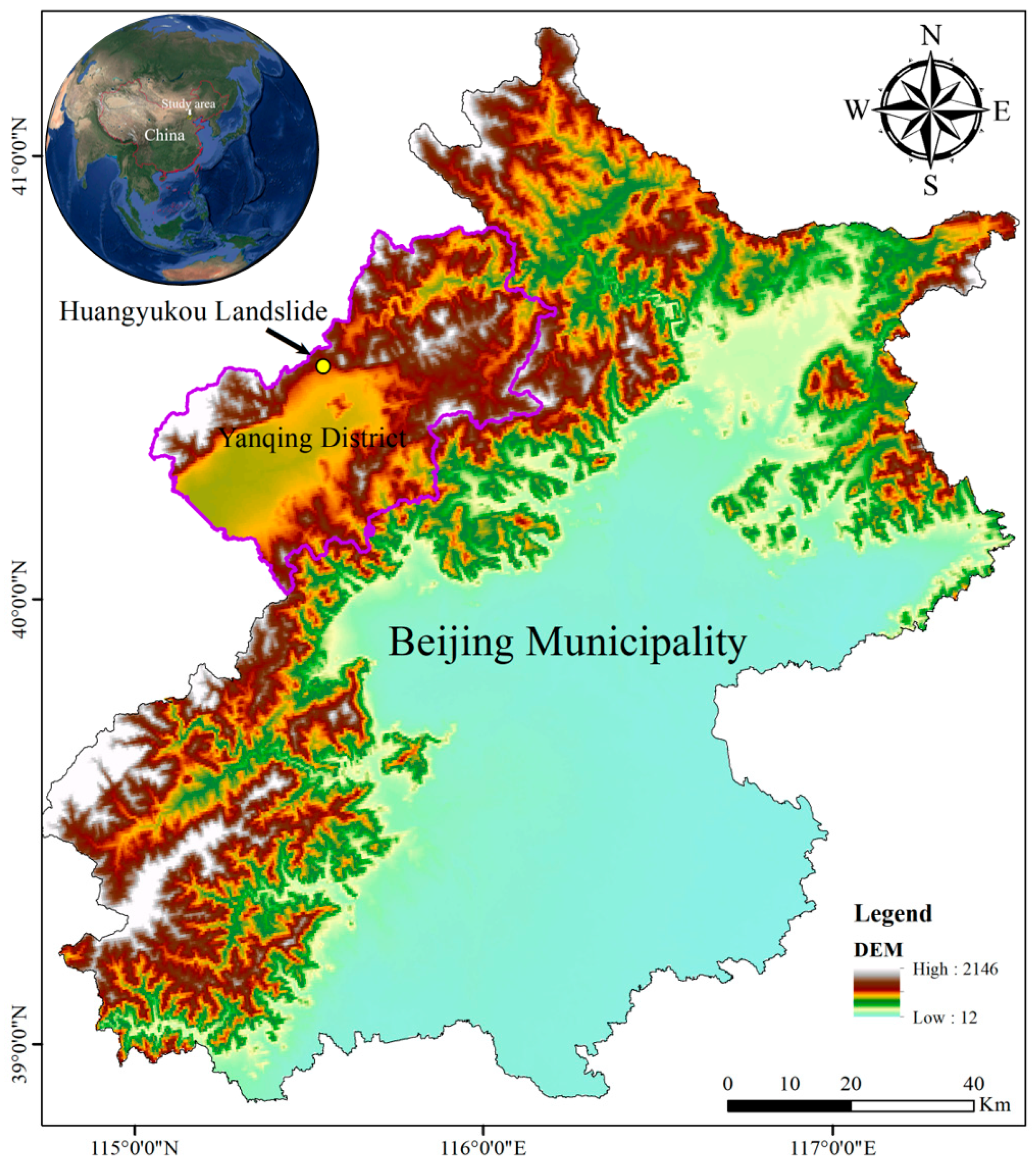
The study area is located on the western slope of the mountain northeast of Huangyukou Village, Jiuxian Town, Yanqing District, Beijing, with geographic coordinates of 116°5′40.5″ E and 40°36′5.6″ N (as shown in Figure 1). This region is situated at the northern edge of the North China Platform and belongs to the central section of the Yanshan fold belt. Since the Archaean, it has undergone multiple tectonic movements and stages of geological evolution, resulting in a complex geological background. The stratigraphy of the study area mainly consists of Archaean metamorphic rocks, dolostone, shale, and Quaternary cover layers. These rocks are characterized by hard lithology, high brittleness, and well-developed joints and fractures, which provide the material foundation for the development of geological hazards.

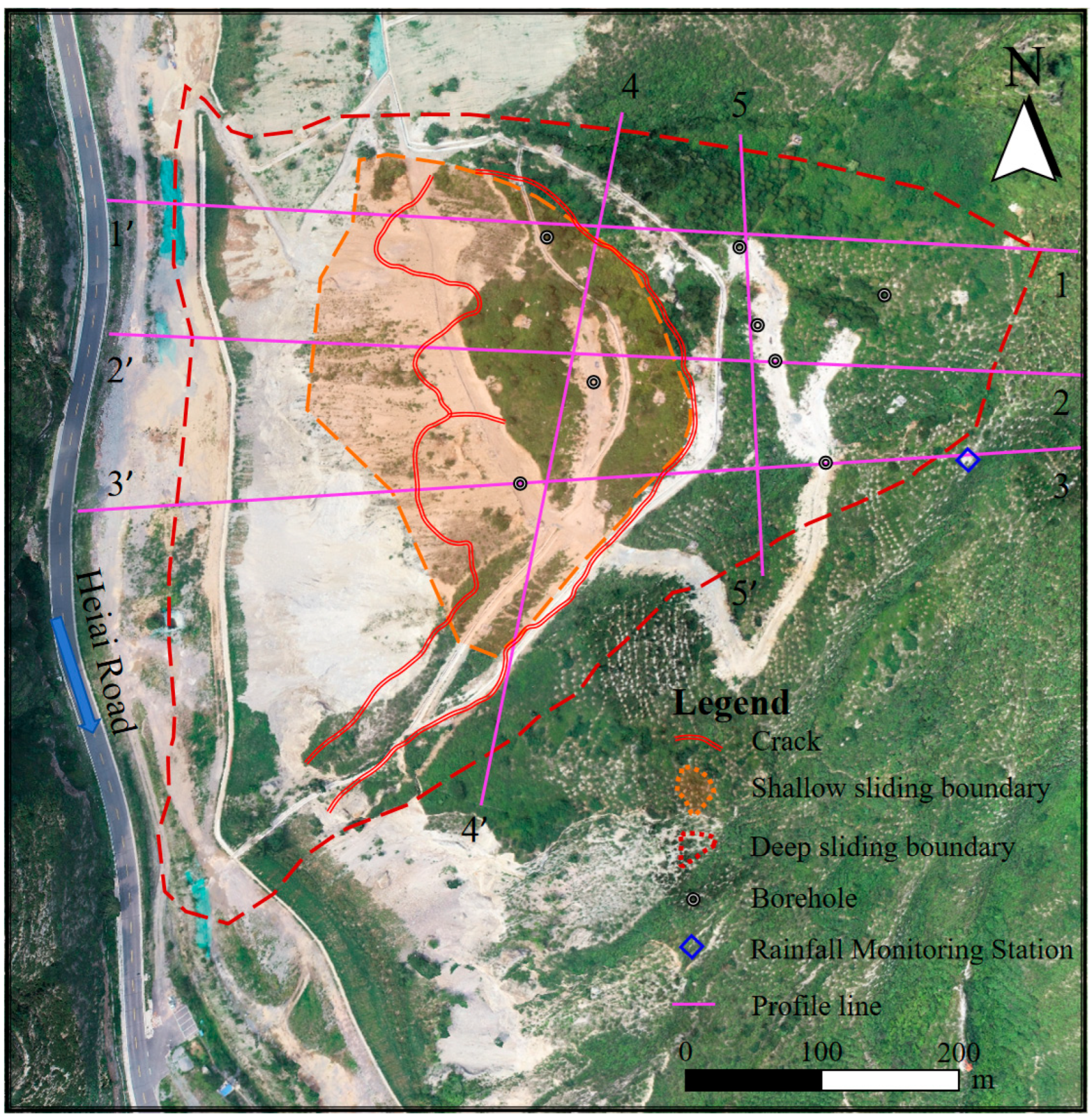
Figure 2 illustrates the topographic and geological features of the research area, focusing on the landslide site. The boundaries of the shallow and deep sliding zones are marked with red and orange dashed lines, respectively, while purple lines indicate profile lines for further investigation. Boreholes, represented by circles, are spread across the area for geological sampling. Rainfall monitoring stations are shown as blue diamonds. The nearby Heiai Road is displayed along the western side of the map. This layout helps analyze the spatial distribution of landslide features and related geophysical factors, offering a comprehensive understanding of the area’s risk and environmental conditions.

From a tectonic perspective, the fault structures in the study area are well developed, primarily consisting of east–west and north–northeast trending faults, followed by northeast and northwest trending faults. These faults of different orientations intersect and form fracture zones and tectonic weak planes, further reducing the geotechnical strength of the landslide mass. Additionally, the fractures and fractured zones provide pathways for rainwater infiltration, exacerbating the impact of rainfall on slope stability. The study area features typical low mountain and hilly terrain, with a slope direction of 270°. The slope gradient is gentle at the top and steep at the bottom, ranging from 20° to 45°. The elevation at the rear of the landslide is approximately 770 m while the front is around 640 m, with a relative elevation difference of about 130 m, indicating significant undulations in the slope terrain. The stratigraphic structure of the landslide mass includes a shallow Quaternary cover layer (26 m thick), a middle weathered rock layer (limestone, 10–15 m thick), and a deep, intact limestone layer (buried at depths of 16 to 30 m).

Regarding groundwater conditions, the study area mainly contains bedrock fissure water and Quaternary loose pore water. Bedrock fissure water is primarily found in dolostone, with well-developed karst fissures. Atmospheric precipitation and surface water replenish the fissure water through vertical infiltration. Quaternary pore water is mainly found in the valley areas at the foot of the landslide, with the aquifer consisting of sand, gravel, and cobbles. The water yield is uneven and the recharge sources include atmospheric precipitation infiltration and lateral replenishment from mountain runoff.

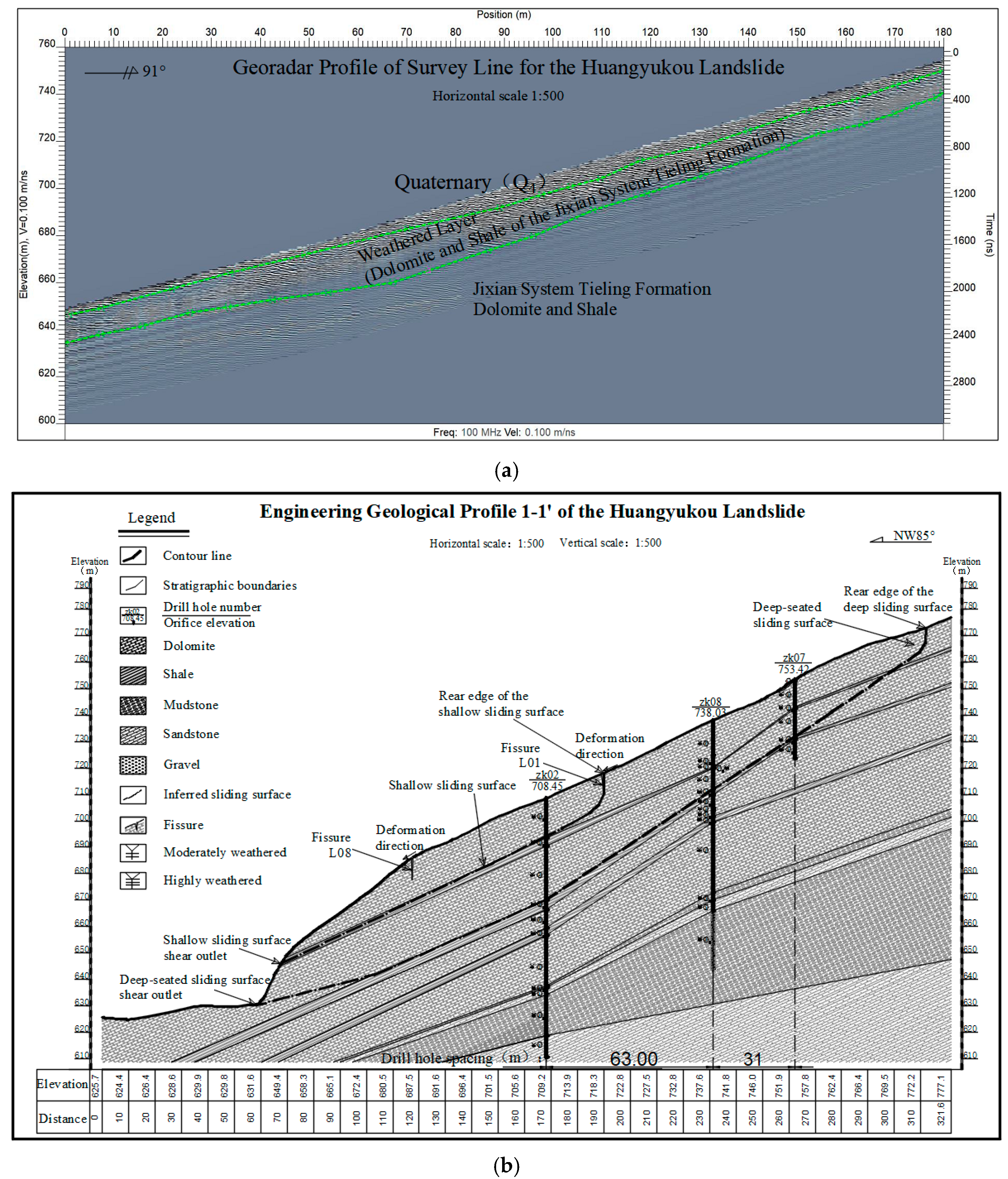
To investigate the subsurface structure and potential slip surfaces of the Huangyukou landslide, a reflected wave ground-penetrating radar profile was obtained. The mode of failure is traction-type. The threatened objects include the channel below, Hei’ai Road, and the inspection station. A geological radar profile was conducted at the Huangyukou landslide, with a length of 180 m and an azimuth of 91°. The surface exposes Quaternary deposits and the bottom of the landslide reveals dolostone and shale. Based on the results of the geological radar, it can be observed that the shallow layers exhibit multiple reflection interfaces with large amplitude variations, uneven waveforms, and significant chaotic reflections. The middle layers show fewer interfaces and the deep layers have relatively few reflection interfaces with uniform waveforms and minimal chaotic reflections. Based on the physical properties and geological conditions, it is inferred that the shallow layer consists of a Quaternary cover layer with a thickness of 2 to 6 m; the middle layer is a weathered layer (limestone) with a thickness of 10 to 15 m; and the deep layer consists of intact limestone with a burial depth ranging from 16 to 30 m. The geological radar results did not show any significant fault or fracture zones. Considering the stratigraphic attitude and field conditions, the Quaternary cover layer and weathered layers are highly susceptible to landslides.

The slope where the landslide is located has an azimuth of 270°, with a gentle upper section and a steep lower section. The natural slope gradient ranges from 20° to 45°. The front edge of the landslide is a steep scarp, 5 to 10 m in height (as shown in Figure 3). The elevation at the rear of the landslide is approximately 770 m while the front edge is about 640 m, with a relative elevation difference of approximately 130 m. The terrain of the slope is highly undulating. Field investigations reveal that the landslide hazard is located on a natural rock slope, with the lithology consisting of dolostone and shale from the Jixian Formation Tieling Group. At some exposed bedrock sites, there are local debris piles. Two potential landslide surfaces have been identified: a shallow landslide and a deep landslide. The shallow landslide has an axial length of 160 m, an average width of 180 m, and an average thickness of 12 m, with a volume of approximately 34.5 × 10⁴ m³, classifying it as a medium-sized landslide. The deep landslide has an axial length of 220 m, an average width of 205 m, and an average thickness of 18 m, with a volume of approximately 79.2 × 10⁴ m³, also classifying it as a medium-sized landslide.

In the landslide area, the thickness of Quaternary residual and colluvial deposits ranges from 0.6 to 4 m. The material composition is primarily silty clay and clayey silt, which are easily slip-prone soils, susceptible to shallow sliding. The bedrock consists of alternating layers of dolomite and shale, with the shale being relatively fractured and low in strength. The contact surface between the dolomite and shale provides favorable conditions for the formation of the landslide slip zone.

At the top of the survey area, there are structurally developed planes with varying directions and scales. Their different combinations form various types of rock mass structures. The strength of these structural planes is significantly lower than that of the intact rock and these structural planes are crucial factors controlling the occurrence of landslides on the slope. The weathered rock layer at the Huangyukou landslide site, identified through ground-penetrating radar interpretation, is approximately 10–15 m thick and lies beneath a 2–6 m Quaternary cover. The radar profile reveals strong amplitude variations, irregular waveforms, and chaotic reflections in this middle section, which indicate significant heterogeneity and discontinuity. Based on these characteristics and in accordance with the ISRM classification system, the weathered limestone is classified as moderately weathered. This level of weathering suggests a notable reduction in strength and increased permeability, both of which are critical in influencing infiltration behavior and slope stability during heavy rainfall events.

The rainfall in the study area plays a critical role in influencing landslide susceptibility. During the rainy season, from July to August, heavy and prolonged rainfall infiltrates through rock fractures, softening fracture surfaces and generating pore water pressure within the fractures. This increases the gravitational load on the slope, reduces cohesion, and accelerates deformation and failure of the rock mass. The region’s monsoon climate results in uneven rainfall distribution across years and seasons, with intense rainfall concentrated in the rainy season. This pattern, coupled with high-intensity rainfall, significantly impacts the stability of the slope, particularly during the flood season, when rainfall aligns with high rainfall centers and corresponding mountain peaks.

Human engineering activities, such as mining, unload at the foot of the slope, providing a free face for landslide formation and displacement, which facilitates the occurrence of landslides. Long-term mining, excavation at the foot of the slope, and the development of dolomite, shale, and joint fractures, with high weathering and low rock strength, alter the stress balance of the slope. Excavation at the front edge of the landslide hazard forms a free face, while tension at the rear edge forms two parallel north–south fractures. From a morphological perspective, the slope has been cut into three steps from top to bottom.

3. Methodology

3.1. Engineering Geophysical Survey

The use of geophysical methods can accurately identify subsurface features, such as fractures, cover layer thickness, and weathered bedrock zones, helping to assess slope stability. Compared to traditional drilling methods, geophysical methods are more cost effective and efficient, especially in areas that are difficult to access directly [18]. In this study, two geophysical methods, ground-penetrating radar (GPR) and high-density electrical methods, were used during the landslide investigation. The GPR utilized the EKKO ground-penetrating radar from SSI (Yellowknife, NT, Canada), equipped with an antenna frequency of 100 MHz. Point measurements were conducted with 65,536 stacking repetitions, a sampling duration of 1000 ns, a point distance of 0.3–0.5 m, and a detection depth of 45 m. The dielectric constant was 0.1 m/ns, with a transmitter–receiver antenna spacing of 0.5 m. The high-density electrical method employed the DUK-4 series high-density electrical measurement system produced by Zhongdi Instruments (Chongqing) Co., Ltd. (Chongqing, China). The measuring device used was the Wenner device, with 120 electrodes, measurement point spacing of 1–2 m, and a detection depth ranging from 20 to 40 m.

Through the GPR and high-density electrical methods, the location, attitude, and properties of the fracture zones were detected. The tensile cracks at the rear edge and the 20 bulging cracks at the front edge, along with their location, attitude, and filling conditions, were investigated. The thickness of the cover layer was determined and the bedrock surface morphology was identified. The weathered bedrock zone was divided and its thickness was measured. The stratigraphic structure of the landslide mass, the lithological contacts, and the thickness of the landslide deposit were explored to define the shape of the accumulation bed. The main methods used were high-density electrical methods and GPR, with a design of 450 m for the high-density electrical method and 3000 points for the GPR.

3.2. The Construction of Design Rainfall Intensity Curves for Different Return Periods

The rainfall intensity calculation formula is shown in Equation (1):

$$q={\displaystyle \frac{167A_1(1+clgP)}{{(t+b)}^n}}$$

(1)

In this formula, $q$ represents the design rainfall intensity, with units of liters per second per hectare; $P$ is the design return period of the heavy rainfall, measured in years; $t$ is the rainfall duration, measured in minutes (min); and $A_1$, $c$, $b$, and $n$ are empirical parameters representing rainfall intensity, rainfall variation, rainfall duration correction, and rainfall attenuation index, respectively. These parameters are selected based on the rainfall characteristics of the study area. The final rainfall calculation formula for the study area is shown in Equation (2). $P$ ranges from 2 to 100 years, meaning it can be used to calculate the rainfall intensity for events ranging from a 2-year to a 100-year return period:

$$q=\left\{\begin{array}{c}{\displaystyle \frac{1558(1+0.955lgP)}{{(t+5.551)}^{0.835}}}, 1 \mathrm{m}\mathrm{i}\mathrm{n}\le t\le 5 \mathrm{m}\mathrm{i}\mathrm{n}\\ \\ {\displaystyle \frac{2719(1+0.96lgP)}{{(t+11.591)}^{0.905}}}, 5 \mathrm{m}\mathrm{i}\mathrm{n}\le t\le 1440 \mathrm{m}\mathrm{i}\mathrm{n}\end{array}\right.$$

(2)

3.3. The Hydrological Model Considering Runoff–Infiltration Coupling

This study employs a GPU-accelerated parallel framework to simulate the infiltration and surface runoff processes of unsaturated soil slopes under rainfall, using a hydrological model that considers runoff–infiltration coupling. This study investigates surface runoff variations caused by topographic changes, surface–groundwater interactions, and groundwater infiltration processes in the soil. The hydrological model accounts for two-dimensional surface runoff and three-dimensional unsaturated subsurface infiltration processes. The surface runoff is modeled using the depth-averaged flow equation, while the subsurface infiltration is based on the Richards equation.

The depth-averaged flow equation for surface runoff consists of the continuity (mass conservation) equation and momentum equations in two directions. The continuity equation for surface runoff can be expressed as:

$${\displaystyle \frac{\partial h}{\partial t}}+\nabla ·(\overrightarrow{v}h)+q_e+q_r=0$$

(3)

where $h$ represents the surface water depth; $t$ represents time; $\overrightarrow{v}$ represents the depth-averaged velocity vector; $q_e$ represents the exchange flux between the surface and subsurface; $q_r$ represents the source (sink) terms, such as rainfall or evaporation; and $\nabla$ represents the vector differential operator used to express the divergence of flow.

$$S_{f,i}=S_n$$

(4)

$$S_{f,i}=\partial H/\partial x_i$$

(5)

$$S_n=\sqrt{{(\partial H/\partial x)}^2+{(\partial H/\partial y)}^2}$$

(6)

$$H=h+z$$

(7)

The momentum equation for surface runoff can be expressed as: where $S_{f,i}$ is the friction slope and $i$ represents the x or y direction; $S_n$ is the surface slope; $H$ is the water surface elevation; and $z$ is the ground surface elevation.

The relationship between water depth and flow can be established using Manning’s coefficient equation:

$${\overrightarrow{v}}_i=-{\displaystyle \frac{h^{2/3}}{n_b\sqrt{S_n}}}{\displaystyle \frac{\partial H}{\partial x_i}}=-{\displaystyle \frac{D}{h}}{\displaystyle \frac{\partial H}{\partial x_i}}$$

(8)

$$D={\displaystyle \frac{h^{5/3}}{n_b\sqrt{S_n}}},D=\left|S_n\right|>S_{min} and h>h_{min}$$

(9)

where $D$ is the diffusion coefficient, which controls the wet-dry boundary and is 0 when the above condition is not met; $n_b$ is the Manning roughness coefficient; $S_{min}$ is used to define the range for the diffusion coefficient $D$, and $h_{min}$ is the threshold to define whether the surface has water.

Substituting Equations (8) and (9) into Equation (3) yields Equations (4) and (10), which represent the final governing equations used for surface runoff:

$${\displaystyle \frac{\partial H}{\partial t}}={\displaystyle \frac{\partial }{\partial x}}(D{\displaystyle \frac{\partial H}{\partial x}})+{\displaystyle \frac{\partial }{\partial y}}(D{\displaystyle \frac{\partial H}{\partial y}})-q_e-q_r$$

(10)

In the calculation program, the boundary condition conversion method is used to solve the coupling process between surface water and groundwater, i.e., the boundary condition type (Neumann or Dirichlet boundary) at the surface–subsurface interface is changed according to the surface water accumulation status. The Neumann boundary represents a fixed flux boundary condition, corresponding to infiltration or outflow, with the flux magnitude equal to rainfall or evaporation. The Dirichlet boundary represents a fixed head boundary condition, which is activated when the surface node reaches the saturation (or ponding) threshold. The infiltration and exfiltration processes are controlled by soil parameters. The boundary condition conversion method does not require introducing new parameters to represent the exchange process or interface properties, while maintaining the continuity of exchange flux and pressure head at the interface.

The depth-averaged equation for surface runoff and the Richards equation for subsurface infiltration are both solved using the Alternating Direction Implicit (ADI) method. This method only requires a tridiagonal linear matrix for computation, which has the advantages of simpler computation and faster solution compared to the fully implicit method. As the problem dimension increases, the ADI method requires less computational effort and offers better stability than the fully implicit method.

3.4. Deformation Analysis Method of Slopes Under the Rainfall Hydrological–Geotechnical Coupling Effect

The analysis of hydrological processes under rainfall includes the combined effects of surface runoff and subsurface infiltration [19,20]. Subsurface infiltration is calculated based on the Richards equation to model the infiltration process of rainwater in unsaturated soil. If a slope unit reaches saturation, the depth-averaged equation is used to solve the surface runoff process. The coupling effect between runoff and infiltration is calculated through the water exchange amount at the slope unit. The simulated hydrological results, including the soil moisture content and the distribution of water heads, are applied as initial conditions to the corresponding 3D geological model. Due to differences in moisture content and water head, the particle density, permeability, and strength parameters change. Additionally, under extreme rainfall conditions, the erosion effect near the surface particles caused by runoff needs to be considered. After mapping the hydrological results to the geological model, the stability analysis of the slope model is carried out under the combined influence of multiple factors.

For the 3D model, after being influenced by the soil moisture content and permeability transmitted from the hydrological model units, the particle information changes in four aspects: bulk density, permeability, erosive force, and soil strength.

As rainwater infiltrates, the infiltration depth in the unsaturated soil continues to increase and the water content within the soil increases, leading to an increase in bulk density:

$$m_P={\rho }_P{V}_P+{\displaystyle \frac{\theta }{{\theta }_S}}{\rho }_w{V}_P\varphi$$

(11)

where $m_P$, $V_P$, and ${\rho }_P$ are the particle mass, volume, and density, respectively; ${\rho }_w$ is the density of water, taken as 1000 kg/m³; and $\theta$, ${\theta }_S$, and $\varphi$ are the soil moisture, maximum water content, and porosity, respectively.

When the saturation of the unsaturated soil reaches 80% or higher, the soil is considered to be nearly saturated and the water infiltration process in the soil is influenced by permeability. The infiltration force can be calculated based on the water head difference between adjacent units:

$$f_{seep,i}={\rho }_{w}g∆H{S}_i$$

(12)

where $g$ denotes gravitational acceleration; $∆H$ represents the total water head difference between adjacent units; $i$ represents a direction (x, y, or z); and $S_i$ represents the cross-sectional area of the unit. When $i$ represents the x direction, then $S_i$ = Δy × Δz. The direction of the permeability force is from high water head units to low water head units.

The surface runoff process can be equivalently considered the erosion process caused by water flow in a river channel. The water erosion force τ on any unit can be expressed as:

$$\tau ={\rho }_{w}gR{S}_{slope}$$

(13)

where $R$ represents the hydraulic radius, mainly influenced by the unit cross-sectional width $W$ and water depth $h$, and $S_{slope}$ is the slope of the unit, indicating the direction from high to low, corresponding to the direction of the erosion force:

$$R={\displaystyle \frac{Wh}{W+2h}}$$

(14)

The Fredlund model, characterized by its multiple parameters and continuous functional form, demonstrates high accuracy and broad applicability in fitting particle size distribution curves and predicting soil water characteristic curves [19]. The shear strength of unsaturated soil is usually described using the Fredlund form:

$$\tau =c_0^{\prime }+\left(\sigma -u\right)tan{\phi }^{\prime }+(u_a-u_w)tan{\phi }^b$$

(15)

where $c_0^{\prime }$ is the effective cohesion; $\sigma$ is the normal stress; and $u_a$ and $u_w$ represent the pore gas pressure and pore water pressure, respectively. During the calculation process, the influence of gas is ignored and $u_a$ = 0 is simplified. When the soil reaches saturation, the matric suction becomes zero and, thus, the third term is zero. When the soil is still unsaturated, it can be considered cohesion and the total cohesion of the soil can be expressed as:

$$c\prime =c_0^{\prime }+(u_a-u_w)tan{\phi }^b$$

(16)

Clearly, as the moisture content increases, the total cohesion of the soil continuously decreases. Based on the soil–water characteristic curve of the soil, the matric suction corresponding to different moisture contents can be directly determined and, thus, the relationship between total cohesion and moisture content can be obtained.

3.5. Slope Stability Analysis Methods

In SRM, by defining the reduction factor $R_f$, the strength parameters continuously decrease during the calculation process. The reduced effective internal friction angle ${\phi }_f$ and effective cohesion $C_F$ are obtained, from which the reduced shear strength ${\tau }_{fF}$ can be calculated:

$${\phi }_f={tan}^{-1}((tan\phi )/R_f))$$

(17)

$$C_F=C/R_f$$

(18)

$${\tau }_{fF}=C_F+\sigma tan{\phi }_f$$

(19)

In the calculation process, the reduction factor $R_f$ is gradually increased to reduce the shear strength of the slope’s soil and rock mass until the entire slope gradually deforms, becomes unstable, or fails. Here, the non-convergent state is chosen as the criterion for slope instability. If the unbalanced forces do not converge, the corresponding $R_f$ at this point is taken as the slope stability factor (FOS).

4. Results and Discussion

4.1. Calculation of Rainfall Intensity Curves

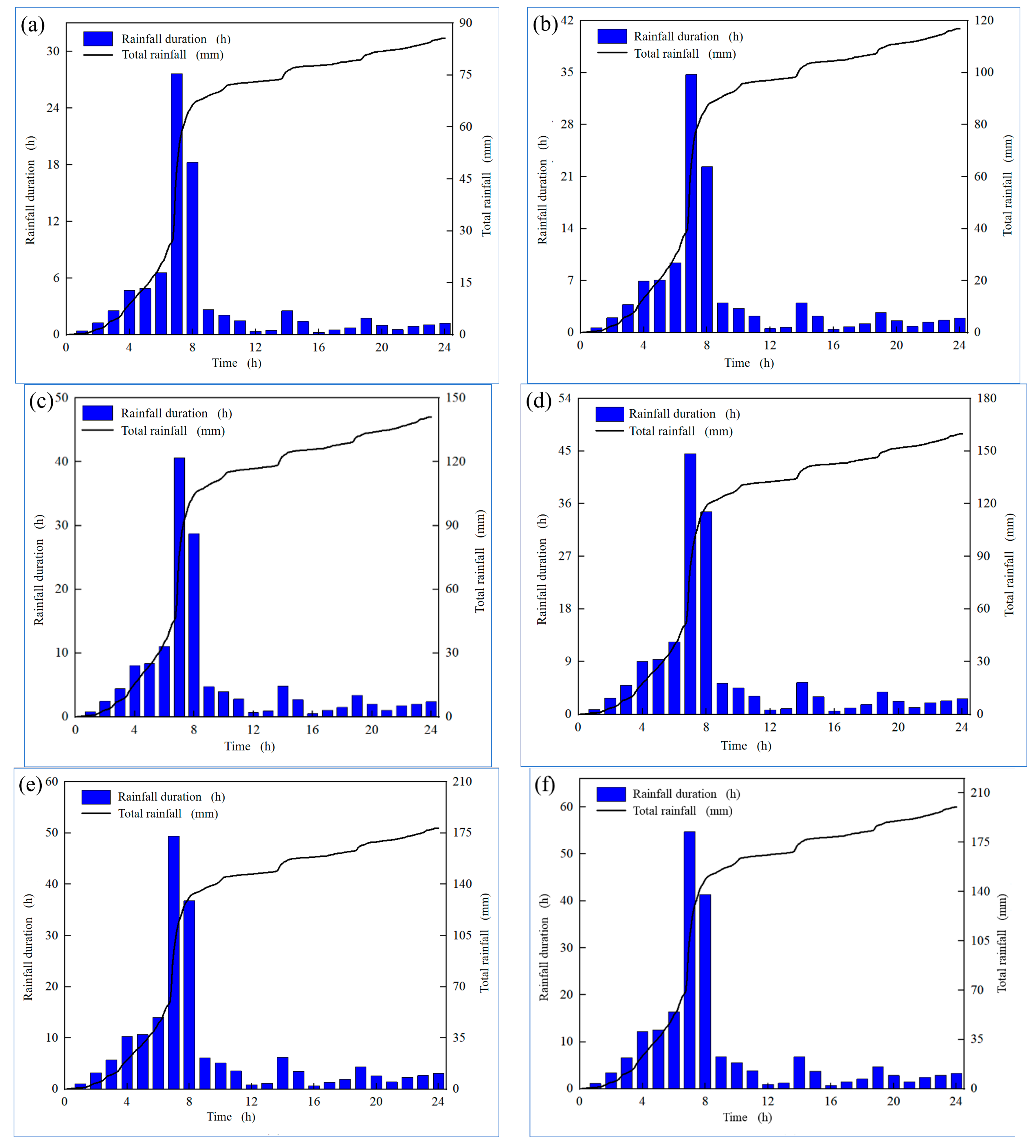
The rainfall intensity for durations ranging from 1 to 1440 min can be calculated using this formula. Combined with the design rainfall pattern, rainfall event data with a minimum time interval of 5 min and a total duration of 1440 min can be obtained (the design rainfall pattern for the study area refers to the standard) [21].

Rainfall event data for different return periods (5 years, 10 years, 20 years, 30 years, 50 years, and 100 years) in the study area were selected and the duration curves of rainfall were plotted, as shown in Figure 4.

4.2. Stability Analysis of the Typical Landslide Profile

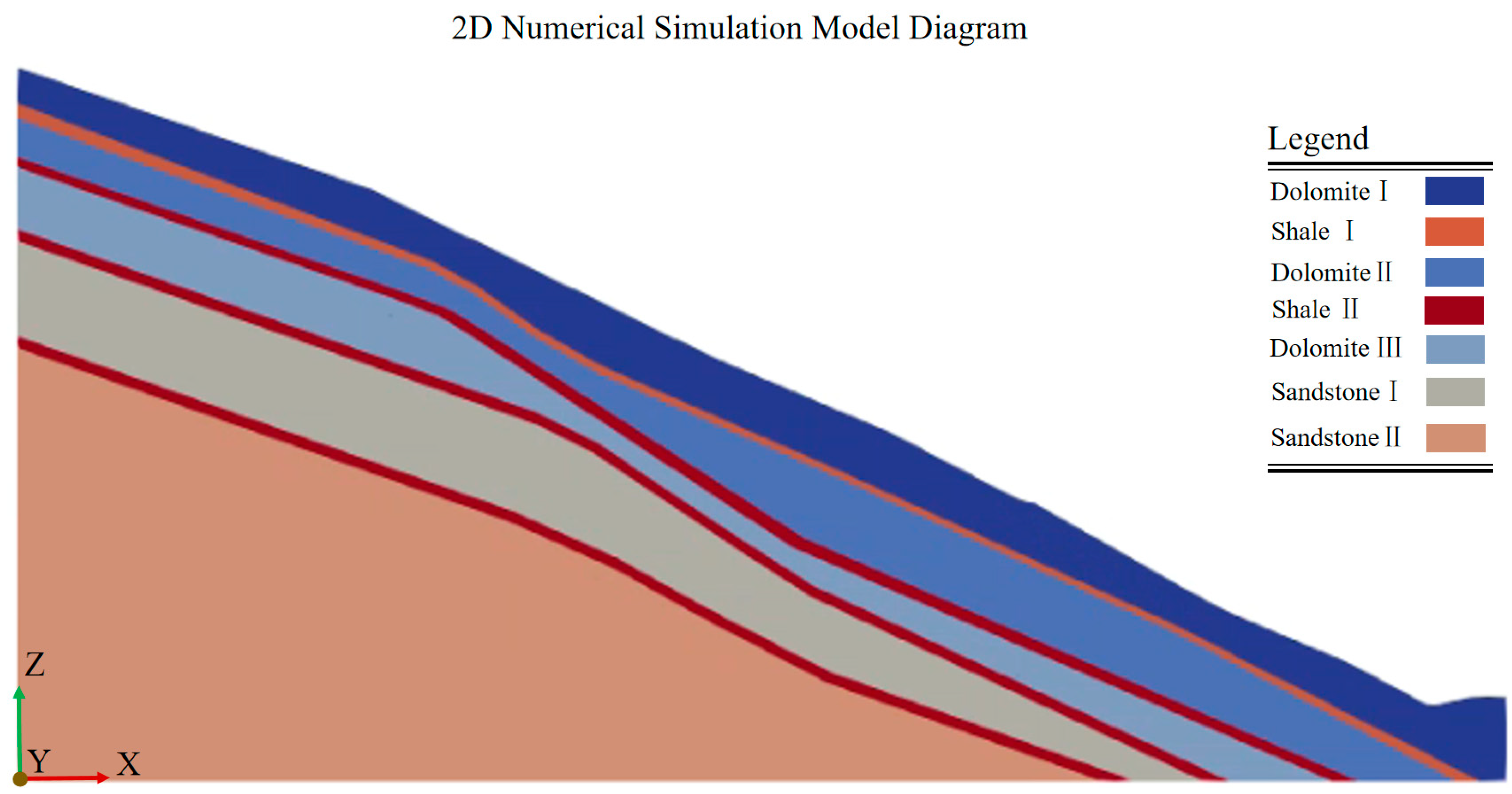
Based on the landslide engineering geological characteristics described earlier, and referencing field survey data and geological profile diagrams, a two-dimensional numerical model of the landslide was established (Figure 5). Stability calculations and analysis were performed using the discrete element method (DEM) module of CoSim, with the model consisting of 18,335 blocks.

The geotechnical parameters of the soil and rock mass were obtained through laboratory tests on undisturbed samples from the boreholes. Combined with the engineering geological characteristics and lithological composition of the landslide, the material parameters used in the calculation and simulation are shown in

Table 1. Landslide material parameters table of hydrological model.

Material	Elastic Modulus (GPa)	Poisson’s Ratio	Static Friction Angle (°)	Dynamic Friction Angle (°)	Normal Cohesion (kPa)	Shear Cohesion (kPa)	Density (kg/m3)
Dolomite 1	2	0.2	40	30	1800	1500	2400
Shale 1	1	0.2	30	20	480	400	2300
Dolomite 2	2	0.2	40	30	2400	2000	2400
Shale 2	1	0.2	30	20	600	500	2300
Dolomite 3	2	0.2	40	30	3600	3000	2400
Sandstone 1	2	0.2	40	30	6000	5000	2400
Sandstone 2	2	0.2	40	30	6000	5000	2400

. The dolostone layer, shale layer, and sandstone layer are all modeled using a cohesive–frictional material constitutive model.

To determine the stability factor of the landslide in its natural state, the displacement information of the block bodies at key positions on the slope, namely, the crest (P1), mid-slope (P2), and toe (P3), was monitored under different reduction factors. Additionally, the rupture situation of the slope was observed, including the number of tensile and shear cracks under various reduction factors. Figure 6 shows the displacement of P1, P2, and P3 as a function of the increase in Rf and Figure 6b shows the change in the number of cracks with increasing Rf. When Rf is less than 1.12, the increase in displacement and crack number is relatively slow and the slope’s displacement and rupture develop gradually. As Rf reaches 1.12, the increase in displacement and crack number accelerates, marking the turning point of the curve. At this point, some of the cracks in the slope become through-going and the overall displacement increases. When Rf exceeds 1.12, displacement and crack numbers increase rapidly, indicating that the cracks have fully propagated and the slope has failed and become unstable. Therefore, the stability factor of the landslide in its natural state can be defined as 1.12.

The landslide mass consists of dolomite, interspersed with thin layers of shale. Due to excavation at the slope toe, a creep deformation towards the free face is generated and an interlayer shear occurs along the soft–hard contact surfaces between the shale and dolomite. The lower shear strength of the shale, with a cohesion of 40 kPa, compared to the dolomite, facilitates the interlayer shear. When the reduction factor is 1.06, under the effect of the self-weight of the slope, sliding initiates at the leading edge, pulling the rear slope and generating tensile cracks. The upper dolomite undergoes shear creep deformation along the shale layers but the overall slope remains stable. As the reduction factor reaches 1.12, landslide deformation intensifies, with significant tensile cracks appearing at the rear of the landslide. The shallow sliding surface becomes continuous, part of the upper dolomite collapses, and the deep sliding surface progressively fails, eventually forming a continuous sliding surface (as shown in Figure 7). The entire landslide mass, influenced by the differential material properties of the dolomite and shale, undergoes deformation and failure, transitioning into an unstable state.

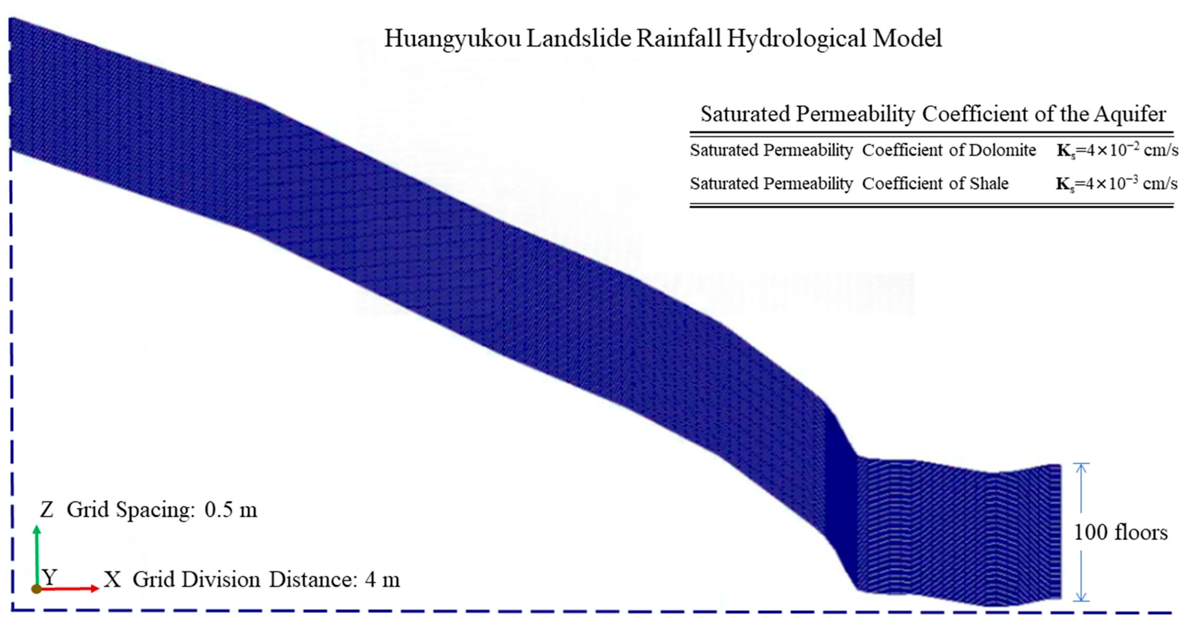
The rainfall calculation model for the Huangyukou landslide surface was generated based on the topological model (Figure 8). In the X direction, the grid is divided with a spacing of 4 m while, in the Z direction, a grid spacing of 0.5 m is used, generating 100 layers of grids. The boundary conditions of the hydrological model are Dirichlet fixed-head no-flow boundary conditions. The Richards equation is solved using the finite element method (FEM) with implicit time integration for handling complex geometries and heterogeneous soil conditions. Boundary conditions include a time-varying Dirichlet fixed head at the top, a no-flow Neumann condition at the bottom, and no-flow conditions at the lateral boundaries, reflecting the model’s symmetry and minimal horizontal seepage.

The upper part of the landslide mass primarily consists of dolomite and shale, with well-developed joints and fractures. The rock is highly fractured and the surface is intensely weathered, making it highly permeable, with a large permeability coefficient. The saturated permeability coefficient for dolomite is set to Ks = 4 × 10⁻² cm/s and, for shale, Ks = 4 × 10⁻³ cm/s. The unsaturated rock and soil in this region are modeled using the van Genuchten model, with the VG model parameters set the same as those for the G109-1# landslide hydrological model in the Mentougou area.

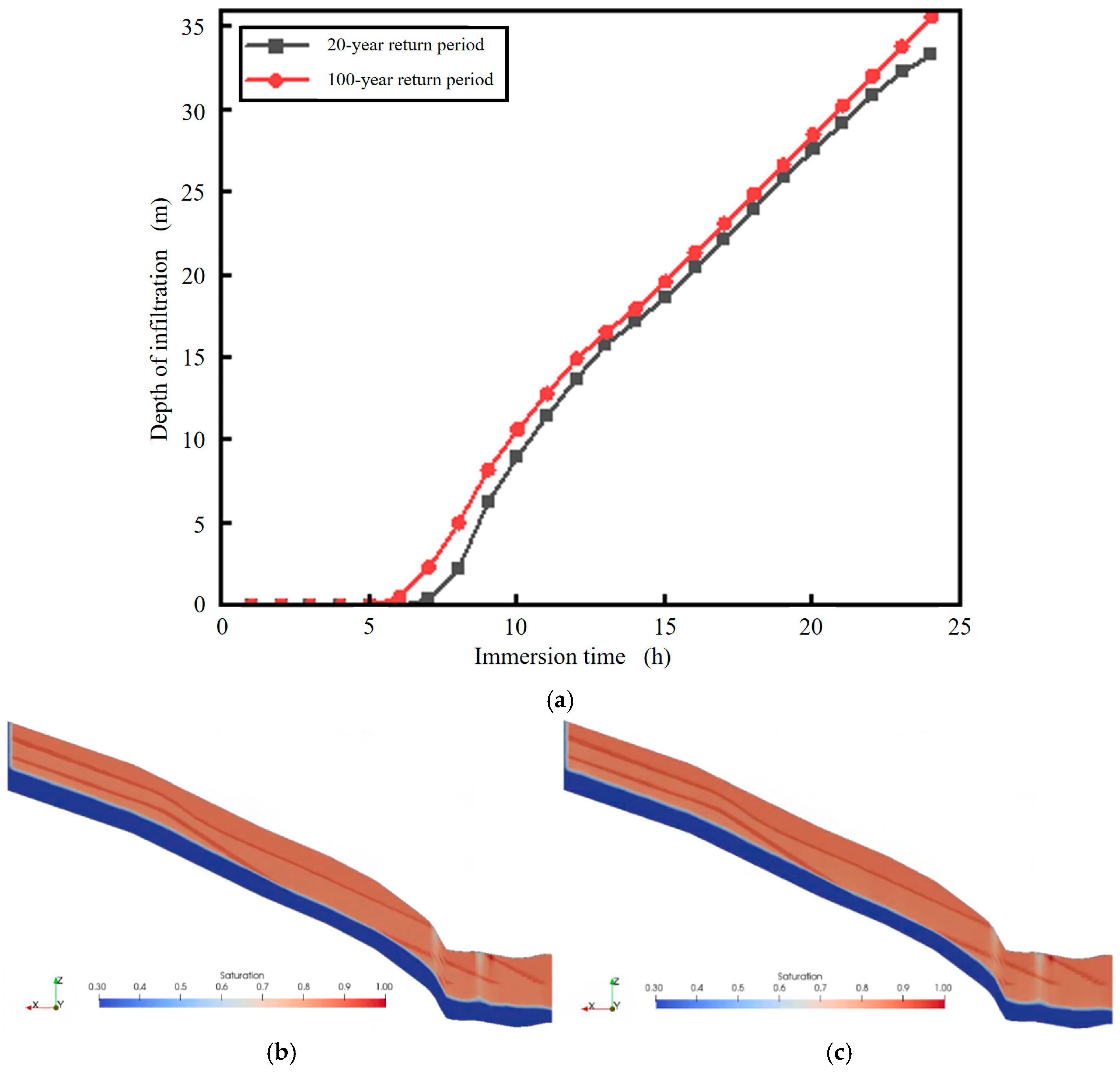
Under 20-year return period rainfall conditions, it is assumed that all the rainwater infiltrates into the slope without generating surface runoff. Under 100-year return period rainfall conditions, part of the rainwater infiltrates into the slope while the rest forms surface runoff. Figure 9 shows the development curves of infiltration depth over time and the saturation distribution of infiltration under both conditions. Due to the high permeability coefficient, the overall infiltration speed is relatively fast. Initially, the soil is relatively dry and the rainwater rapidly infiltrates into the interior with a high infiltration rate. As infiltration progresses, the shallow soil layers approach a near-saturated state and the infiltration peak develops at a stable rate, moving inward at a constant speed. After 24 h of rainfall, the final infiltration depths for the two conditions are 33.3 m and 35.6 m, respectively.

To investigate the stability of the landslide under rainfall conditions, the hydrological results from the model calculated in the previous section, including saturation, water head, and other information, are mapped onto the blocks within the current grid through grid interpolation. The corresponding blocks experience increases in unit weight, body force, and strength reduction. For the 100-year return period scenario, the impact of surface runoff erosion on the upper surface units of the slope also needs to be considered. Based on the above hydrological information, a stability analysis of the landslide under rainfall conditions was conducted.

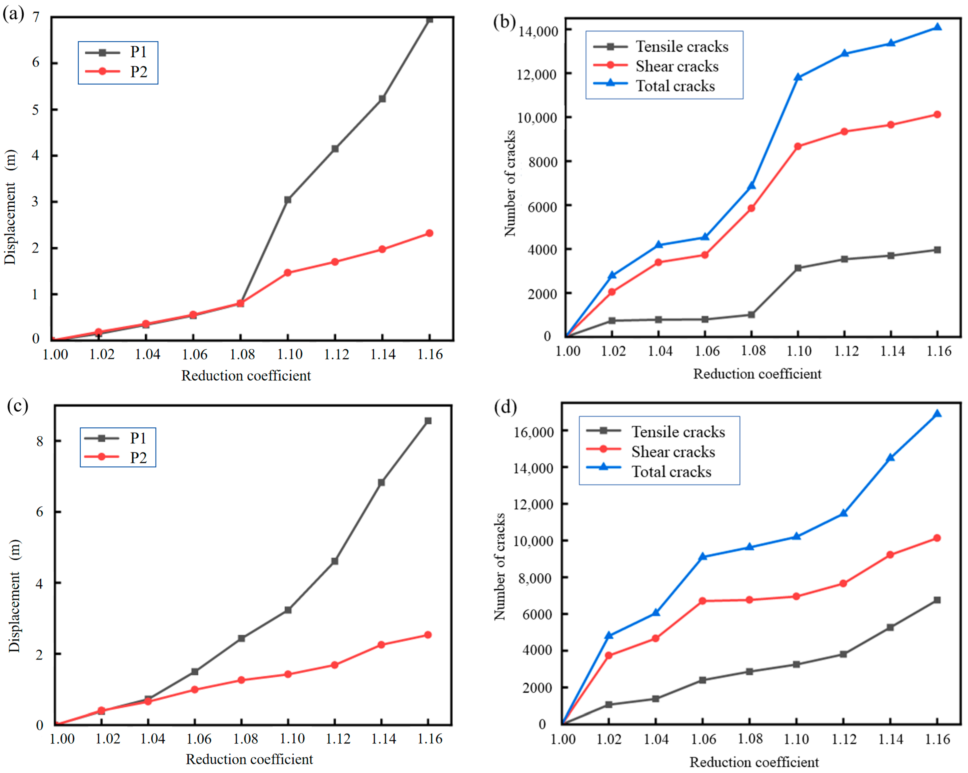
Figure 10 shows the variation of displacement and crack number of key blocks with increasing Rf under different rainfall conditions. Under the 20-year return period rainfall probability, the curve shows a turning point at 1.06, at which the slope becomes unstable. After this point, displacement and crack number rapidly increase so the stability factor of the slope under the 20-year return period is defined as 1.06. Under the 100-year return period rainfall probability, the curve exhibits a sudden change at 1.04, where the cracks in the slope have already become through-going and the slope has entered an unstable failure state. Therefore, the stability factor of the slope under the 100-year return period is defined as 1.04.

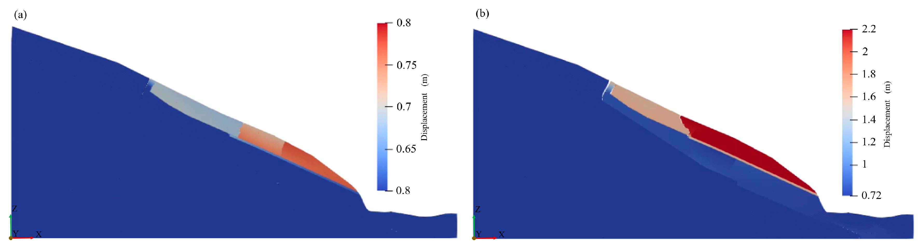
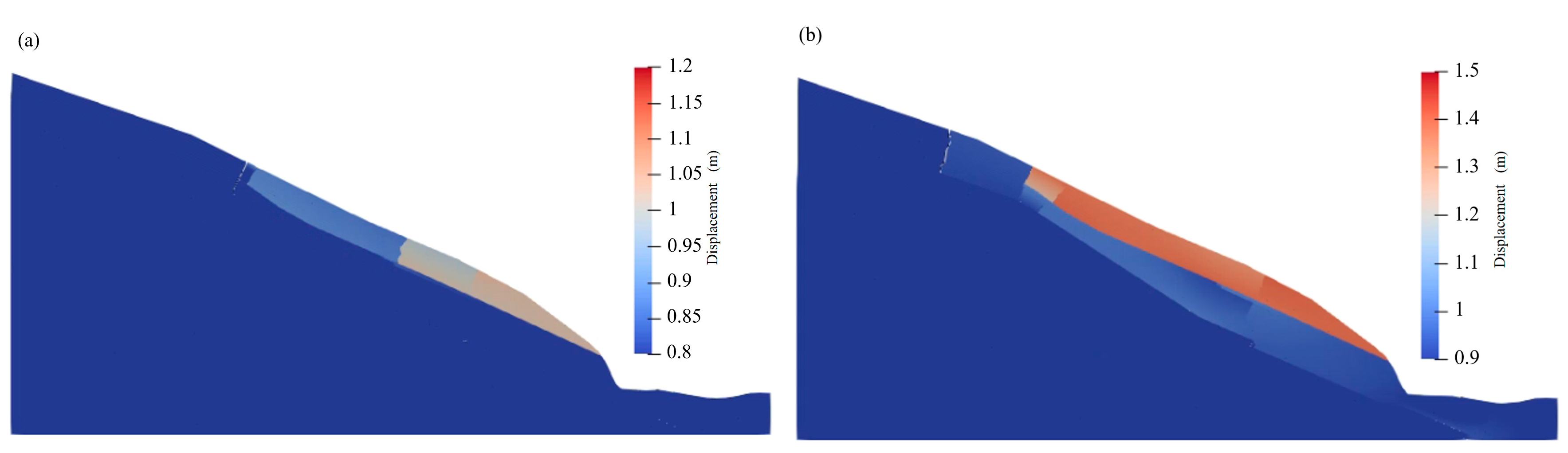
Figure 11 shows the deformation and failure process of the landslide under different rainfall probabilities. The calculations reveal that under rainfall conditions, the upper dolomite and shale of the landslide are more affected, with displacements significantly larger than in the natural state. Under the 20-year return period rainfall conditions, the first layer of shale softens upon water contact, leading to a reduction in strength. Shallow dolomite shows partial tensile cracks and there is a tendency for an interlayer shear along the contact surface of the shale. Under the 100-year return period rainfall conditions, the weakening of the shale strength in the slip zone exacerbates the deformation of the landslide. The slip zone, where sliding occurs due to reduced material strength, is significantly affected by the decrease in shale strength, which facilitates shear failure. As a result, the shallow layers experience localized slumping, mainly due to shear failure that leads to downward movement. Meanwhile, the deep sliding surface becomes progressively unstable, eventually forming a continuous sliding surface, increasing the overall instability of the slope.

The calculated slope stability factor for the 20-year return period is 1.08, which is classified as a yellow warning in the stability alert system, indicating a basic stable state. For the 100-year return period, the slope stability factor is 1.04, which is classified as an orange warning, indicating an unstable state. Based on rainfall process data for different return period rainfalls in the area, a detailed analysis of the slope deformation and failure states for the 20-year and 100-year return periods allows for defining the slope stability factor for a 50-year return period as 1.05, indicating a basic stable state.

4.3. Three-Dimensional Stability Analysis of the Landslide Mass

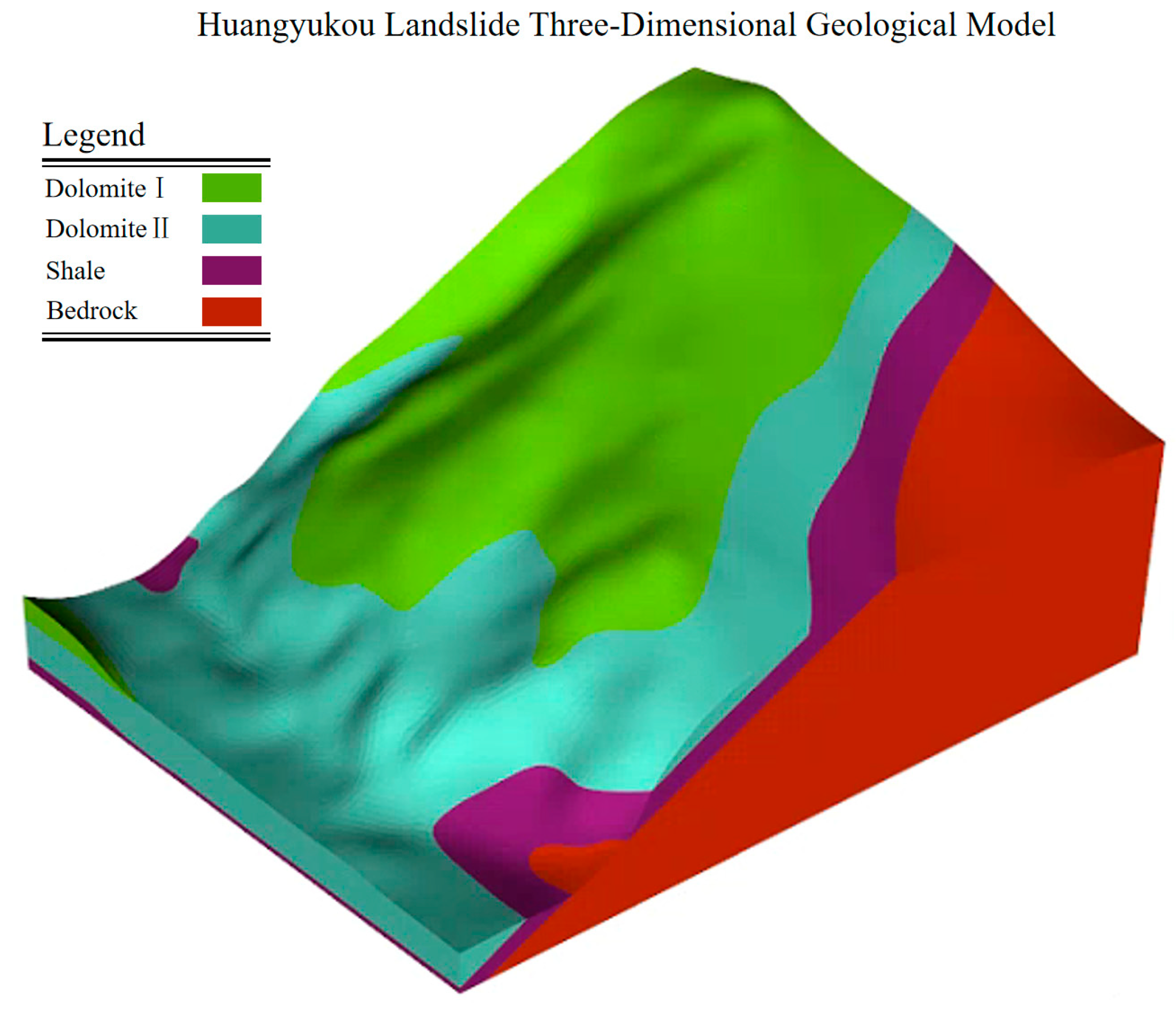
Based on the engineering geological characteristics of the landslide, and referencing field investigation data and geological profile diagrams, a three-dimensional geological and mechanical structural model of the Huangyukou landslide mass was established. Using the contour terrain information of the study area, elevation point cloud extraction was first performed to generate a three-dimensional terrain point cloud for the study area, which was then used to create the terrain surface. Subsequently, based on the positions of various stratigraphic boundaries, profile orientation information, and borehole coordinates from the geological profile diagrams, the stratigraphic layers were established. Finally, the layers of the model were divided into tetrahedral grids. Figure 12 shows the computational model after grid division, with a total of 324,828 elements using four-node tetrahedral units. Stability calculations were conducted using the CoSim discrete element method (DEM) module.

Referring to geotechnical test data for the mechanical parameters of the rock and soil, and combining the engineering geological characteristics and lithological composition of the landslide in Section 4, the material parameters used in the simulation are shown in

Table 2. Landslide material parameters table.

Material	Elastic Modulus (GPa)	Poisson’s Ratio	Static Friction Angle (°)	Dynamic Friction Angle (°)	Normal Cohesion (kPa)	Shear Cohesion (kPa)	Density (kg/m3)
Dolomite	1	0.1	45	35	1200	1200	2400
Shale	1	0.1	25	20	600	600	2400
Bedrock	3	0.1	50	35	7200	6000	2400

. All rock layers are modeled using a cohesive-frictional material constitutive model.

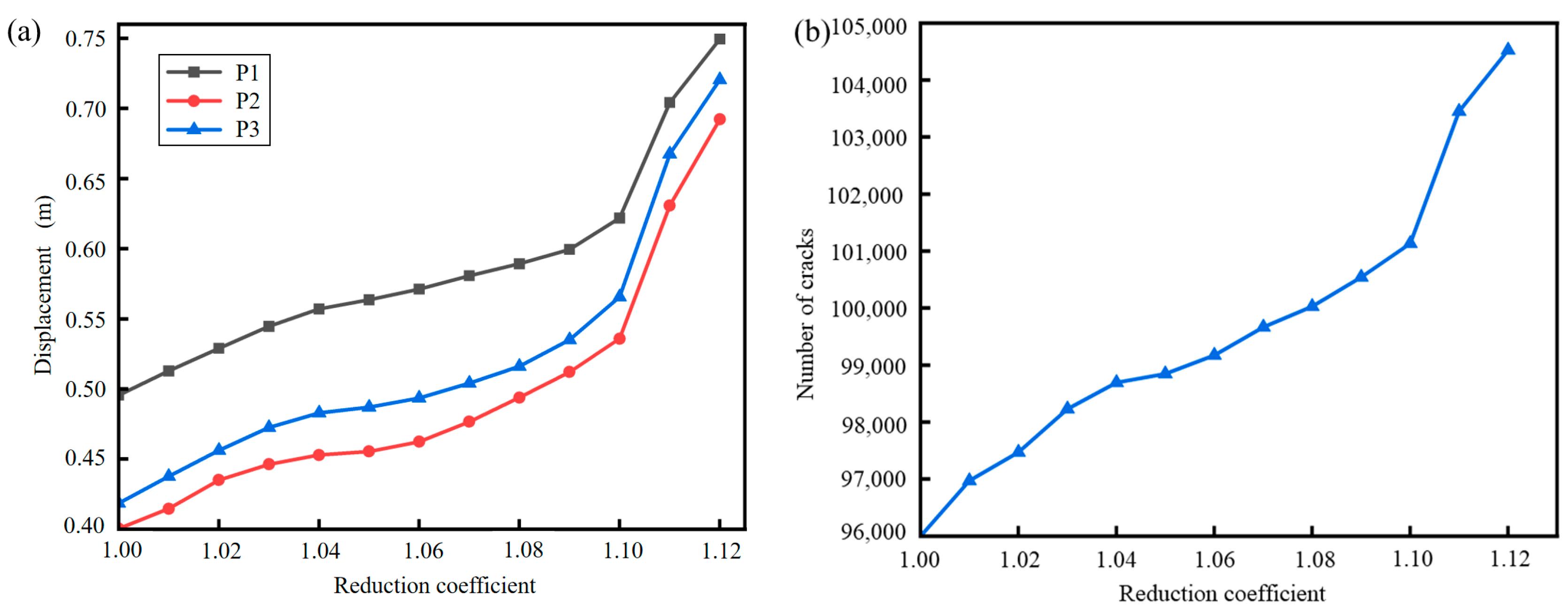
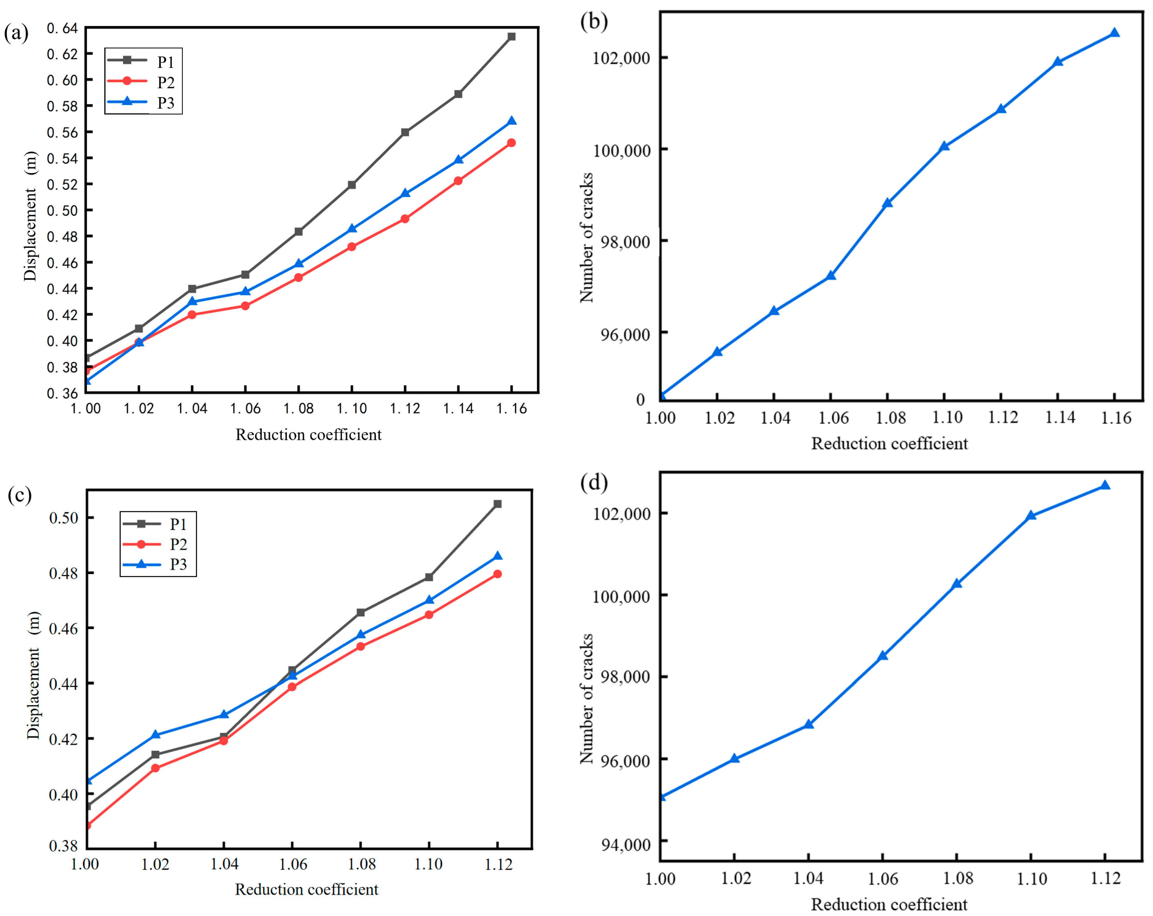
To determine the stability factor of the landslide in its natural state, displacement information of the block bodies at key positions on the slope, namely, the crest (P1), mid-slope (P2), and toe (P3), was monitored under different reduction factors. Additionally, the rupture situation of the slope was observed, including the number of cracks formed. Figure 13a shows the variation in the displacement of P1, P2, and P3 with increasing Rf, and Figure 13b shows the change in the number of cracks with increasing Rf. In the initial stage, the curve has a small slope and the increase in the displacement and crack number is slow, with the displacement and rupture gradually developing. When Rf reaches 1.10, the increase in the displacement and crack number accelerates suddenly, marking a turning point in the curve. At this point, some cracks in the slope become through-going and the overall displacement increases. As Rf continues to increase, displacement and crack number increase rapidly, indicating that the cracks have fully propagated and the slope has failed and become unstable. Therefore, the stability factor of the landslide in its natural state is defined as 1.10.

Figure 14 shows the deformation and failure state of the landslide mass. The landslide mass consists of dolomite interspersed with thin layers of shale. In the natural state, under the influence of self-weight and the free face, the front edge of the uppermost dolomite first experiences creep deformation towards the free face. Shear occurs between the shale layers along the contact surfaces, which pulls the rear slope and generates partial tensile cracks. However, the overall slope remains stable. When the reduction factor is 1.04, deformation at the front edge of the slope intensifies and internal cracks continue to increase. Cracks in the middle of the slope develop and deformation damage at the front edge near the free face intensifies but the overall slope remains stable. When the reduction factor reaches 1.10, cracks in the middle of the slope become continuous and the displacement increases rapidly. The upper dolomite slides and collapses along the interlayer contact surface and the landslide rock and soil mass enter an unstable failure state.

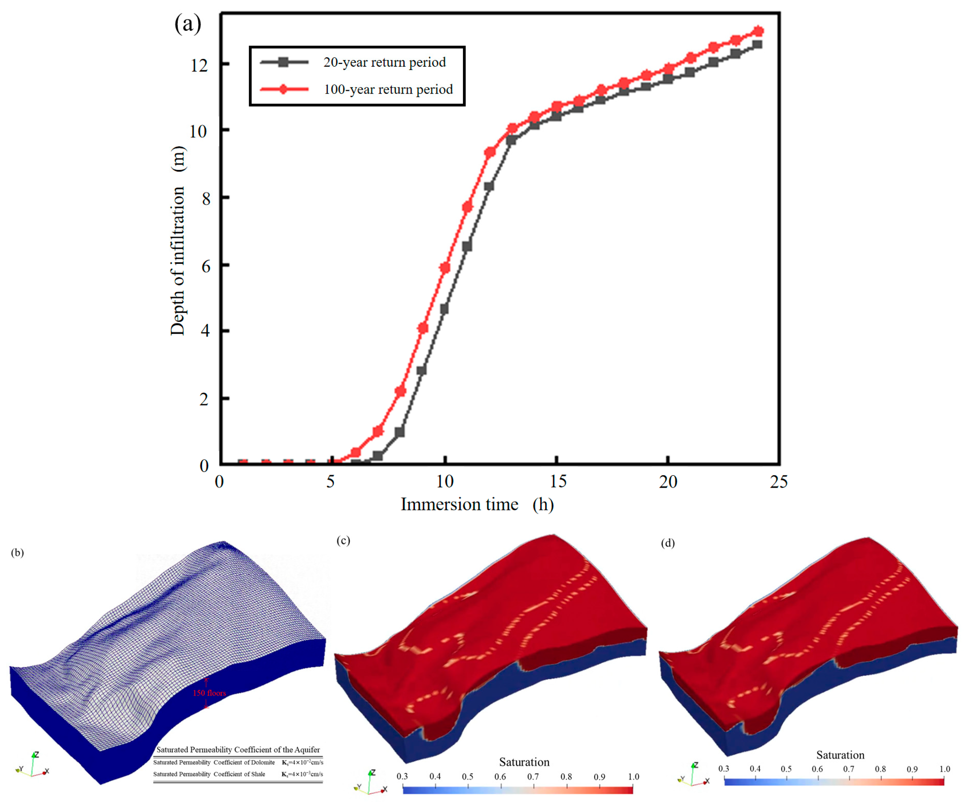
Based on the topological model of the surface, a rainfall calculation model was generated (Figure 15). In the X and Y directions, grids are divided with a spacing of 5 m and, in the Z direction, a grid spacing of 0.5 m is used to generate 110 layers of grids. The boundary conditions for the hydrological model are Dirichlet fixed-head no-flow boundary conditions.

The upper part of the landslide mass consists primarily of dolomite and shale, with well-developed joints and fractures. The rock is highly fractured, and the surface is intensely weathered, making it highly permeable with a large permeability coefficient. The saturated permeability coefficient for dolomite is set to Ks = 4 × 10⁻² cm/s and, for shale, Ks = 4 × 10⁻³ cm/s. The unsaturated rock and soil in this region are modeled using the van Genuchten model.

Under the 20-year return period rainfall conditions, it is assumed that all the rainwater infiltrates into the slope, without forming surface runoff. Under the 100-year return period rainfall conditions, some of the rainwater infiltrates into the slope while the rest forms surface runoff. Figure 15 shows the development curves of infiltration depth over time and the 3D model of infiltration saturation distribution. Initially, the soil is relatively dry and rainwater quickly infiltrates into the interior with a rapid infiltration rate. As infiltration progresses, once the shallow soil reaches a nearly saturated state, the rate of development of the infiltration peak stabilizes and proceeds inward at a constant speed. After 24 h of rainfall, the final infiltration depths for the two conditions are 12.5 m and 13.0 m, respectively. Since the permeability coefficient of shale is smaller than that of dolomite, shale has a certain water-blocking effect, resulting in a smaller infiltration depth in areas where shale is exposed compared to areas where dolomite is exposed.

To explore the stability of the landslide under rainfall conditions, the hydrological results from the previous section, including saturation, water head, and other information, were mapped onto the blocks within the current grid through grid interpolation. The corresponding blocks experienced increases in unit weight, body force, and strength reduction. For the 100-year return period scenario, the impact of surface runoff erosion on the upper surface units of the slope also needs to be considered. Based on the above hydrological information, a stability analysis of the landslide under rainfall conditions was conducted.

Figure 16 shows the variation of the displacement and crack number of key blocks with increasing Rf under different rainfall conditions. Under the 20-year return period rainfall probability, the curve shows a turning point at 1.06, at which the slope becomes unstable. After this point, displacement and crack number rapidly increase so the stability factor of the slope under the 20-year return period is defined as 1.06. Under the 100-year return period rainfall probability, the curve exhibits a sudden change at 1.04, where the cracks in the slope have already become through-going and the slope has entered an unstable failure state. Therefore, the stability factor of the slope under the 100-year return period is defined as 1.04.

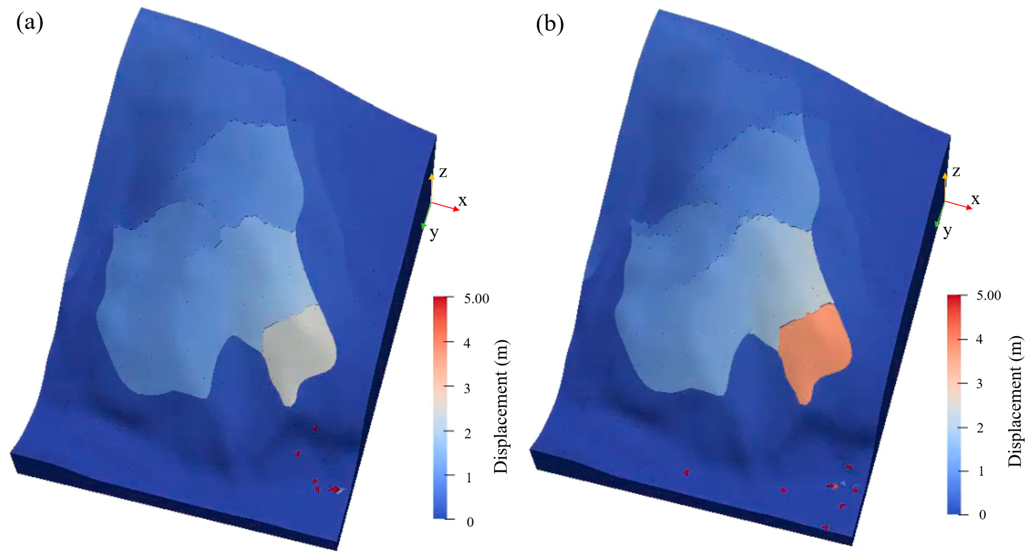
Figure 17 shows the deformation and failure process of the landslide mass under different rainfall probabilities. The calculations reveal that under rainfall conditions, the uppermost dolomite of the landslide is more affected, with displacements generally larger than in the natural state. Rainwater infiltrates along the fractures in the rock, softening the fracture structure, while infiltration pressure is generated within the fractures, increasing the gravity acting on the slope, reducing the cohesion, and intensifying rock deformation and failure. Under the 20-year return period rainfall conditions, cracks develop in the middle of the landslide, with larger displacements at the middle and front edges, pulling the rear slope and creating tensile cracks. Shear failure occurs on both sides of the slope. Under the 100-year return period rainfall conditions, landslide deformation intensifies, with continuous cracks in the middle, an increase in tensile cracks at the rear, and a downward sliding trend at the front edge, making the slope more prone to instability. Rainfall mainly affects the upper dolomite and shale layers, causing deformation at the surface, while the overall slope remains in a stable state.

5. Conclusions

This study utilized a combination of drone aerial photogrammetry, field geological surveys, drilling, geophysical exploration, trenching, and geotechnical tests to identify the spatial development characteristics and material composition of the Huangyukou landslide. A 3D model of the landslide was developed based on drone imagery and detailed measurement data used to analyze its deformation and failure characteristics, main triggering factors, mechanisms, development trends, and potential disaster scope. Ground-penetrating radar and high-density electrical methods were employed to determine the burial depth and coverage area of the Quaternary cover layer and fully weathered layer at the site.

A rainfall model for the Beijing area was developed in this study to analyze changes in the bulk density and shear strength of the rock–soil mass during the rainfall–runoff–infiltration process. This study also examined variations in pore water pressure and dynamic water pressure. Based on this, the infiltration saturation changes in the Huangyukou landslide under different rainfall intensity conditions were simulated, revealing the development pattern of the infiltration peak and final infiltration depth. Hydrological results from the simulation, including saturation and water head data, were mapped onto the model grid using grid interpolation. This allowed for the determination of corresponding changes in bulk density, body force, and strength reduction for each block, providing critical dynamic hydrological conditions and physical mechanisms for stability analysis.

Using field geological surveys, geotechnical tests, and drone-derived data, CoSim software (version 2024R11) was applied to assess the stability of the Huangyukou landslide under natural conditions and different precipitation scenarios (P = 5%, P = 2%, P = 1%). The integration of 2D and 3D numerical models verified the applicability of the rainfall–runoff–seepage coupling model in landslide stability analysis. The findings offer valuable theoretical support and practical guidance for regional landslide risk management and disaster prevention in the context of future extreme climatic conditions.

Under rainfall conditions, the landslide mass undergoes deformation and failure processes, such as crack propagation, pore water pressure accumulation, and the formation of a continuous sliding surface. Model simulations demonstrate that under extreme rainfall conditions, the shallow rock–soil mass first experiences localized instability, eventually forming a continuous sliding surface that leads to overall landslide failure. Strength reduction analysis revealed that the safety factors for the Huangyukou landslide under 20-year and 100-year return period rainfall conditions were 1.06 and 1.04, respectively. This study indicates that extreme rainfall exacerbates the deformation and instability risks of the landslide and rainfall intensity is significantly correlated with landslide stability.

The limitations of this study, including the reliance on a specific rainfall model, assumptions of uniform soil properties and simplified groundwater flow conditions, and the lack of long-term monitoring data, suggest directions for future research. Future studies could incorporate alternative rainfall models, more complex soil and groundwater flow conditions, and long-term monitoring data to improve prediction accuracy and capture seasonal or long-term variations in rainfall and landslide behavior.