An Interval Autocorrelation Mix-Up of Data Augmentation Based on the Time Series Prediction for Wastewater Treatment Model

Abstract

The abuse of chemical agents in wastewater treatment is very universal. However, accurate predictive models capable of addressing this issue rely on precise and abundant data. Limitations in sampling frequency and equipment often lead to insufficient data, resulting in model overfitting. To address this, the IA Mix-up data augmentation algorithm, based on correlation coefficient-weighted mixing, has been proposed. By ranking the temporal correlation of water quality data and incorporating error weight mixing into original labels, the algorithm adjusts mixed label weights according to the temporal characteristics of the original signal, preserving time-series correlation. Experimental results demonstrate an average 8.75% improvement in prediction accuracy across four neural network models, with R²-e reduced to 1–5%. Among the four prediction models, the LSTM model has the highest prediction accuracy of 89%. Compared with existing time-series data augmentation methods, IA Mix-up enhances the r value by 9.5%, improves prediction accuracy by 7%, and reduces the training-validation prediction error by 3.67%. These results indicate that the proposed algorithm effectively mitigates overfitting and enhances model performance. In actual use, the total phosphorus in the effluent meets the Class I effluent standards while saving 33% of polyaluminum chloride.

1. Introduction

The excessive use and waste of chemical agents in sewage treatment is very common. Therefore, it is crucial to accurately predict and control the use of agents. In recent years, artificial intelligence methods have been widely applied across wastewater treatment prediction. For instance, convolutional neural networks have been employed to forecast sludge aeration rates [1]. Researchers such as Wan explored water quality prediction using gated recurrent unit networks (GRUs) [2]. Concurrently, studies have demonstrated that increasing the volume of training samples for deep learning models can significantly enhance their accuracy [3]. However, practical engineering often faces challenges such as difficult data collection and insufficient data volume, leading to prevalent issues of model overfitting [4,5,6]. Notably, the implementation of deep learning models necessitates a significant quantity of data, which presents difficulties for municipal wastewater treatment plants (WWTPs) to achieve extensive operational automation [7]. To address this challenge, data augmentation has emerged as a direct and effective solution [8,9]. Recent studies have explored the application of data augmentation techniques to improve water quality prediction models. For instance, researchers [10] utilized the synthetic minority over-sampling technique (SMOTE) to address class imbalance in water quality datasets, achieving notable improvements in the recall rates of classification predictions using LightGBM and CatBoost models. Similarly, study [11] demonstrated that time-series data augmentation combined with the selection of lagged water quality features effectively enhanced the prediction of energy consumption in wastewater treatment plants, with the model’s MAPE reduced by 8.2% to 10% through the reinforcement of lagged energy consumption data to better capture temporal dependencies. In addition, researchers [12] applied data augmentation methods to compensate for insufficient observed rainfall data, confirming that predictive performance improved significantly after augmentation. Given that wastewater quality and dosing data inherently constitute continuous time-series data, with sampling intervals determined by the frequency of instrument measurements, small wastewater treatment plants—where data scarcity arises from sampling limitations—are selected as the focus of this study. This work specifically examines the effectiveness of time-series data augmentation techniques in enhancing the development of data-driven predictive models.

In the realm of time-series data augmentation, traditional methods such as cropping, flipping, adding noise [13], and frequency domain enhancement primarily consider the shape of individual sequences but are no longer suitable for enhancing high-dimensional sequence data [14]. Recently, methods based on original sequence decomposition and mixing have gained favor in preprocessing for deep learning models [15]. For instance, in a study predicting dam deformation [16], the original data were decomposed into trend, periodic, and disturbance components. The trend and disturbance components were predicted using deep learning models, demonstrating higher prediction accuracy compared with direct prediction. In another work, a borderline mix-up variant used a support vector machine (SVM) to select boundary samples, increasing the likelihood of boundary samples [17]. This mix-up data augmentation method was initially applied in image enhancement to regularize neural networks and reduce overfitting. Validation across six datasets showed that the mix-up method enhanced model generalization capabilities [18]. Another effective method involved mixing sequences obtained through the dynamic time warping (DTW) of original features [19]. Three types of dynamic time warping were compared with other data augmentation methods, resulting in an average improvement in prediction accuracy by 3–4%. Additionally, another study achieved dataset balance through a suitable sampling scheme and mitigated the negative impact of data duplication by generating synthetic time series using Fourier surrogates, improving overall accuracy from 90% to 96% [20]. Yan et al. proposed a method for variational mode decomposition (VMD) under the rolling method, which reduced RMSE by 16.69%, MAE by 13.02%, and MAPE by 11.90% when using a GRU network to predict NH3-N [21].

Furthermore, deep learning-based sequence augmentation methods applied to time-series data augmentation have shown promising results [22,23,24]. For instance, Yoon introduced generative adversarial networks (GANs) into time-series data augmentation [25]. They considered the differences between multidimensional and single time series and proposed TGAN networks to capture underlying relationships between different dimensional time series. Additionally, a fully connected layer-based auxiliary classifier generative adversarial network (FC-ACGAN) data augmentation method was employed to enhance spectral data, resulting in an average accuracy improvement of 5.13% compared with models using mix-up, which showed a 3.15% improvement [26].

In the WWTPs, where water quality and dosing data inherently consist of continuously changing time series [27,28], the sampling interval aligns with instrument measurement times, while chemical dosing remains fixed and excessive. Therefore, precisely controlling dosing has dual economic and ecological significance [29]. This paper proposes a new interval autocorrelation mix-up (IA Mix-up) method to solve the problem of overfitting in 2.3. The ability of the method to solve the overfitting problem is investigated by applying the prediction performance of the deep learning model in Section 3. Conducting experiments and validations on wastewater treatment datasets, the prediction accuracy of PAC agents has been improved by 7% compared with the traditional mix-up method. Considering that LSTM models often suffer from phase shift issues in time-series prediction, study [30] addresses phase shifts in multi-step time prediction by employing an updated LSTM network, and validates the approach in the frequency domain. In this study, the experimental section similarly applies FFT to analyze the spectral relationships of the predicted sequences. Due to the data-driven nature of deep learning models, overfitting issues often arise when these models are applied to various processes and parameters with insufficient dataset sizes to support effective predictions, especially in the field of wastewater treatment. The studies mentioned above demonstrate that data augmentation methods can effectively mitigate these challenges.

2. Materials and Methods

2.1. Long Short-Term Memory Algorithm

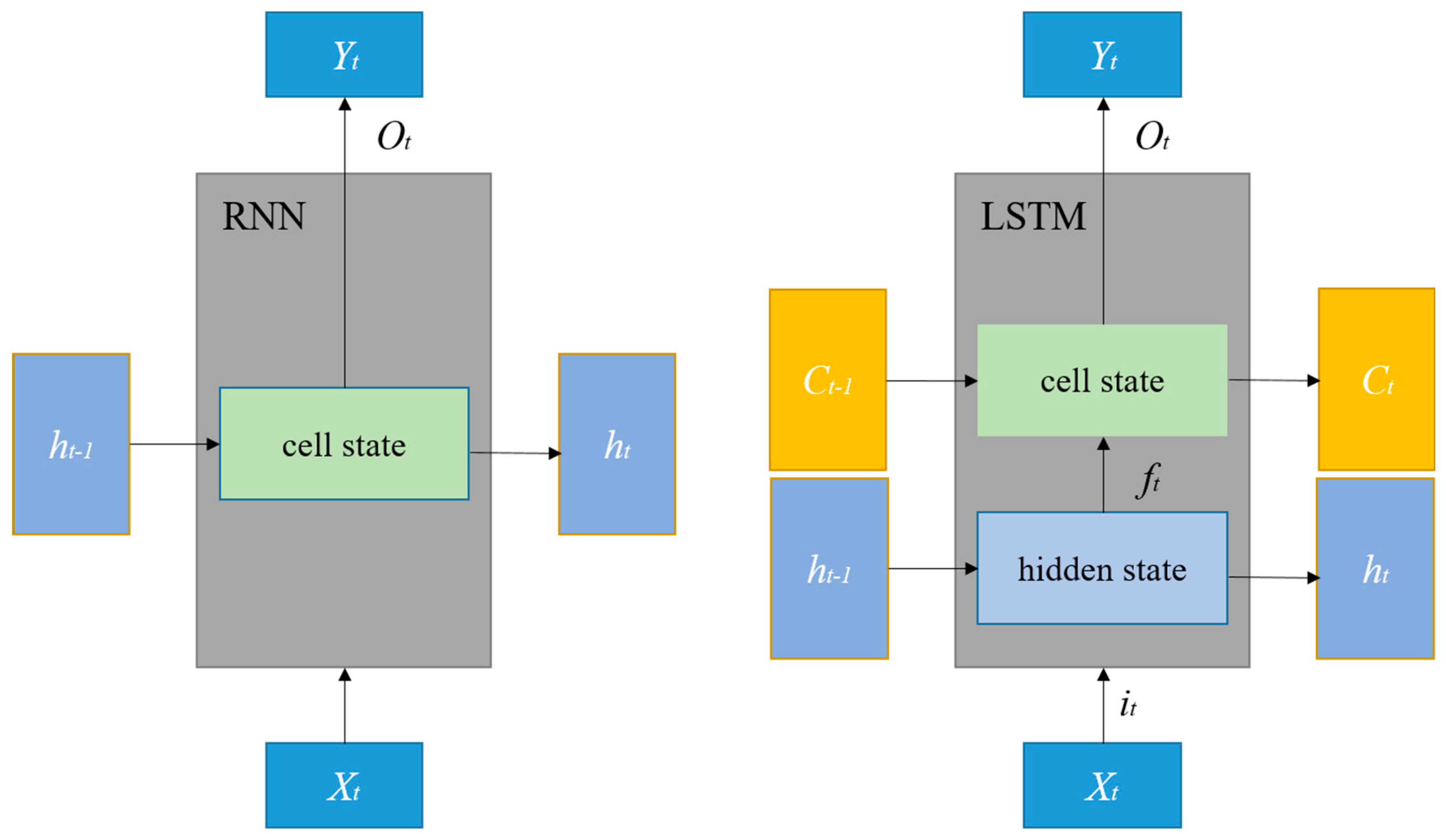
Recurrent neural networks (RNNs) belong to a category of recursive neural networks designed for sequence data input. Due to their sensitivity to temporal changes, RNNs have found applications in natural language processing and time-series data analysis [31]. The core idea of an RNN involves sequentially inputting sequence data according to the order of arrangement (such as time sequence or language structure). The relationship between input data, hidden layers $h^{(t)}$, and outputs $O^{(t)}$ is depicted. The information from the previous time step is passed on in the hidden layer $h^{(t)}$, and the information is retained. $O^{(t)}$ represents the model output, and the loss function $L(t)$ can be calculated based on the true value $Y(t)$. The loss L accumulates as the sequence progresses. For time step t, the relationship between the algorithm’s input, hidden layer, and output is given by Equations (1)–(3):

$$h^{(\mathrm{t})}=\varphi (\mathrm{U}{\mathrm{x}}^{(\mathrm{t})}+W{h}^{(\mathrm{t}-1)}+b)$$

(1)

$$O^{(t)}=V{h}^{(t)}+c$$

(2)

$$\hat{y}=\sigma (O^{(t)})$$

(3)

where the function $\varphi (x)$ is the activation function, and, in this study, the Tanh function is chosen. The function $\sigma (x)$ is the sigmoid function, used for the output layer activation in prediction.

The LSTM (long short-term memory) algorithm is an improved version of the RNN algorithm. In contrast to RNNs, which have only one state h, LSTMs have two states: cell state and hidden state [32]. Figure 1 shows the difference between RNNs and LSTMs. The mathematical expression is as follows:

$$f^{(t)}=\sigma (W_f^{(t)}\cdot [h^{(t-1)},x^{(t)}]+b_f^{(t)})$$

(4)

$$\sigma (x)={\displaystyle \frac{1}{1+\exp (-x)}}$$

(5)

$$i^{(t)}=\sigma (W_i^{(t)}\cdot [h^{(t-1)},x^{(t)}]+b_i^{(t)})$$

(6)

$$C^{\prime (t)}=\tanh (W_C^{(t)}\cdot [h^{(t-1)},x^{(t)}]+b_C^{(t)})$$

(7)

$$C^{(t)}=f^{(t)}{C}^{(t-1)}+i^{(t)}{C}^{\prime (t)}$$

(8)

$$h^{(t)}=\sigma (W_h^{(t)}[h^{(t-1)},x^{(t)}]+b_h^{(t)})\times \tanh C^{(t)}$$

(9)

In Equations (4)–(9), $f^{(t)}$ and $i^{(t)}$ represent the outputs of the forget gate and the input gate. $C^{(t)}$ is the cell state at time t, and $h^{(t)}$ is the output of the LSTM unit at time t. The LSTM algorithm selectively filters and transmits information by combining the outputs of the forget and input gates, achieving the screening and transmission of information related to the input data and the hidden layer state.

2.2. Data Augmentation Method Based on Mix-Up

To address the unique two-dimensional characteristics of data, the mix-up method, commonly used in image classification, is applied to augment time-series data. The goal is to mitigate overfitting caused by small sample sizes through data augmentation. The mathematical expression for the mix-up method is as follows:

$$\begin{array}{c}\tilde{x}=\lambda x_i+\left(1-\lambda \right)x_j\\ \tilde{y}=\lambda y_i+\left(1-\lambda \right)y_j\end{array}$$

(10)

In Equation (10), $x_i$ and $x_j$ are two randomly selected samples from the sample dataset, $y_i$ and $y_j$ are their corresponding labels, and λ is a weight coefficient between (0, 1) following a Beta (α, α) distribution, where α is the interpolation strength parameter.

Considering that a single sample in the time-series dataset is a one-dimensional vector data with a length equal to the LSTM model prediction timestamp, and a multidimensional sample set is a two-dimensional array, consistent with image information dimensions, the mix-up method transforms the empirical Dirac distribution in the sample space into an empirical neighborhood distribution:

$$P_{\delta }(x,y)={\displaystyle \frac{{\displaystyle \sum _{i=1}^n\delta (x_i,y_i)}}{n}}$$

(11)

$$P_v(\tilde{x},\tilde{y})={\displaystyle \frac{{\displaystyle \sum _{i=1}^{n}v({\tilde{x}}_i,{\tilde{y}}_i|x_i,y_i)}}{n}}$$

(12)

In Equations (11) and (12), δ is the empirical Dirac distribution function, v is the neighborhood distribution function, n is the number of samples in the training set, $\widetilde{x_i}$, $\widetilde{y_i}$ represents the $x_i$ generated samples and the corresponding labels.

2.3. Improved Interval Autocorrelation Mix-Up

The dataset generated by the method described in Section 2.2 will be utilized in the training set of the deep learning model to minimize empirical neighborhood risk. However, the distribution of pixel information in images exhibits spatial correlations, and time-series data with temporal characteristics show a certain correlation along the time axis. This correlation is manifested in the inherent connection of same-dimensional vectors in the sample. The single mix-up method cannot exploit this information effectively. To extract information changes along the time axis, this paper proposed a combination of autocorrelation function (ACF) coefficient and mix-up, which is called interval autocorrelation mix-up (IA Mix-up). For IA Mix-up to obtain the autocorrelation coefficient vector $w=[w_1,w_2,\dots ,w_k,\dots ,w_T]$, where T is the time-series data step, determined jointly by the ACF coefficient confidence interval and the data slice required by the LSTM model. The ACF coefficient can be calculated by Equation (13):

$$w_k={\displaystyle \frac{{\displaystyle \sum _{t=1}^{T-k}(x_t-\overline{x})(x_{t+k}-\overline{x})}}{{\displaystyle \sum _{t=1}^T{(x_t-\overline{x})}^2}}}$$

(13)

The sliced x after processing is a T × n two-dimensional array, where n is the input feature dimension, so $W=[w_1^{\prime },w_2^{\prime },\dots ,w_n^{\prime }]$. For any time series, the critical value of the 95% confidence interval of ACF values not significantly different from 0 is $\pm 1.96/\sqrt{T-d}$. This critical value indicates that, if the ACF coefficient is less than this value at a 95% confidence level, it is considered statistically significant in terms of autocorrelation at the time interval on the x-axis.

The autocorrelation coefficient vector w reflects the factors influencing the variable at time t due to the variables at the previous T times. After scaling, w is multiplied by the time-series data. Due to the uneven lengths of lag sequences in the sliced sequence, the rolling multiplication method is adopted. The formula for solving a single time series is as follows:

$${\mathrm{x}}^{\prime }(t+k)={\displaystyle \sum _{i=0}^{k}w[T-i]\cdot x(t+i)}(k=0,1,\dots ,T-1)$$

(14)

The obtained $x^{\prime }(t+k)$ calculated by Equation (14) is then substituted into Equation (10), resulting in a T × n dimensional array Equation (15)

$$x_i=[x_{i_1}^{\prime }(t),x_{i_2}^{\prime }(t+1),\dots ,x_{i_n}^{\prime }(t+T)]$$

(15)

which is a generated multidimensional time series. Figure 2 illustrates the schematic diagram of this algorithm.

In the IA Mix-up, the time information of the sequence is assigned to the weight factor of the mixing, so that the mixing method can not only process the relative space information of the two-dimensional sample but can also extract the time information of the sample itself. The new sample generated has the fusion time characteristics of the two original samples, used for data augmentation in deep learning models.

2.4. Data Augmentation Based on DBA Method and Time-GAN Network

The DTW Barycenter averaging (DTWBA) algorithm is a time-series averaging method based on dynamic time warping (DTW) [33]. This work refers to the method proposed in reference [34] to compute the average sequence for generating new sample data, thereby extracting different features from the original sequences and blending them to form a set of global features in time-series data. This method synthesizes an average sequence from the original data and is used in this paper as a data augmentation technique to generate data with similar features to the original data.

A random subsequence $X_{\mathrm{i}}=[x_{i1},x_{i2},\dots ,x_{iT}]$ is first selected from the original time series $X=\{X_1,X_2,\dots ,X_N\}$ to serve as the initial average sequence ${\overline{X}}^{(0)}$. Dynamic time warping (DTW) is then employed to align each input sequence $X_{\mathrm{i}}$ with the current average sequence ${\overline{X}}^{(k)}$, yielding:

$$DTW(X_i,{\overline{X}}^{(k)})=\{(t_i,t_{\overline{X}})\}$$

(16)

Subsequently, a new average sequence ${\overline{X}}^{(k+1)}$ is obtained. The DTW distance between the updated average sequence and the input sequences is repeatedly calculated until the following condition is satisfied:

$$||{\overline{X}}^{(k+1)}-{\overline{X}}^{(k)}||<\epsilon$$

(17)

At that point, the average sequence is considered to have converged and can be used for data augmentation or as a representative sequence.

The Time-GAN network, first introduced in this paper, is used for generating time-series data. In addition to the unsupervised adversarial loss on real and synthetic sequences, we introduced a step-wise supervised loss using the original data as supervision. This allows the model to capture step-wise conditional distributions in the data, considering the temporal information when calculating the loss. Time-GAN has been applied in the field of data augmentation [35], and, in this study, the code from the cited literature is referenced to enhance the data using the dataset from a wastewater treatment plant.

The main structure of the Time-GAN model consists of two sub-models—a generator and a discriminator—which are responsible for generating data and distinguishing between real and generated data, respectively. Through adversarial training between the two models, an optimal generative model is obtained, capable of generating time-series data that closely resemble the original data. The generator includes two functions—embedding and recovery—which provide a mapping between the feature space and the latent space, allowing the adversarial network to learn the underlying temporal dynamics of the data through low-dimensional representations. The embedding function e can be expressed as:

$$\begin{array}{l}{h}_S=e_S(s)\\ h_t=e_X(h_S,h_{t-1},x_t)\end{array}$$

(18)

In this equation, $e_S$ represents the embedding network model for static features, while $e_X$ denotes the embedding network model for temporal features using an RNN. Similarly, for the recovery function, r: $H_S\times {\displaystyle {\prod }_t{H}_X}\to S\times {\displaystyle {\prod }_{t}X}$ restores static temporal features to the feature space. Let:

$$\begin{array}{l}\tilde{s}=r_S(h_s)\\ {\tilde{x}}_t=r_X(h_t)\end{array}$$

(19)

where $r_S$ and $r_X$ represent the recovery feedforward networks for static features and temporal features, respectively.

The generator does not directly generate the sequence output in the feature space; instead, it first outputs into the embedding space. A random vector is extracted from the vector space as input to generate $H_S$ and $H_X$. The generation function g then extracts latent information from both the static and temporal feature spaces, with g implemented by an RNN function:

$$\begin{array}{l}{\tilde{h}}_S=g_S(z_S)\\ {\tilde{h}}_t=g_X({\tilde{h}}_S,{\tilde{h}}_{t-1},z_t)\end{array}$$

(20)

where $g_S$ represents the generator network for static features, and $g_X$ denotes the RNN generator for temporal features. Ultimately, the discriminator function d receives the feature encodings for both static and temporal data and returns the discriminator results ${\tilde{y}}_S,{\tilde{y}}_{1:T}=d({\tilde{h}}_S,{\tilde{h}}_{1:T})$. The discriminator results include the real input $h_{*}$, the synthetic input ${\tilde{h}}_{*}$, the real classification $y_{*}$, and the synthetic classification ${\tilde{y}}_{*}$. The discriminator function d is implemented using a bidirectional RNN network in the feedforward output layer:

$$\begin{array}{l}{\tilde{y}}_S=d_S({\tilde{h}}_S)\\ {\tilde{y}}_t=d_X({\overleftarrow{u}}_t,{\overrightarrow{u}}_t)\end{array}$$

(21)

2.5. Analytical Method

The determination methods of the relevant water quality parameters in this study are presented in

Table 1. Determination of water quality parameters.

Parameters	Testing Instruments	Testing Methods	Reference Standard
TP	TP Online Water Quality Automatic Monitoring Instrument	Ammonium Molybdate Spectrophotometric Method	GB 11893-89 [36]
COD	CODCr Online Water Quality Automatic Monitoring Instrument	Dichromate Method	HJ 828-2017 [37]
Water Flow/PAC	Electromagnetic Flow Meter	Electromagnetic Induction	ISO 6817 [38]

.

3. Results and Discussion

3.1. Deep Learning Framework

In this work, the LSTM algorithm is used as the main framework for the model. The model consists of an input layer, three hidden layers (LSTM framework), and one fully connected output layer. The input layer includes a data slicing layer, noise addition (Gaussian noise with sigma = 0.1), and normalization processing layer. The hidden layers also include a dropout layer, with a random dropout rate of 20–30%, and the number of neurons ranges from 64 to 256. Due to the gradient vanishing problem in the LSTM layer, the ReLU function is chosen as the activation function. The Adam optimizer is used with a learning rate adjusted to 0.005 and decayed with iterations. The loss function is set as the root mean square error with an L2 regularization term. All the code is implemented in Python 3.9 and the TensorFlow-2.12.0 framework.

3.2. Performance Evaluation Metrics

To measure the predictive performance of the deep learning model, three commonly used regression evaluation metrics are employed in this study: mean absolute error (MAE), root mean square error (RMSE), and adjusted R-square.

Mean absolute error (MAE):

$$MAE={\displaystyle \frac{1}{m}}\left|y_i-\widetilde{y_i}\right|$$

(22)

MAE represents the magnitude of absolute errors between predicted and actual values.

Root mean square error (RMSE):

$$RMSE=\sqrt{{\displaystyle \frac{1}{m}}{\displaystyle \sum _{i=1}^m(y_i-\widetilde{y_i}{)}^2}}$$

(23)

RMSE reduces the magnitude of errors to a constant level through square root operation. A smaller RMSE indicates a better fitting model as it implies smaller errors.

Adjusted R-square:

$$R^2=1-{\displaystyle \frac{{\displaystyle \sum _{i=1}^m{(y_i-\widetilde{y_i})}^2}}{{\displaystyle \sum _{i=1}^m{(y_i-\stackrel{-}{y_i})}^2}}}$$

(24)

$$Adjusted\_R^2=1-{\displaystyle \frac{(1-R^2)(m-1)}{m-p-1}}$$

(25)

where ${\stackrel{-}{y}}_i$ is the mean of actual values, p is the sample dimension, and m is the number of samples. Adjusted R-square ranges from [−1, 1], with higher values indicating better model accuracy. It adjusts for the impact of sample quantity on R-square, preventing the influence of ineffective sample quantity on model performance.

The Pearson correlation coefficient r and the p-value are used to verify the correlation between sequences. The r value ranges between −1 and +1, with 0 indicating no correlation and −1 or +1 indicating a clear linear relationship. The calculation formula for r is as follows:

$$\mathrm{r}={\displaystyle \frac{{\displaystyle \sum _{i=0}^N(x_i-\overline{x})(y_i-\overline{y)}}}{\sqrt{{\displaystyle \sum _{i=0}^N{(x_i-\overline{x})}^2{(y_i-\overline{y})}^2}}}}$$

(26)

Assuming x and y are derived from independent normal distributions, the probability density function of r is:

$$f(r)={\displaystyle \frac{{(1-r^2)}^{(n/2-2)}}{B(1/2,n/2-1)}}$$

(27)

where n is the sample size and B is the beta function. Under the null hypothesis H0: R = 0, which states that there is no linear relationship between the two variables, the p-value is the integral of the probability density function of r. At a significance level of 5%, if p < 0.05, we reject the null hypothesis and accept the alternative hypothesis, indicating that there is a significant linear relationship between the two variables.

3.3. Data Collection, Set Splitting, and Slicing

Data, including influent chemical oxygen demand (COD), total phosphorus (TP), and the phosphorus removal agent polymerized aluminum chloride (PAC), were collected. The sampling data collection point was at the high-efficiency sedimentation tank: TP, COD, and PAC dosages were collected at the entrance of the high-efficiency sedimentation tank; TP and water flow were collected at the outlet of the high-efficiency sedimentation tank. Experimental data from March 2023 to October 2023 were collected, totaling 150 samples. The experimental data used in this study were derived from the actual operational data of the Chengnan Wastewater Treatment Plant in Kangping County (42°31′ to 43°02′ N, 122°45′ to 123°37′ E), Shenyang, Liaoning Province, which has a treatment capacity of 10,000 cubic meters per day (with some facilities designed for 20,000 m³/d). In order to enhance the generalizability of the data, an additional 98 samples were collected from laboratories and other wastewater treatment plants with similar processes and treatment capacities.

In this study, real-time water quality data were collected using online water quality analyzers (Boxes, Yancheng, China). The chemical dosing data were obtained through a variable-frequency metering diaphragm pump equipped with online control capabilities (Qiaoruo, Suzhou, China). Both types of real-time data were transmitted via a wireless data transmission module to the central control unit for recording and storage. For the prediction of the phosphorus removal agent PAC, a total of 250 datasets were used. As the data volume was slightly small, 75% of the data were selected as the training dataset, 15% as the validation dataset, and 10% as the test dataset, randomly sampled from the overall data. Due to the use of the LSTM algorithm for multi-step prediction, the dataset needed to be sliced. Based on the calculated ACF coefficients and the wastewater treatment process, a time step of 7 sampling points was selected. This means that the water quality data for the first 21 h were used as input to predict the output indicators for the 24th hour.

3.4. Data Augmentation Experiments

3.4.1. IA Mix-Up Experiments and Analysis

The ACF coefficients for each time series of the phosphorus removal agent sample objectives were calculated and are presented in Table 1. The table displays the ACF coefficients at various lags for the sample data at a 95% confidence level.

Table 2. ACF coefficients of the samples.

Objectives *	t	t + 1	t + 2	t + 3	t + 4	t + 5	t + 6	t + 7	t + 8
COD	1	0.692	0.601	0.576	0.511	0.453	0.482	0.339	-
TP	1	0.882	0.787	0.735	0.695	0.621	0.506	-	-
TP-D	1	0.745	0.570	0.521	0.482	0.354	0.322	-	-
PAC	1	0.607	0.424	0.381	0.238	-	-	-	-

Notes: * COD represents the sedimentation tank inlet COD, TP represents the sedimentation tank outlet TP, TP-D represents the TP difference between the inlet and outlet of the sedimentation tank, PAC represents the PAC concentration (the PAC content present in each cubic decimeter of water, with the unit in milligrams).

shows that the COD at the inlet of the settling tank was most influenced by itself, with a seven-order lag coefficient, while the other parameters had lags of six and below. Given the sampling interval was set to three hours, the calculated T = 7 theoretically indicates that the addition of the phosphorus removal agent was influenced by the water quality changes in the previous 21 h. In practice, the addition of the phosphorus removal agent was affected by the influent water quality, and the stagnation time of water flow in the biochemical reaction tank was about 22.5 h, which corresponded to the calculated ACF lag coefficient T = 7. Therefore, considering all factors, T = 7 was chosen as the time step for the time-series data. Figure 3 illustrates the comparison of the water quality data enhanced by the IA Mix-up algorithm with the original sequence.

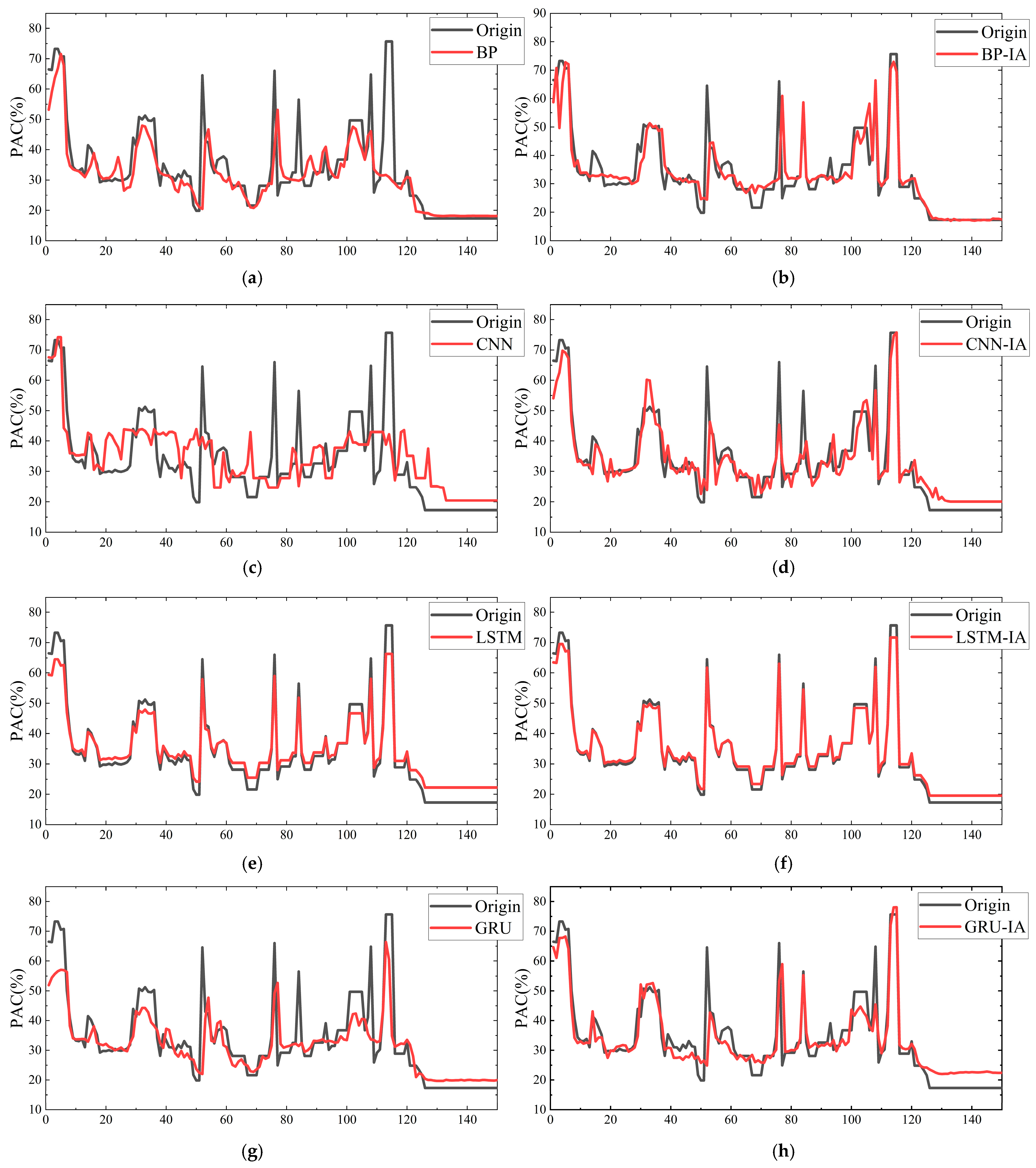
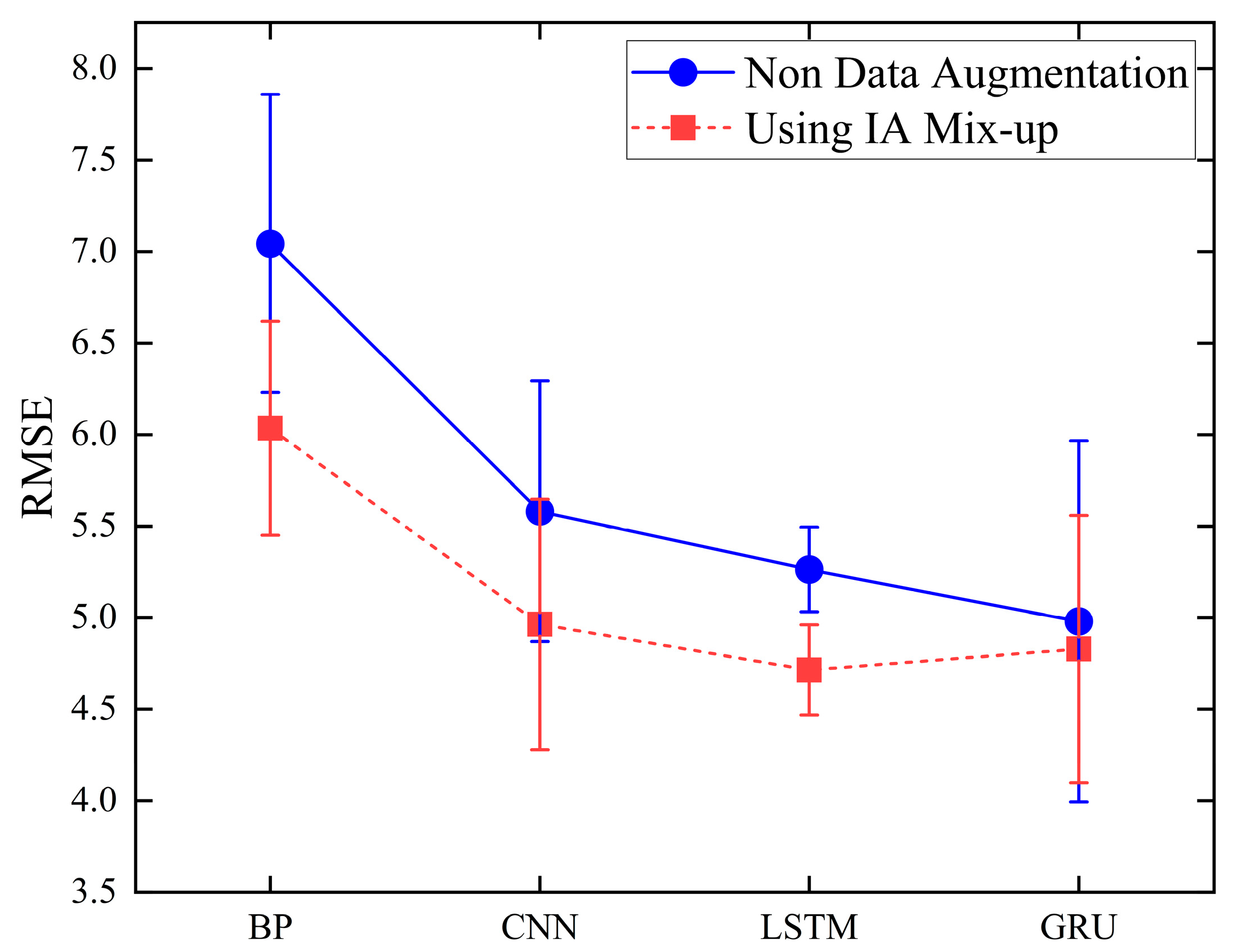
To visually test whether the IA Mix-up algorithm could address the issue of insufficient sample data and assess its robustness, Figure 4 was plotted. The figure includes the prediction curves of several neural network models before and after data augmentation using the IA Mix-up algorithm. In order to assess the robustness of the prediction model, the experiment corresponding to Figure 4 was repeated 50 times under identical conditions. The overall RMSE from each run was recorded, and the resulting mean and standard deviation were visualized as a point-line chart with error bars, as shown in Figure 5.

Analysis of the results before and after data augmentation with the IA Mix-up algorithm shows that, due to the insufficient number of samples for phosphorus removal agent prediction compared with the data requirements of the deep learning model, the lack of sample quantity led to an overfitting issue, resulting in the poor generalization ability of the model. After augmentation, the prediction errors of the four models generally decreased, and the prediction accuracy increased by an average of 8.75%. The data indicate that this algorithm effectively addresses the issue of insufficient water quality data, improving the prediction accuracy of water quality models. It is applicable to most data-driven artificial intelligence models and, due to its computational simplicity, can be widely used to expand the historical databases of most urban wastewater treatment plants.

From the perspective of prediction models, the CNN model is most influenced by the IA Mix-up algorithm. The LSTM model shows the best performance in PAC concentration prediction. Theoretically, this is because the CNN network model cannot maintain the advantages of a high receptive field when data are scarce, while the gate structure of the LSTM model effectively extracts hidden information from water quality data. Compared with the GRU network structure, which also performs well in wastewater treatment applications, the LSTM model, although slightly slower in computation, achieves improved prediction accuracy. Therefore, in the subsequent sections, this article focuses on further research of the IA Mix-up algorithm with the LSTM network structure in comparison with other similar data augmentation algorithms.

3.4.2. Comparative Experiments and Analysis on Correlation

The IA Mix-up presented in this paper, along with the traditional mix-up, DBA, and Time-GAN, was used to enhance the phosphorus removal data (PAC). Median filtering could be applied to the sequence for noise reduction to observe trends. Figure 6 displays the water data trend changes of the filtered sequence.

Figure 6 shows a comparison between the IA Mix-up augmented sequence and other algorithms. Overall, the IA Mix-up algorithm’s median filter curve for the four water quality datasets followed the same trend as the original sequence, indicating that the algorithm can effectively extract useful information from the time series. Additionally, compared with the other three augmented sequences, it demonstrated a faster response time and the smallest error. This means that the IA Mix-up method was more relevant. In order to reflect the correlation between sequences more intuitively, the Pearson correlation coefficient was introduced in this paper. The data augmentation experiments for the four types of water quality data were repeated 50 times, resulting in different generated signals. The Pearson correlation coefficient r was calculated for each set based on sequence similarity, and the mean and standard deviation of the r values were plotted as an interval chart, as shown in Figure 7.

Table 3. Comparison of r-values of sewage data.

Objectives	Mix-Up	IA Mix-Up	DBA	Time-GAN
COD	0.49	0.60	0.51	0.52
TP	0.53	0.49	0.37	0.46
TP_D	0.60	0.78	0.59	0.68
PAC	0.49	0.83	0.63	0.75

displays the mean Pearson coefficient r.

Table 4. Comparison of p-values of sewage data.

Objectives	Mix-Up	IA Mix-Up	DBA	Time-GAN
COD	1.7 × 10−7	4.9 × 10−11	5.7 × 10−8	2.2 × 10−8
TP	1.3 × 10−8	2.3 × 10−7	5.7 × 10−2	1.3 × 10−6
TP_D	7.2 × 10−11	3.7 × 10−17	1.0 × 10−10	6.2 × 10−15
PAC	1.8 × 10−7	1.6 × 10−19	2.9 × 10−12	3.1 × 10−19

displays p-values. The table contains r and p for the four types of water quality objectives under mix-up, IA Mix-up, DBA, and Time-GAN.

As shown in Table 3, the IA Mix-up method had the highest r-value, indicating the highest correlation—11% higher than mix-up and 8% higher than Time-GAN. The r-value for the other three methods differed by only within 3%. In Table 4, the Pearson (p) for the sequences generated by the four methods were all less than 10⁻², indicating a significant correlation between the generated sequences and the original sequences. Therefore, the data augmentation method proposed in this paper generates sequences that have the highest similarity to the original sequences, thereby retaining the information of the original sequences.

3.4.3. Comparative Experiments and Analysis on Dosing Prediction Models

Based on the experimental results in Section 3.4.1, the best-performing LSTM model for dosage prediction was selected. Data augmentation was performed using the mix-up, IA Mix-up, DBA algorithm, and Time-GAN network, and was compared with the baseline LSTM model without augmentation. Additionally, learning models used in the literature for water treatment were incorporated, and the prediction performance was evaluated on both the training and testing sets.

Table 5. Evaluation indexes of prediction models under each method.

Method	MAE	RMSE	R2	MAE	RMSE	R2
	Train *	Train	Train	Validation	Validation	Validation
LSTM	2.53	3.38	0.85	3.67	5.55	0.75
Mix-up	1.47	1.84	0.92	2.03	2.34	0.87
IA Mix-up	1.21	2.07	0.95	1.58	1.92	0.94
DBA	2.33	3.68	0.86	2.95	5.28	0.84
Time-GAN	0.90	1.18	0.97	2.13	2.34	0.93
Inter-BiLSTM	1.06	1.29	0.97	1.17	1.94	0.93
LightGBM	0.94	2.12	0.90	1.22	2.45	0.90

Note: * Train represents the training dataset; validation represents the validation dataset.

records and presents the results.

From Table 5, it can be concluded that when the deep learning model was trained on the original dataset, there was nearly a 10% discrepancy in the adjusted R² between the training and validation sets, indicating an overfitting issue. After data augmentation, the model’s MAE and RMSE decreased by 39% and 40%, respectively, and the error between the prediction accuracy on the training set and the validation set (R² error) was reduced to 1–5%, alleviating the overfitting problem. Compared with the mix-up method, the interval autocorrelation mix-up (IA Mix-up) method increased the validation set adjusted R² to 94%, improved prediction accuracy by 7%, and reduced the R² error to 1%, effectively addressing the overfitting issue. The Time-GAN network and the Inter-BiLSTM model achieved the best accuracy on the training set, with the trained models reaching a prediction accuracy of 97%. However, the R² error was 3% higher than that of IA Mix-up. In terms of MAE and RMSE errors on the validation set, both the Inter-BiLSTM model and the LightGBM model performed impressively, while IA Mix-up showed a slight advantage in accuracy. Additionally, the DBA algorithm exhibited underfitting issues, with an accuracy of 84%.

In summary, the proposed IA Mix-up method improved the model’s prediction accuracy on small sample datasets, with R² error outperforming the other three data augmentation methods. Furthermore, we assigned prediction tasks to the optimal models under five different conditions on the same test set. To evaluate the practicality of the model, it required 10% of the overall sample data as a test dataset for comparison. Therefore, the time consumed for a single test was at least two days. Figure 8 shows the comparison of PAC concentration prediction curves for each method.

As can be seen from Figure 8, the IA Mix-up method had the best fitting effect, whether it was a sharp place or a gentle place. The prediction accuracy of direct prediction and the traditional mix-up method was relatively poor.

Table 6. Evaluation indexes of prediction models on the test dataset.

Method	MAE	RMSE	Adjusted R2
LSTM	1.66	1.88	0.87
Mix-up	0.98	1.27	0.94
IA Mix-up	0.52	0.70	0.98
DBA	1.31	1.52	0.90
Time-GAN	0.82	1.07	0.96
Inter-BiLSTM	0.50	0.93	0.96
LightGBM	0.39	1.64	0.92

provides an intuitive comparison of performance metrics.

Table 6 demonstrates that the predictive model’s error and accuracy were significantly improved after data augmentation compared with the model without data augmentation. The proposed interval autocorrelation mix-up method could better extract time-series features from small sample datasets, expanding the original dataset. The MAE and RMSE of the model were reduced by 60% and 53%, respectively, while the accuracy increased from 0.87 to 0.98 (11.2%). The performance of Time-GAN networks was second only to the IA Mix-up method. Considering that the dataset used in this study did not meet the standard for training deep learning models due to its limited size, and that GAN networks required substantial data for learning and training, the time-series data generated by the IA Mix-up method were easier to calculate and more accurate to predict. Additionally, the Inter-BiLSTM and LightGBM learning models also demonstrated certain advantages, with both their MAE and RMSE being lower than those of the LSTM model optimized by the IA Mix-up algorithm. However, their accuracy was slightly inferior.

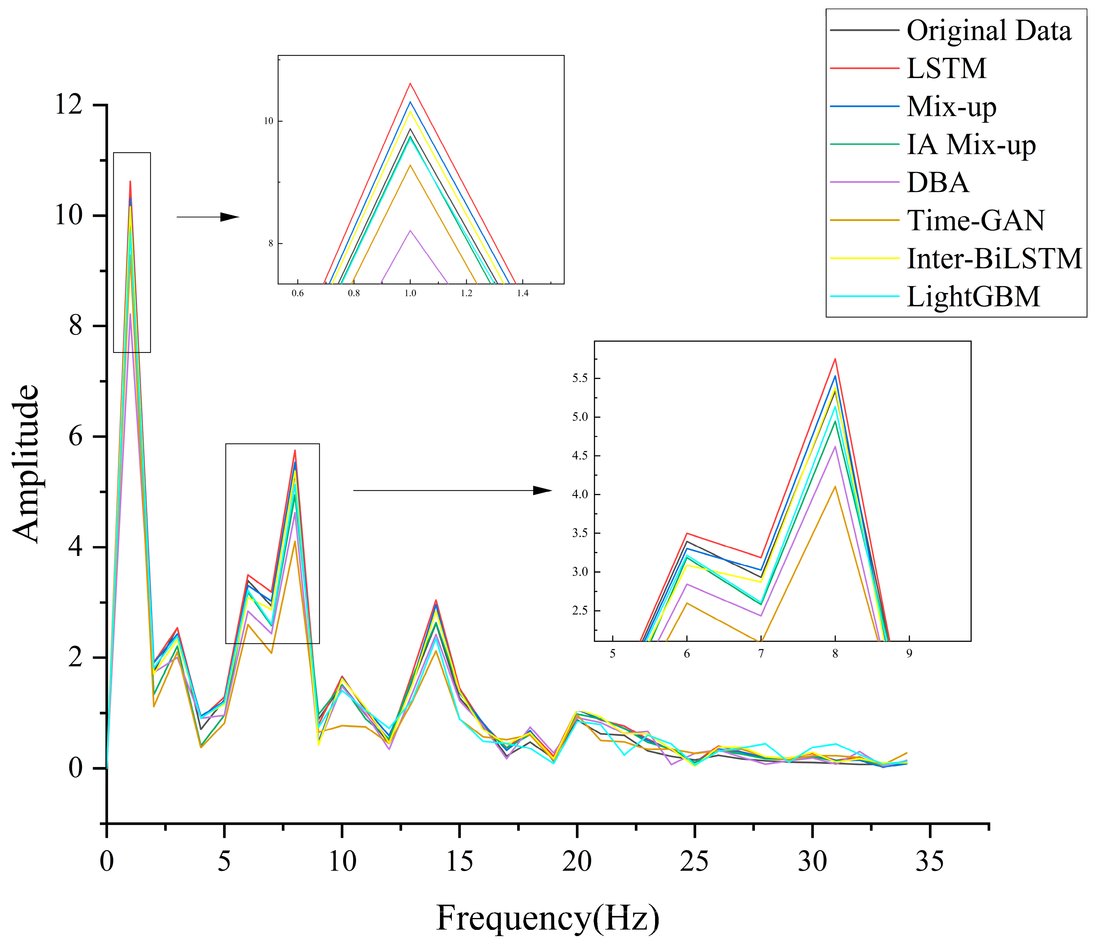
To analyze the spectral characteristics of the predicted time series in comparison with the original water quality data, we performed Fourier transform on the prediction results of the models shown in Figure 8 and presented the corresponding spectral comparison in Figure 9.

Figure 9 illustrates the frequency analysis, which shows that, when using the LSTM model for prediction, the common issue of phase lag between the predicted results and actual values did not occur. This was likely because the original water quality data lacked strong real-time responsiveness and clear periodicity, resulting in no phase shift in the single-step LSTM predictions.

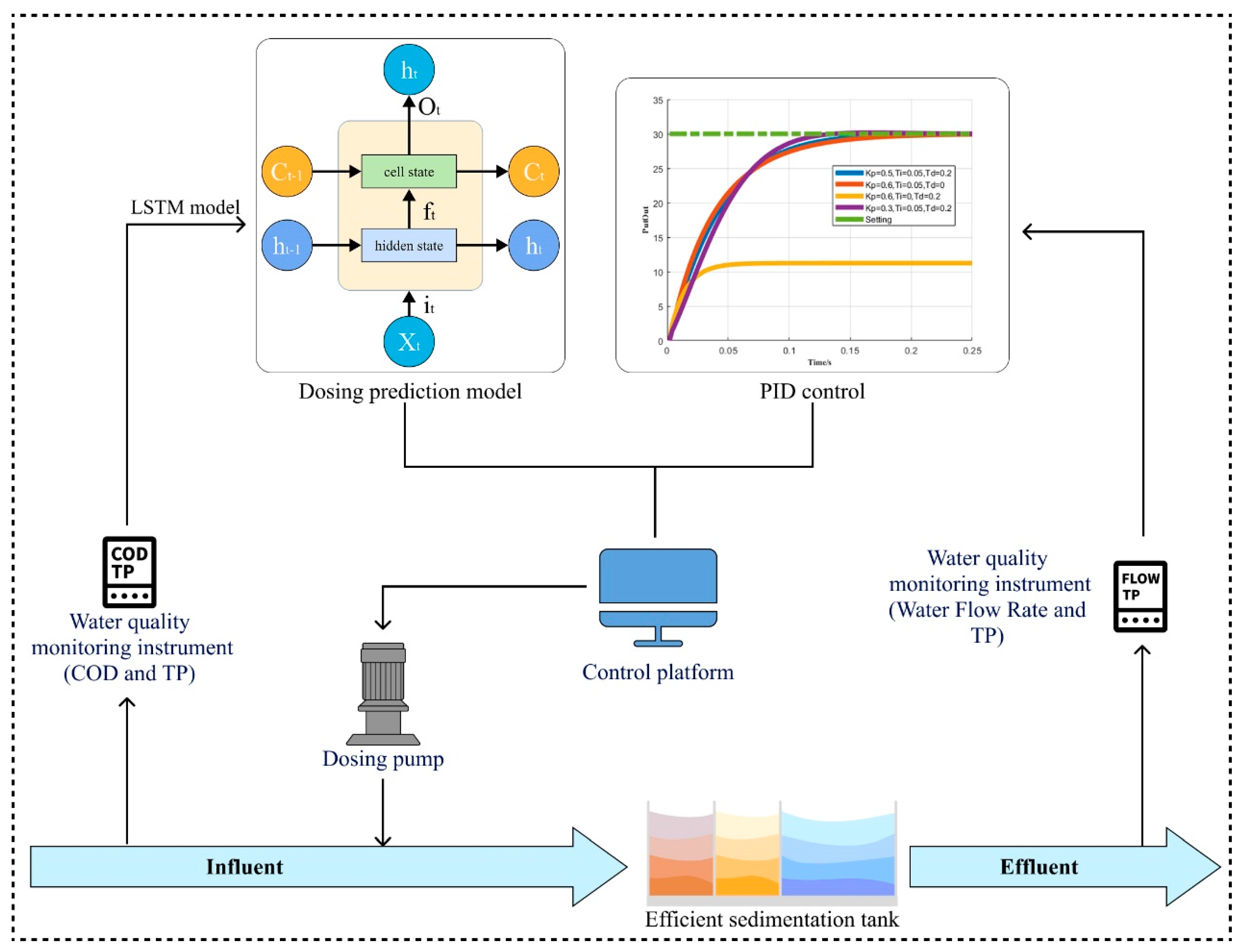
3.5. Validation of the Dosing Prediction Model in Municipal WWTP

The dosage prediction model trained using the algorithm proposed in this paper was coordinated with the automated dosage control program deployed at the inlet and outlet of the settling tank in the city’s wastewater treatment plant. The optimized PAC dosage strategy is implemented by controlling the digital dosing pump. The setting of the target value, combined with PID control, helps avoid unexpected predictions in certain extreme situations, improving the overall stability and reliability of the dosing model. The control processes are shown in Figure 10.

It is worth noting that the PAC dosing system has been operational in the wastewater treatment plant for nearly two months. Compared with the same period last year, the total phosphorus in the effluent meets the Class I effluent standards while saving 33% of polyaluminum chloride.

4. Conclusions

This study aims to address the challenge of building accurate reagent dosage prediction models for small-scale wastewater treatment plants where data scarcity limits model performance. To this end, we propose a novel data augmentation algorithm, IA Mix-up, which integrates autocorrelation function (ACF) coefficients into the traditional mix-up strategy through convolutional weighting.

Experimental results demonstrate that IA Mix-up significantly enhances data quality and model performance. Specifically, it improves the correlation coefficients of three key water quality indicators—COD, TP, and TP difference—by 15.5%, 11.6%, and 20.0%, respectively, compared with existing methods such as mix-up, DBA, and Time-GAN. It also reduces the prediction error between training and testing sets by 1–4%, and increases PAC dosage prediction accuracy by 2–8%. Across four different PAC prediction models, IA Mix-up achieves an average accuracy improvement of 8.75%, with the LSTM model showing the most pronounced gains—reducing RMSE by 39% and increasing accuracy by 14.5%. Moreover, the results in the frequency domain demonstrate that the dosing prediction model proposed in this study does not exhibit phase shift issues.

In practical deployment at a wastewater treatment plant in Shenyang, China, IA Mix-up facilitated precise PAC dosing, resulting in a 33% month-over-month reduction in reagent consumption. These findings highlight IA Mix-up’s strong potential for improving predictive performance in data-scarce environments, particularly in small to medium-sized wastewater treatment facilities facing equipment limitations.

Future work will focus on optimizing the input layer structure of the reagent prediction models to better extract correlations among water quality indicators and to compensate for time-lag effects, with the goal of further enhancing prediction accuracy and stability.