Dynamic Modeling of Coastal Compound Flooding Hazards Due to Tides, Extratropical Storms, Waves, and Sea-Level Rise: A Case Study in the Salish Sea, Washington (USA)

Abstract

The Puget Sound Coastal Storm Modeling System (PS-CoSMoS) is a tool designed to dynamically downscale future climate scenarios (i.e., projected changes in wind and pressure fields and temperature) to compute regional water levels, waves, and compound flooding over large geographic areas (100 s of kilometers) at high spatial resolutions (1 m) pertinent to coastal hazard assessments and planning. This research focuses on advancing robust and computationally efficient approaches to resolving the coastal compound flooding components for complex, estuary environments and their application to the Puget Sound region of Washington State (USA) and the greater Salish Sea. The modeling system provides coastal planners with projections of storm hazards and flood exposure for recurring flood events, spanning the annual to 1-percent annual chance of flooding, necessary to manage public safety and the prioritization and cost-efficient protection of critical infrastructure and valued ecosystems. The tool is applied and validated for Whatcom County, Washington, and includes a cross-shore profile model (XBeach) and overland flooding model (SFINCS) and is nested in a regional tide–surge model and wave model. Despite uncertainties in boundary conditions, hindcast simulations performed with the coupled model system accurately identified areas that were flooded during a recent storm in 2018. Flood hazards and risks are expected to increase exponentially as the sea level rises in the study area of 210 km of shoreline. With 1 m of sea-level rise, annual flood extents are projected to increase from 13 to 33 km² (5 and 13% of low-lying Whatcom County) and flood risk (defined in USD) is projected to increase fifteenfold (from 14 to USD 206 million). PS-CoSMoS, like its prior iteration in California (CoSMoS), provides valuable coastal hazard projections to help communities plan for the impacts of sea-level rise and storms.

1. Introduction

Coastal and inland flooding damages property and endangers lives. In 2021, natural disasters worldwide caused roughly USD 280 billion worth of damage, with USD 65 billion estimated to be caused by Hurricane Ida alone [1]. Many locations in the United States (U.S.) and around the world are experiencing increases in storminess and heavy precipitation events, a trend that is expected to accelerate with climate change and further exacerbate flood hazards globally (e.g., [2]). Coastal flooding is becoming more frequent and expensive as sea-level rise (SLR) accelerates [3]. Nuisance flooding is predicted to increase in the future [4], resulting in a doubling of flooding frequencies during the coming decades at many locations from the combination of SLR [5] and changes in storm and wave energy [6]. Additionally, and particularly for the Pacific Northwest, where precipitation already contributes to overland coastal flooding, rainfall intensity is expected to increase 20–50% by the 2080s [7].

Accurate assessments of flood hazards and risks are needed for awareness, prevention, and mitigation. Flood risk is defined here as the product of the probability of a flood event and the potential adverse consequences for human or economic activity (e.g., affected people or monetary value; [8]). Currently, several modeling systems exist that allow for physics-based modeling of flood hazards. The Sea-Level Rise and Coastal Flooding Impacts Viewer [9] estimates coastal flooding associated with climate-driven sea-level rise based on a static ‘modified bathtub’ approach, incorporating SLR and astronomical tides only. This method is practical and easy to implement but misses important local dynamics (e.g., wave-driven water levels and storm surges) of the flood event. The Federal Emergency Management Agency (FEMA) also provides nationally recognized flood hazard maps, called the Special Flood Hazard Area (SFHA). SFHA is defined as the area that could be flooded with a 1-percent chance of occurrence in any given year, also referred to as the base flood elevation or 100-year flood. SFHA is calculated from a set of hydraulic models that meet requirements for mapping. It does not provide information on more frequent events (e.g., the annual event) nor the effects of sea-level rise and/or projected climate change on flooding. Both NOAA and FEMA flood products are available across most of the U.S. The Coastal Storm Modeling System (CoSMoS; [10]) has generated detailed predictions of storm-induced flooding for California, incorporating coastal water levels driven by astronomic tides, surge, waves, sea-level anomalies, and riverine flows. However, it does not investigate all possible combinations of the land-based components of coastal compound flooding (i.e., a phenomenon in which two or more flooding sources occur simultaneously; [11]).

In this paper, we introduce, validate, and apply a workflow for the analysis and prediction of both frequent and infrequent compound flooding hazards and risk on spatial scales of hundreds of kilometers across different geomorphic settings and for dozens of realizations (i.e., events driven by tide, surge events, and wave-driven storms, but also several sea-level-rise scenarios). This is part of the Puget Sound Coastal Storm Modeling System (PS-CoSMoS), which has been designed to assess flood hazards ranging from nuisance flooding to severe storms for the current and future climate, incorporating SLR projections and changes in atmospheric forcing for fjordal estuary environments like the Salish Sea. This work improves upon model frameworks developed for San Francisco Bay [12], and other areas across California [13], demonstrating that PS-CoSMoS can be utilized across other sheltered estuaries throughout the world. This paper will focus on the overland flooding component of the workflow for a novel application in Whatcom County, Washington.

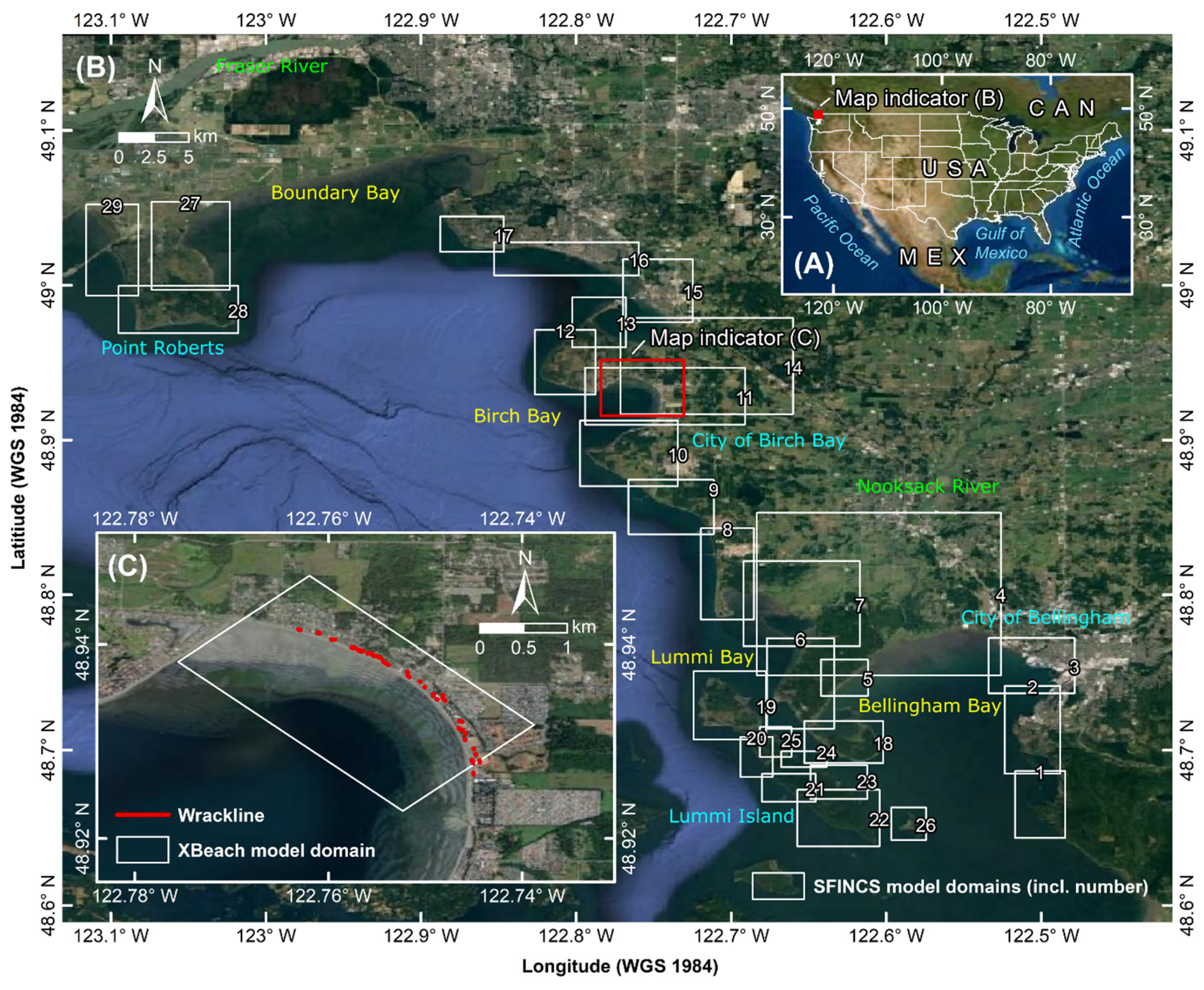
2. Study Site

The Salish Sea is a large fjordal system of flooded glacial valleys that includes the Strait of Georgia, Puget Sound, and the Strait of Juan de Fuca shared between British Columbia, Canada, and Washington State (Wash.), United States. This geomorphically diverse estuarine system is comprises a network of channels, shoals, and islands, encompassing numerous watersheds that provide fresh water to the region. The shoreline is highly meandering and complex and extends 2600 km just within the United States portion of the Salish Sea. Swell from the ocean propagates into the basin along a narrow portion of the Salish Sea through the Strait of Juan de Fuca, while local winds dominate the wave climate elsewhere.

Whatcom County is located in the northwestern corner of Washington, bordered by the Canadian Lower Mainland to the north and the Salish Sea to the west (Figure 1). It covers approximately 5460 km² and is home to diverse geology and ecosystems ranging from coastal estuaries to glaciated volcanic peaks. The total shoreline length is estimated to be 210 km. Whatcom County’s estimated population is ~228,000, with the largest population center being the coastal city of Bellingham with almost 100,000 housing units with a median value of USD 369,000 [14]. The largest contributors to GDP in Whatcom County include manufacturing, real estate, government, and health care. Accurate risk estimates are needed from shoreline planners that better address the magnitude and joint probability of the compound effects of sea-level rise and extreme events on people and property.

Elevations in Whatcom County range from sea level to a high point of >3000 m at the active volcano Mount Baker. In geological times past, the Fraser River in the Lower Mainland of British Columbia had a southern fork, creating the flat geography of a delta plain in that area that ensures productive farmland for dairies and berry growing called the Fraser Valley. The Nooksack River drains the area around Mount Baker, similar to the Fraser River, through the lower agricultural area and drains into Bellingham Bay. Other important areas in Whatcom County are (1) Lummi Bay with Lummi River, a historical distributary of the Nooksack River; (2) Lummi Island, just west of the coast of Bellingham; and (3) the United States–Canada border at the 49th parallel, which created Boundary Bay and the United States’ portion of Tsawwassen Peninsula called Points Roberts. Beaches are characterized by a platform that reaches between the mean lower low water (MLLW) to the base of the coastal bluffs. Extensive sections of the shoreline consist of engineering features in the form of sea dikes and armoring or low-lying delta between mean higher high water (MHHW). As a result of this characteristic morphology, minimal wave energy is dissipated at high tide, and waves impact the beach directly [15].

The tides in the Salish Sea are classified as a mixed semi-diurnal meso-tidal regime in which tidal ranges are amplified when propagating into the system from the Pacific Ocean, with a ~2 m tidal range in Bellingham Bay. Storm events are primarily driven by intense low-pressure weather systems originating in the eastern Pacific Ocean that make landfall between Oregon and Vancouver Island, British Columbia [16]. Coastal impacts and high-water levels in the Salish Sea are, therefore, influenced by a combination of offshore (Pacific Ocean) steric sea-level anomalies, inverse barometer effects, and local wind-driven setup. Maximum surge levels are generally in the range of 0.8 to 1.0 m (e.g., [17,18]). The wave climate in the Salish Sea is complex; swell dominates on the outer coast and western Strait of Juan de Fuca (wave periods typically >10 s), while wind-sea (wave periods typically <5 s) is dominant in the Georgia Straight and Puget Sound with wave heights generally less than 2 m [18].

3. Materials and Methods

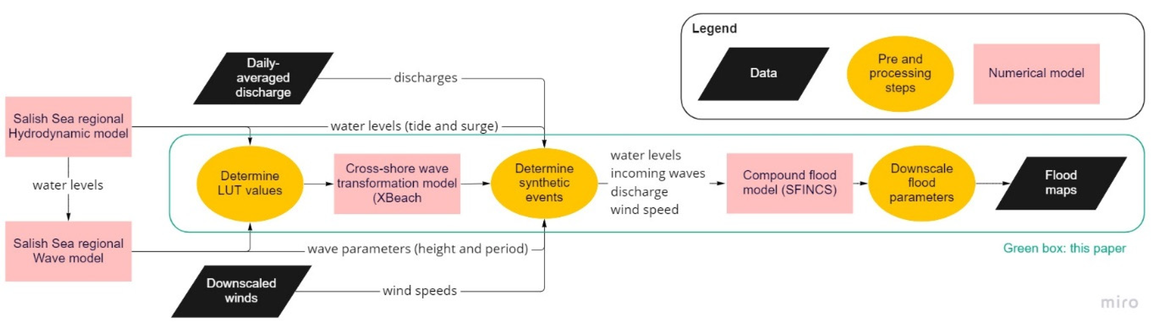
3.1. Overview

The framework utilizes multiple numerical models that interact to achieve the goal of predicting overland flooding (Figure 2). Two of the model components, (1) the regional hydrodynamic (tide-surge) model and (2) the regional wave model for swell and wind waves, are described in detail in separate manuscripts [19,20]. This manuscript focuses on overland flooding. The numerical methods applied for the computation of overland flooding are based on a series of cross-shore-profile model applications using XBeach [21,22] and overland flooding model domains using SFINCS [23]. These models were generated and automatically linked using MATLAB R2022a scripts that were developed to create, process input/output data, and run the models.

First, regional boundary conditions are based on (1) the hydrodynamic (tide–surge) model as developed by [19] and (2) the wave model for swell and wind waves developed by [20]. The regional hydrodynamic model is a Delft3D Flexible Mesh [24] model to compute tides and surges across the Salish Sea. The regional wave model is a combination of a linear transformation of Pacific Ocean swell and locally generated wind waves. Moreover, data on daily averaged discharges and downscaled winds are used as inputs to the entire workflow (details described below).

Secondly, the XBeach transect-based models were generated based on the local shoreline orientation and forced with a range of water levels and wave heights for the Whatcom County study domain in order to create a lookup table (LUT). This approach was followed to reduce the computational costs when computing static wave setup and dynamic incoming wave forcing close to the SFINCS boundary.

Thirdly, a series of two-dimensional SFINCS domains were generated along the same shoreline extent as the XBeach transects (see Figure 1B). SFINCS domains were run for hundreds of synthetic storms in order to determine compound flood hazards on a cell-by-cell basis for future climate conditions (sea-level rise and changes in fluvial, wave, and storm surge conditions). The domains were forced with water levels and waves generated from the XBeach-based LUT. Required input data and individual components are described below, followed by detailed explanations of the numerical methods.

3.2. Input Data

3.2.1. Topo-Bathymetry and Land Roughness

Prior to generating the XBeach and SFINCS models, elevation data were extracted along the entirety of coastal Whatcom County from the Coastal National Elevation Database (CoNED) topographic model of Puget Sound [25]. The CoNED dataset provided a seamless digital elevation model (DEM) at 1 m resolution and was constructed using the most recent, high-resolution datasets available (e.g., light detection and ranging (Lidar) topography, multibeam and single-beam bathymetry, etc.) merging them into a continuous surface. Here, the CoNED data were extracted between the −10 m isobath up to the +10 m elevation contour (referenced to NAVD88) to create the necessary DEMs for XBeach and SFINCS to account for all plausible scenarios of sea-level rise up to the year 2100. CONED elevation has a root-mean-square error (RMSE) of 22 cm. The subsampled CoNED DEMs characterize the morphology of the nearshore, beach face, and cliff surfaces as accurately as possible to enable robust predictions of the wave runup and hydrodynamic processes that influence flooding.

Data from the National Land Cover Database (CONUS; [26]) were converted to roughness values using Manning’s coefficients following [27] to define a spatially varying roughness value across each SFINCS model, while friction in open water is set to 0.020. As a result, land roughness varied between 0.020 (open water) and 0.15 (forest).

3.2.2. Meteorological Conditions, Water Levels, Waves, Discharges, and Sea-level Rise

The atmospheric forcing for PS-CoSMoS utilized hourly wind data predictions (10 m above the sea surface) from different sources. For the validation study, the historical nowcast of the Canadian High-Resolution Deterministic Product System (HRDPS) model was used, while the Geophysical Fluid Dynamics Laboratory (GFDL) CM3 model for CMIP5 (CMIP5-GFDL-CM3) [28] was used for the future climate runs. Atmospheric pressure was not included within the smaller SFINCS domains since variations are deemed negligibly small and were accounted for by the regional water level model [19] used to force the XBeach and SFINCS models.

PS-CoSMoS applies a Delft3D Flexible Mesh model to compute tides and surges across the Salish Sea. The model is highly skillful in reproducing still water levels (SWL) with a mean error of ~10 cm across 6 NOAA tide stations and seven additional USGS tide gages over the period 2017–2019 [29]. Still water levels, defined here as water levels driven by tide, steric sea-level anomalies, and storm surges were directly based on the regional Delft3D FM model and applied to describe time-varying water-level variations. For more information, one is referred to [19].

Waves were computed from the combination of local wind waves and linear transformation of swell accounting for the time-varying water level output from the tide-surge model. This approach allows for rapid wave predictions on high spatial resolution and long-term regional predictions and uses a similar skill compared to typical SWAN [30] implementations. Wave height and period are applied to compute wave transformation. For more information, one is referred to [20].

Daily averaged stream discharge forcings were prescribed at 23 locations throughout the Salish Sea. In particular, data from [31] for United States rivers were used. Data for the Fraser River are based on data from the Environment and Climate Change Canada Historical Hydrometric Data. For further information on discharges one is referred to [19]

In order to investigate the effects of sea-level rise (SLR) on coastal flooding in Whatcom County, eight SLR scenarios were assessed. In particular, 0, 0.25, 0.50, 1.00, 1.50, 2.00, 2,5. 3.00, and 5.00 m relative to the present epoch (1983–2001) are considered. In this paper, several sea-level-rise values were used instead of a specific time horizon in order to bracket the plausible magnitude of sea-level rise and enable reassessment of flood timing as refined relative sea-level-rise estimates are published by the scientific community. For example, Ref. [3] projected a relative sea level along CONUS of about 0.6–2.2 m in 2100 and 0.8–3.9 m in 2150. In this paper, downscaled sea-level values at Vancouver, British Columbia, for the five categories (low, intermediate–low, intermediate, intermediate–high, and high) from [3] are used to provide a time axis for modeled sea-level rise.

3.2.3. Exposure and Hazard Layers

Damage computations were performed with HydroMT-fiat (https://github.com/Deltares/hydromt_fiat, accessed on 27 May 2022; #19), which is a Python package developed by Deltares, the Netherlands. Delft FIAT (Flood-Impact Assessment Tool; v0.2.1) is a flexible open-source toolset for building and running flood-impact models that are based on the unit-loss method [32]. Inputs for FIAT are the hazard layer (flood extent and water depth with a certain probability of occurrence), exposure layer (object map with maximum USD damage), and vulnerability (depth–damage curves).

The exposure layer used in Delft-FIAT is based on a method that combines Global Urban Footprint (GUF; [33]) for the presence of buildings and Global Human Settlement Layer (GHSL; [34]) for population density. Subsequently, building value is estimated by combining GUF and GHS with characteristic values for population size and gross domestic product per capita, distributing these values equally across all buildings. The result is a method that can produce an exposure layer for any place on the globe. In this paper, we used a population size of 226,847 for Whatcom County based on the 2020 Census. Depth–damage curves and the relationship of construction cost per capita were based on [35]. Values were optimized to represent the local distribution between land cover types, including residential, commercial, and industrial. For the United States, a maximum damage per capita of USD 119,865 was used based on HydroMT-fiat but corrected for reported inflation between 2010 and 2020 (an 18.69% increase from USD 100,990) in order to reach the values reported in 2020. Human settlement is assumed to be static in time and thus does not develop nor respond to sea level. Moreover, all reported damages are represented in 2020 values.

3.3. Numerical Methods

3.3.1. Cross-Shore-Profile Model

XBeach [21,22] was applied in one dimension to estimate the cross-shore wave transformation and wave setup along each transect. XBeach was thus run in profile mode (as opposed to 2D mode) to reduce computational expense. The XBeach model was not calibrated but model skill was quantified (see below). The model was applied with standard parameters throughout this study. The 2-layer non-hydrostatic version of XBeach (XB-NH+; [36]) was used. Wave growth due to wind cannot be included in XB-NH+. A constant grid spacing of 0.5 m was used, which satisfies the numerical requirements of ~50 points per wavelength for a wave period of 4.5 s. The transect runs from deep water (~6 m) up to +10 m NAVD88 (maximum runup extent) for the most extreme conditions. For a wave period of 3.5 s, this equates to a kh value (i.e., wave number k multiplied with the water depth h) of less than 3 which is the required range for a 2-layer non-hydrostatic model. In the alongshore direction, every 50 m a transect was created. This resulted in 3409 transects for the entire Whatcom County.

An additional two-dimensional XBeach-NH+ model (XB-2D) was created to compare and verify the model results to observed flood extents (see Figure 1C). The XB-2D model was nested in the same regional hydrodynamic and wave model and compared to SFINCS maps (i.e., model–model comparison). Grid spacing for the 2D validation was set to 2 m in the alongshore direction and 0.5 m in the cross-shore direction. The alongshore distance is 2400 m, and the cross-shore distance 1400 m. The other settings are similar to the default of XBeach (and profile models).

3.3.2. Overland Flooding Model

SFINCS [23] was applied to predict overland flooding. SFINCS is a reduced-complexity model that approximates the shallow water equations similar to Delft3D and other physics-based models but with at least 100-times-lower computational expense. High-resolution topo-bathymetry and land roughness were included in the native 1 m resolution utilizing subgrid lookup tables [37]. The flux computations were performed at a 10 m resolution to reduce computational expense. This equates to ~10 points per wavelength for a wave period of 25 s. In total, 29 sub-domains across Whatcom County were generated using a semi-automated routine that optimizes domain size with less than 100,000 cells per domain. The SFINCS model was not calibrated but instead applied with default parameters throughout this study. Advection was activated and includes a small limiter (keyword advlim = 1) to reduce instabilities caused by large advection terms. The overland flood depth was subsequently downscaled from the maximum water levels on the flux grid to 1 m resolution using the nearest-neighbor interpolation in combination with a box filter of 3 cells.

Still water levels (tide and surge) and wave setup + incoming waves from the XBeach transects were imposed around the 2 m isobath which performed as the model boundary. Spatial variability in wave conditions from the transects was included. Wave energy for periods shorter than 25 s was excluded from the incoming signal since shallow water equation solvers (such as SFINCS) have an accurate dispersion relationship for kh < 0.1. This simplification results in an underestimation of the computed overland flooding. Moreover, the SFINCS model was also forced with a wind speed which resulted in a locally generated setup and discharges from local rivers and tributaries.

3.3.3. Computational Framework

Wave Transformation Lookup Tables

Transects for XB-NH+ were run as a lookup table (LUT) for 8 water levels between MSL and the highest computed water level and 5 wave heights between 0 and maximum computed wave height with constant steepness (total of 40 simulations). Values were selected based on the continuous time series from the large-scale hydrodynamic and wave models. Wave setup was extracted at 20 cm depth and linearly interpolated from the LUT. No wave-driven setup was imposed for inlets. However, an alongshore filter is applied to remove large alongshore gradients. Waves at the boundary of the XBeach transects were based on a spectral fit with a random signal based on the methodology of [38]. In particular, per transect, we filtered the incoming and outgoing waves and used the incoming surface level elevation to fit a Gaussian (for low-frequency energy) and JONSWAP (for high-frequency energy) spectra. Subsequently, the parameters of these fits for the events were simulated. A random signal per transect was computed. Each transect has its own variance-density function. However, the same random phase difference per frequency for all transects was used. Again, wave energy for periods shorter than 25 s were excluded.

Synthetic Record Generation

The downscaled GCM coupled with the regional hydrodynamic and wave model was used to describe the future climate. This climate is based on an 85-year time-series output of the GFDL-CM3 model for the period (2015–2100) simulating the RCP 8.5 emission scenario. In order to generate more realizations/events, 300 years of continuous synthetic records were generated based on water levels and wave parameters computed from the original 85-year forecast. The 300 years was chosen to determine a reliable 1–100-year event (1% chance event) with an empirical extreme value analysis, for which 85 years of data are not sufficient. This record length was chosen to have a sampling error less than ~5 cm in the return value estimate of SWL extremes with a return period of 100 years (99% confidence interval). The synthetic record was created by, first, decomposing the non-tidal residual (NTR) by subtracting a tide-only simulation (i.e., without meteorological forcing or steric sea-level anomalies) from the still water level. Second, the longer synthetic record was generated, assuming independence between the tides and NTR. In practice, this synthetic record generation means that a storm event could occur both during high and low tide. The synthetic record was constructed by randomly selecting a yearly NTR signal from the 85-year record. A uniform distribution shift from −1 to +1 days was applied to the time axis of the NTR to increase variability. Tides were generated from astronomical components computed from the tide-only regional-model results of [19]. Meteorological and wave conditions were assumed to be completely correlated with NTR and associated wind and wave conditions are directly used in model forcing.

Storm Selection

From the 300-year synthetic record, the largest storms were selected to run in the overland flooding model domains throughout Whatcom County. Particular storms (or events) were selected based on a total-water-level (TWL) proxy based on [39]. Total water level is defined here as the still water level in addition to wave-driven processes such as setup and swash. We applied a minimum storm duration of 3 days to find independent peaks. This storm selection was performed per transect, and the threshold is set to find the yearly maximum-water-level event (i.e., 300 events for 300 years of synthetic record). The unique storms were combined per SFINCS domain which resulted in 308 to 371 events per domain. Note that this is slightly more than 300, since not every transect has the exact same events. Each event was run for a daily tidal cycle around the peak. The simulation was initiated at low water of −0.5 m NAVD88 to avoid low-lying flooding areas in the backshore. In this iteration of the model framework, no extra events were included based on the discharge.

Extreme-Value Analysis

Flood hazards were determined on a cell-by-cell basis in the SFINCS model domains with an empirical frequency of exceedance and thus without fitting an extreme-value distribution (e.g., GEV or GPD). This approach allows for the full range of compound flooding options without having a priori knowledge of the combination of forcing conditions that lead to these events. The maximum computed water level, maximum velocity, and the time wet per event per grid cell were stored. Each storm has a yearly frequency of 1/(n + 1), in which n is the number of years in the case of 300 years (i.e., Weibull plotting position; [40,41]). This means that the highest water depth computed has a frequency of 1/301 years and the second highest 2/301 (~1/150 years), etc. Model outputs also include a no-storm condition which is based on MHHW and includes background (i.e., average) wave conditions.

Uncertainty Estimates

Model results are affected by uncertainties. In particular, in this paper, we distinguish between uncertainty related to the boundary conditions by water level and waves and uncertainty related to the elevations in the model grids. We assume these uncertainties to be uncorrelated unbiased errors and individual sources of uncertainty are summed in quadrature. The standard deviation for each component is estimated to be around 15 cm, which leads to a combined uncertainty of ~25 cm (or −50 and +50 cm for 95% confidence interval; CI). These values are based on 1) metadata from the DEM and 2) model accuracy as reported by [22,23]. We included this range in additional model simulations at the offshore boundary in order to achieve high (+50 cm) and low (−50) estimates besides the ‘best-guess’ results. Uncertainties driven by the model performance and vertical land motion (VLM) were not specifically taken into account, which might result in an underestimation of the error bands.

3.3.4. Accuracy Metrics

To assess the accuracy of the model, several skill score metrics were used, including model bias, mean-absolute-error (MAE), root-mean-square error (RMSE), and scatter index (SCI). The latter provides a relative measure of the RMSE compared to the observed variability. The score metrics were computed for water levels and wave heights. For model–model comparisons, we computed the root-mean-square difference (RMSD), which is computed similarly to RMSE.

Model–model comparisons were applied using a binary wet–dry threshold comparison similar to [42]. In particular, the hit rate (H) tests the proportion of wet benchmark data that were replicated using the model, ignoring whether the benchmark flood boundaries were exceeded. H can range from 0 (none of the wet benchmark data are wet model data) to 1 (all of the wet benchmark data are wet model data). The Critical Success Index (C) accounts for both overprediction and underprediction and can range from 0 (no match between modeled and benchmark data) to 1 (perfect match between modeled and benchmark data). Finally, error bias (E) indicates whether the model has a tendency toward overprediction or underprediction. The condition E = 1 would indicate no bias, 0 < E < 1 indicates a tendency toward underprediction, and E > 1 indicates a tendency toward overprediction.

3.3.5. Simulation Periods

Flood predictions were made for two types of runs (

Table 1. Model description and forcing. XBeach transects (XB-1D) are run only for the lookup table (LUT) runs of 8 water levels and 5 wave heights. This information is used for the validation and projection runs in SFINCS. A regional XBeach 2D model (XB-2D) is used for validation purposes only. The FIAT model is only used for the projection runs.

	Pre-Processing LUT	Developed LUT+ SFINCS Setup		Validation	Impact
Model	XB-1D	LUT	SFINCS	XB-2D	FIAT
Projection runs	N	Y	Y	N	Y

). To validate the model framework, a historical storm during December 2018 was simulated for which flood extents were recorded. The historical storm was run with the XBNH+ model framework (XB-1D) LUT approach and SFINCS. Model results were compared to the computationally expensive approach of an XBeach 2D model of the region (XB-2D). A second set of simulations was run for the time period of 2020–2050 to quantify flood hazard and risk based on the CMIP5 GFDL-CM3 climate projection. Damage and risk assessments were only computed for the projection period. No validation was performed on the damage assessments, since there was no observed damage data for the December 2018 storm.

4. Results

The results section consists of two main parts. First, we discuss the validation of the model framework based on comparisons to observed flood extents during a recent flood event in 2018 in Birch Bay, Washington (see Figure 1 for location). Secondly, we discuss the flood hazards and risks for the current and several future sea-level-rise scenarios.

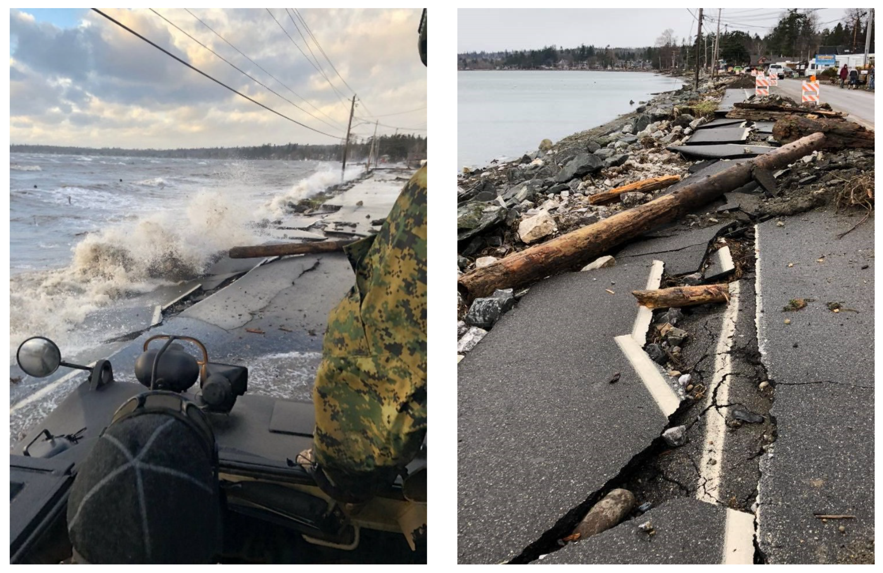
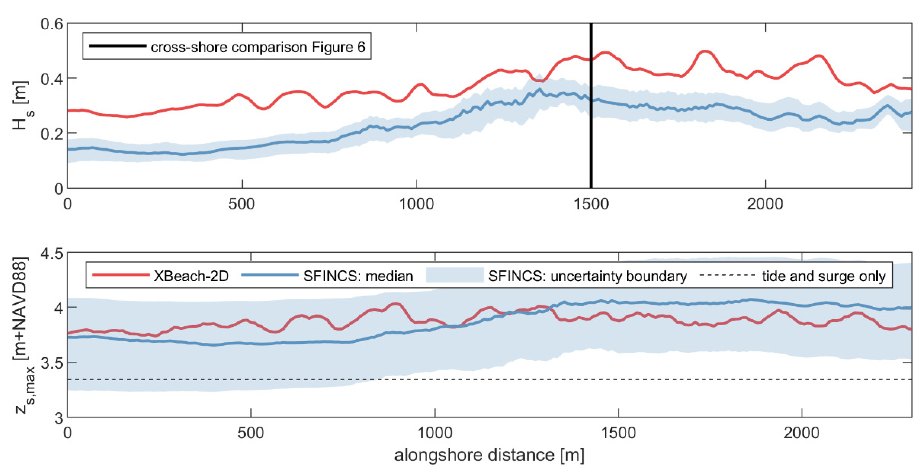
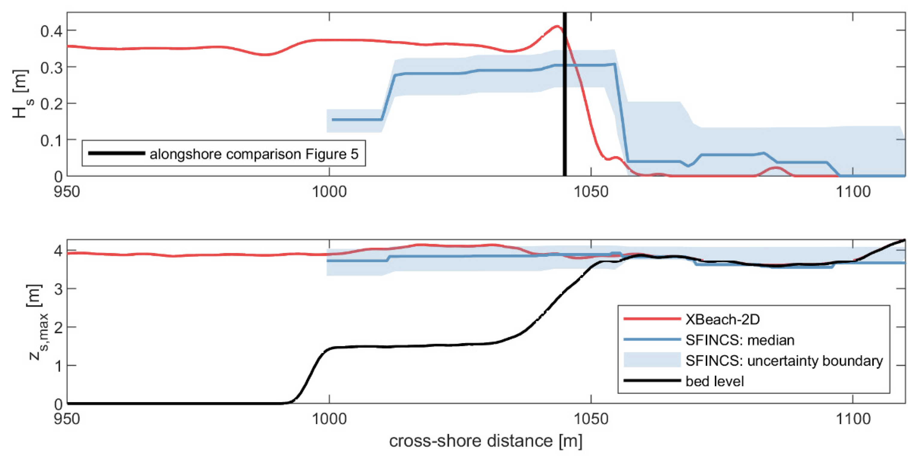
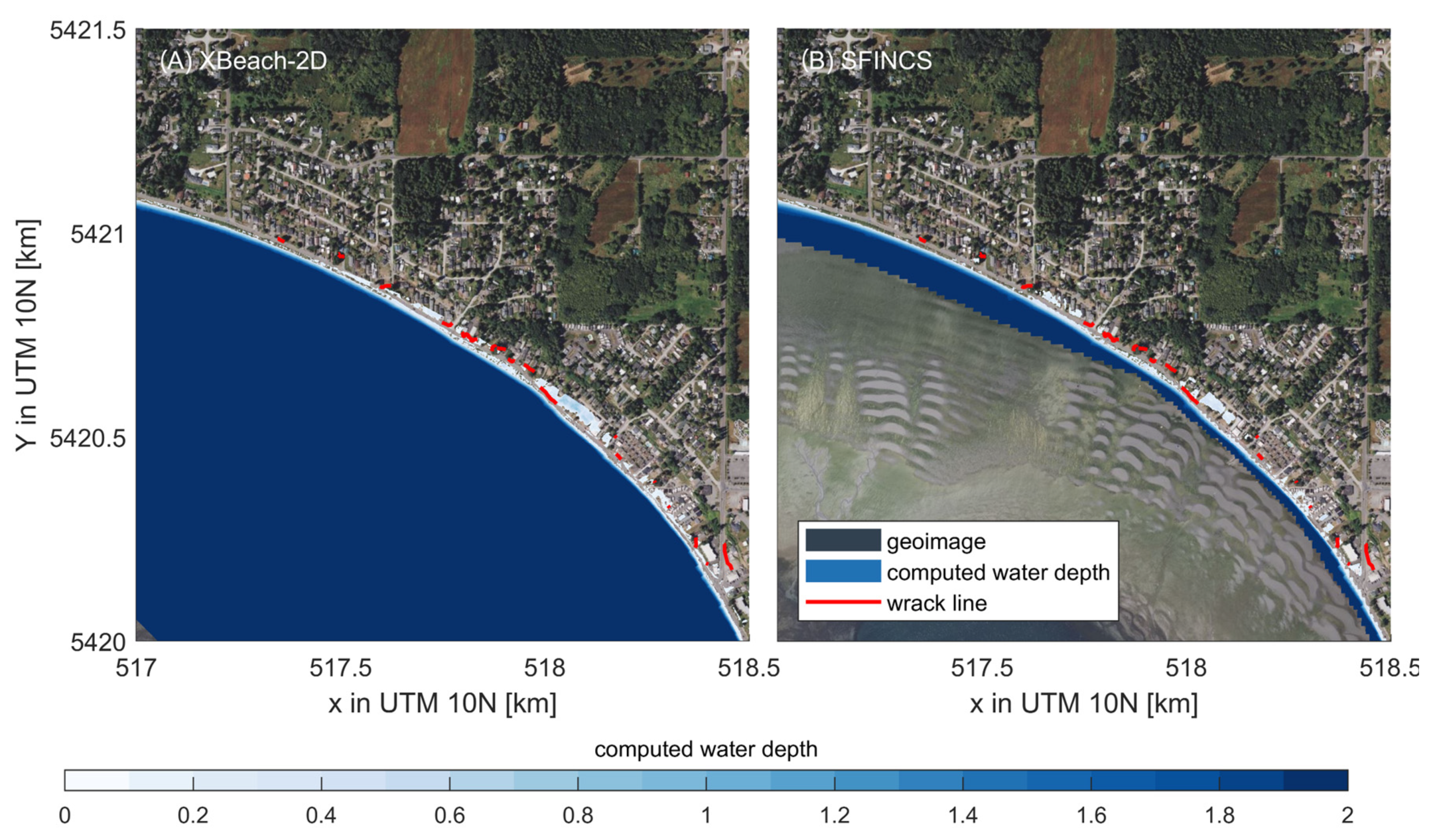
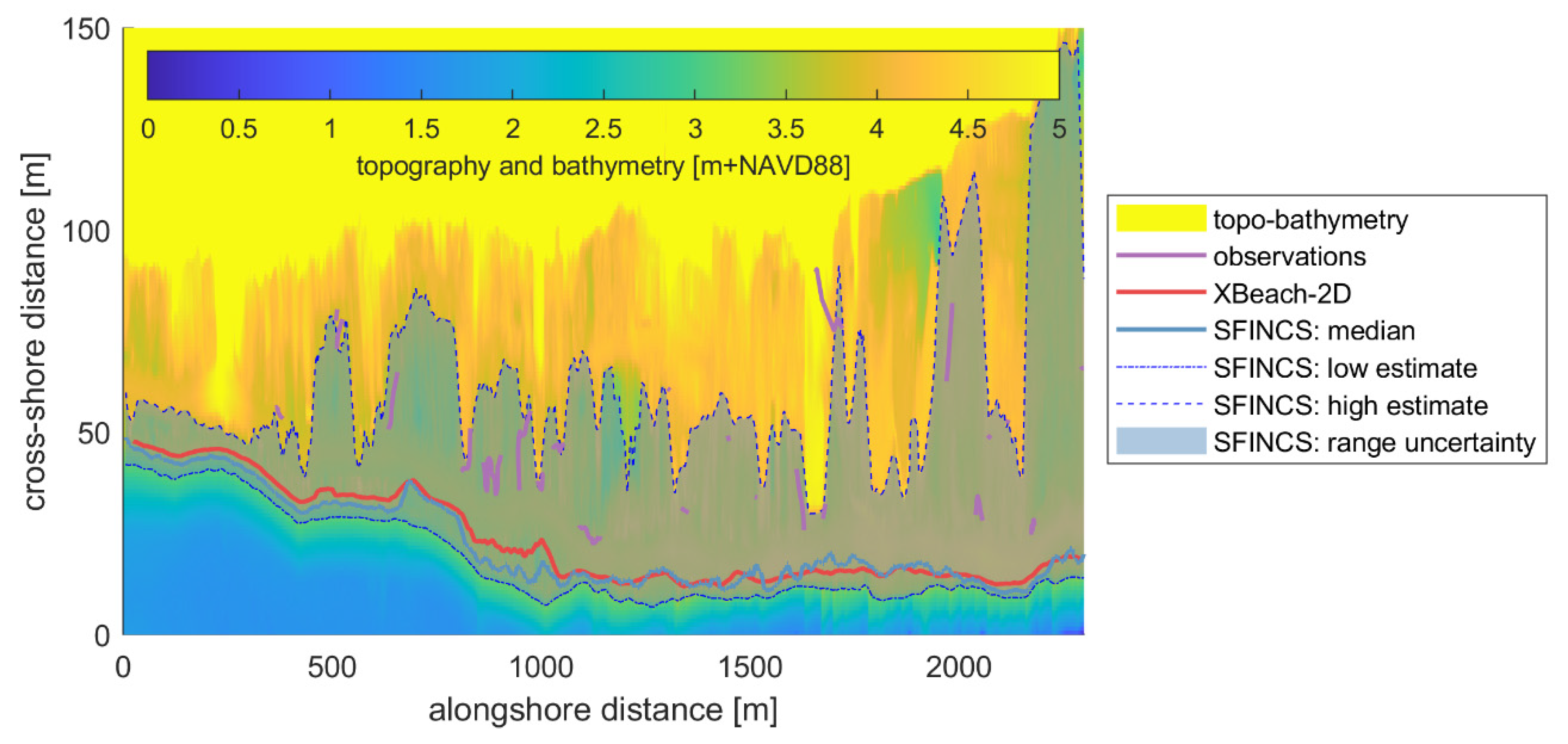
4.1. Validation: 20 December 2018, Event

For the validation study, model results from the SFINCS model for flood extent (2D comparison), wave height, total water level, and wave runup (all in alongshore direction) were compared to a computationally expensive two-dimensional XBeach-NH+ model (XB-2D) and observations based on wave runup. XBeach NH+ is used here as a reference model, since it includes all relevant physics to compute wave-driven flooding. Additional validation of the SFINCS results from domains 10, 11, 12 (see Figure 1 for their locations) comparing flood extents with the FEMA 1–100-year flood map can be found in Appendix A.

4.1.1. Overview

High tides in combination with wind-driven surges and waves, resulted in flooding landward of the Birch Bay Drive roadway in Birch Bay, Washington, on Thursday, 20 December 2018. The storm impacted all of Whatcom County, but the most severe impacts were observed in Birch Bay where significant road damage occurred, causing roads to remain closed for several weeks. Flooding and damage to homes, property, and infrastructure occurred along the entire waterfront of Birch Bay (Figure 3). Modeled still water levels in Birch Bay reached +3.3 m NAVD88 (Figure 4A) with predicted waves approaching 1.8 m in height and 4.5 s in their period (Figure 4B). Wind speeds reached ~20 m/s from the south to the west (Figure 4C).

Observations used for the model validation were based on a surveyed wrack line several days after the storm. The wrack line is a feature where material was deposited after the storm. In this paper, the wrack line is interpreted as the maximum wave runup extent (or maximum total water level) and used for validation purposes. However, the accuracy of a wrack-line-based estimate of wave runup is most likely relatively low, especially when compared to instrument-based observations of runup.

4.1.2. Computed Wave Height and Total Water Level

Figure 5 presents the alongshore-varying maximum modeled wave height (top panel) in ~1 m depth and the maximum total water level on land for the Birch Bay region during the storm of December 2018 for XBeach-2D (reference) and SFINCS (comparison). Alongshore variations in wave heights are similar between the XBeach 2D and SFINCS models with an RMSE of 12.2 cm. The discrepancy between the two models is largely driven by a bias of −11.7 cm (SFINCS underestimates compared to XBeach-2D). The total-water-level RMSE is 13.4 cm with a bias of −2.5 cm (bottom panel). Uncertainty in boundary conditions is included with a low and high estimate (−2 and + 2 standard deviations, 95% confidence interval; CI; see blue shading in Figure 5) and assumes normal uncorrelated unbiased errors. Uncertainty in boundary conditions of the SFINCS model are estimated to be 17 cm [20] and 12 cm [19] for wave heights and water levels, respectively. Thus, including the full range of boundary condition uncertainties shows that the errors made using simplifications in the model application framework are minor relative to uncertainty in the forcing conditions for predictions of overland flooding. Cross-shore computed wave heights and maximum water levels are presented in Figure 6. Again, wave heights tend to be underestimated using SFINCS compared to XBeach-2D. Moreover, the relatively coarse model resolution used in SFINCS is apparent by the mismatch of the moment of wave breaking. However, for the maximum, TWL SFINCS and XBeach-2D show similar patterns.

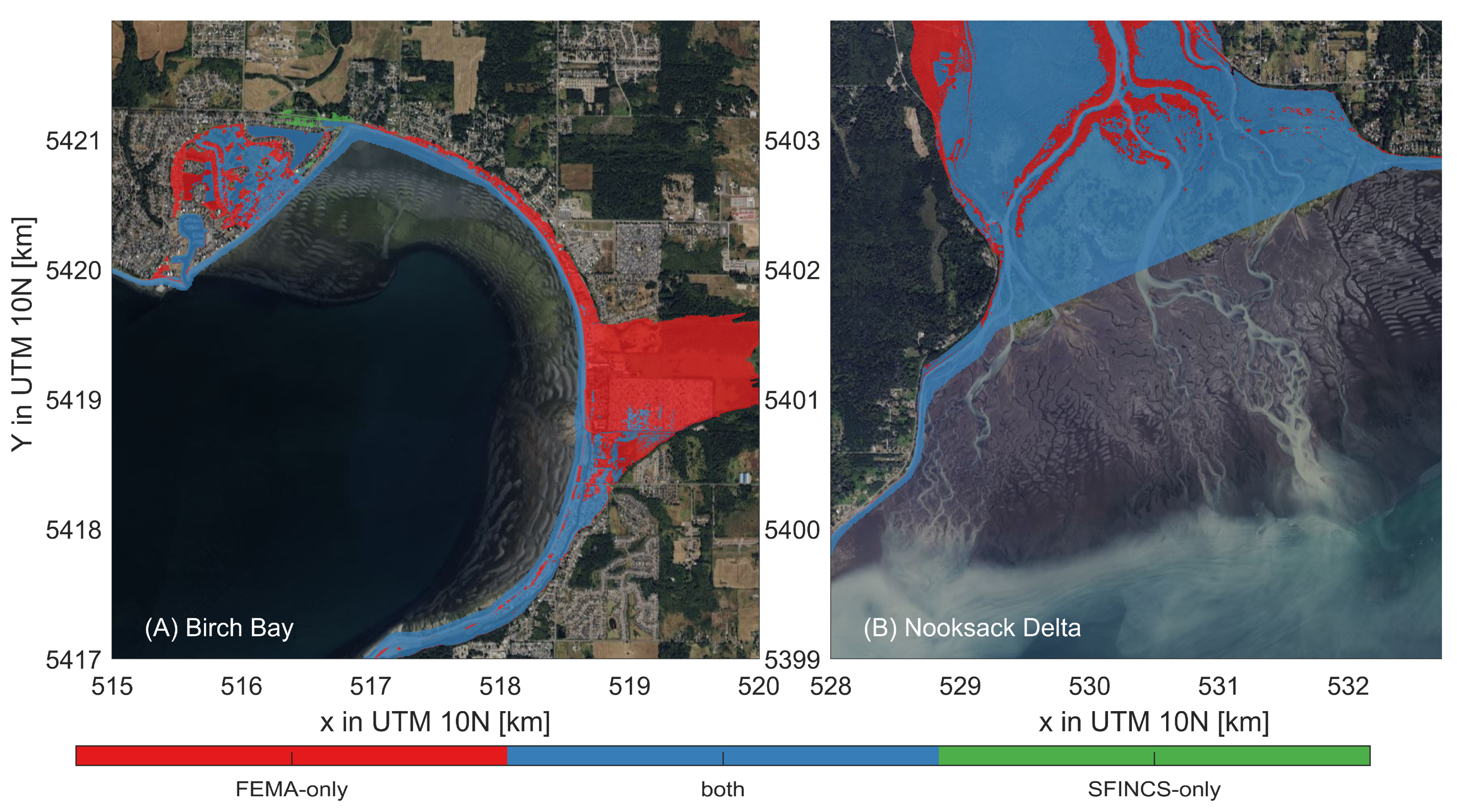
4.1.3. Flood Extent

For the Dec 2018 storm, the flood extents for both XB-2D and SFINCS are compared. Visually, the computed water depth using XB-2D and SFINCS match well when compared to the wrack line (Figure 7). Analyzing 407,005 1 × 1 m pixels for these models, shows a hit score of 0.80, indicating that 80% of the area flooded with the computationally expensive XB-2D model is reproduced using the reduced-complexity SFINCS model. The error bias is 0.46, indicating a tendency of underprediction using SFINCS. Only grid cells that are above 2 m NAVD88 and have at least 10 cm of water have been considered in this analysis. The difference in computational expense is a factor of 50,000 lower with SFINCS versus XB-2D (The two-dimensional XBeach-NH+ model (XB-2D) was run as a Linux cluster with 12 cores and took 311 hours to finish. SFINCS was run on a local Windows machine with 16 cores and took 21 seconds to finish. Directly dividing both computational expenses yields a speedup with SFINCS of 53,473 times. In this paper we reported 50,000 to account for the difference in the number of cores). Both simulations ran for 6 hr around the peak of the storm.

Models XB-2D and SFINCS are equally skillful in reproducing reconstructed high-water marks based on observed wrack lines (Figure 8). Model XB-2D reproduces the wave-driven runup length with a cross-shore RMSE of 29 m between runup toe and wrack line, while SFINCS has a RMSE of 30 m. In a relative sense, this results in a SCI of 59 and 63%, respectively. Both simulations have a substantial negative bias which indicates an underestimation of the flood extent compared to observations. It is unclear what the source of this underestimation is but it is suspected to be related to model bias in SWL due to underestimation of wind-driven setup. When comparing SFINCS with XB-2D, the wave-driven runup is well reproduced using the reduced-complexity model with an RMSD of 3.6 m compared to the XB-2D computed runup. The error is largely driven by a bias of −2.2 m (SFINCS underestimates compared to XB-2D). This bias is likely due to the lack of short-wave energy in SFINCS. Compared to the uncertainty of the boundary conditions, this seems acceptably small. In particular, the average difference in wave-driven runup as computed with SFINCS based on a low or high estimates of boundary conditions is ~50 m. In other words, the uncertainty using the model physics is an order of magnitude smaller compared to uncertainty in the forcing conditions. Qualitatively, the flood extent based on the high estimate matches reasonably well with the observed wrack line.

4.2. Projected Flood Hazards and Risks

In this section, model results for the future climate for several sea-level-rise scenarios are presented for the entire Whatcom County area of interest. First, the variability of the total water level is discussed. Secondly, flood hazards are presented and discussed. Lastly, we will discuss flood impacts across Whatcom County.

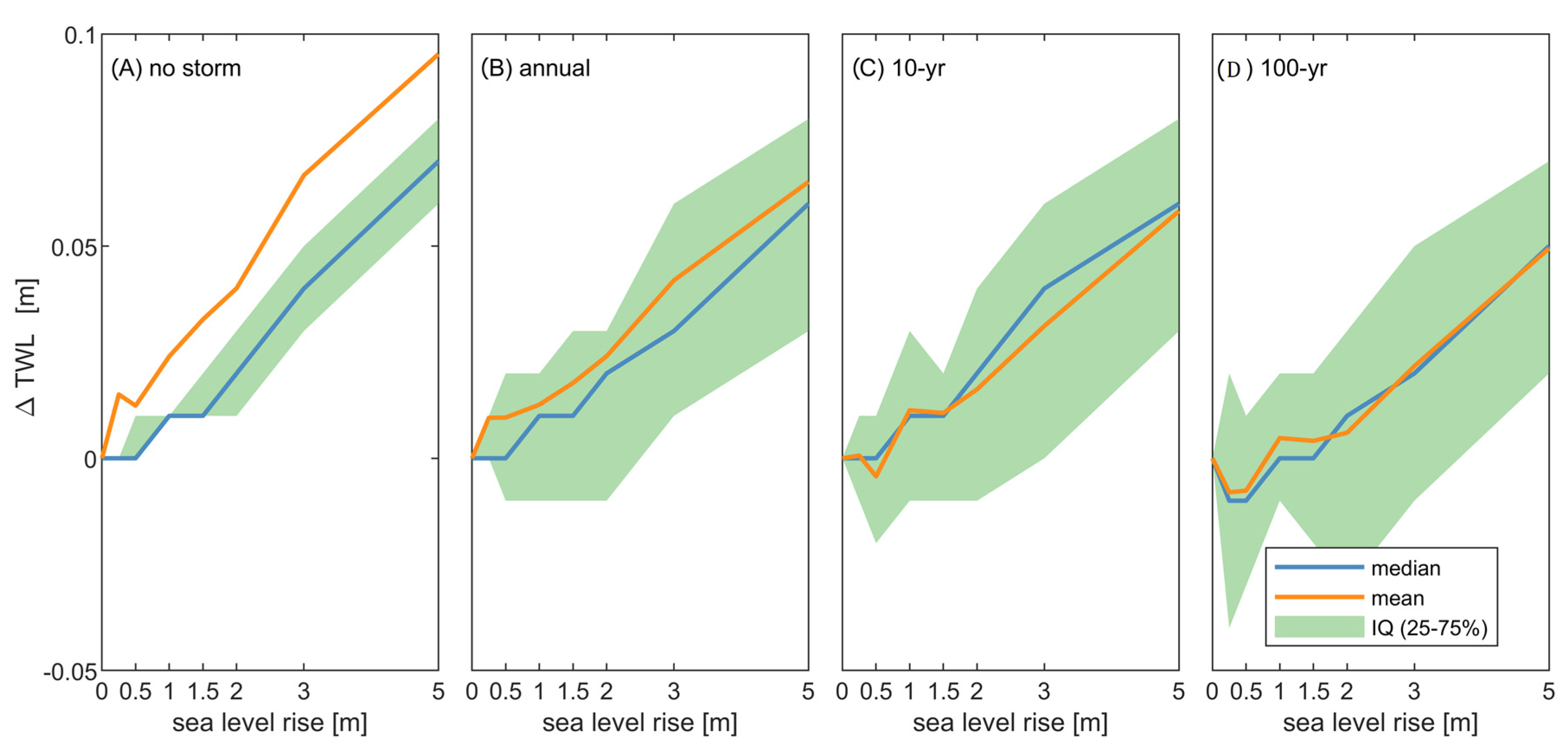
4.2.1. Total Water Level

Figure 9 presents the distribution of modeled maximum TWL for all analyzed grid cells for all SFINCS domains for the current sea level. TWL includes still water level (tide and surge) and wave-driven processes. TWL increases with the return period. For the no-storm conditions (Figure 9A), the interquartile range (IQ, red error bar) of TWL across Whatcom County is estimated to be +2.1–2.6 m NAVD88 (95% CI with a median of 2.4 m+NAVD88). This is close to a general tidal event and the background wave conditions add thus limited extra elevation. The 1–100-year IQ TWL is 1.2–1.3 m higher, has more variability, and reaches a median of 3.7 m+NAVD88. The quite large variability, for example, also shown by the 95% confidence interval, is strongly influenced by the dynamics on land. In particular, TWL at the coastline tends to be the highest and slowly dissipates due to friction on land. This cross-shore pattern of TWL shows the need for a process-based overland flooding model that includes relevant physics as compared to a simpler bathtub approach.

The change in maximum TWL as a function of sea-level rise for storms with return periods ranging from annual events to 100 year recurrence intervals illustrates their non-linearity (Figure 10). Here, the change in total water level (∆TWL) subtracts sea-level rise and, therefore, just shows the non-linearity. The value of ∆TWL increases with the increasing magnitude of SLR and for all SLR and storm return probabilities presented. This suggests that TWL is not a simple linear addition and that non-linearities between SLR, tide, waves, and wave runup are important to evaluate flood hazards across the study area accurately. For example, the TWL during the no-storm conditions increases for an SLR of 3 m between 3 and 5 cm (IQ; median 4 cm). This effect decreases for larger, less frequent storms. For example, the ∆TWL during the 1–100 year storm for SLR of 3 m is estimated to be 0 and 5 cm (IQ; median 3 cm). For most of the grid cells, the change is relatively minor (less than 10 cm), but important, in low-sloping areas. Note also the distance between mean and median which is <1 cm but does indicate a slight skewness in the distribution.

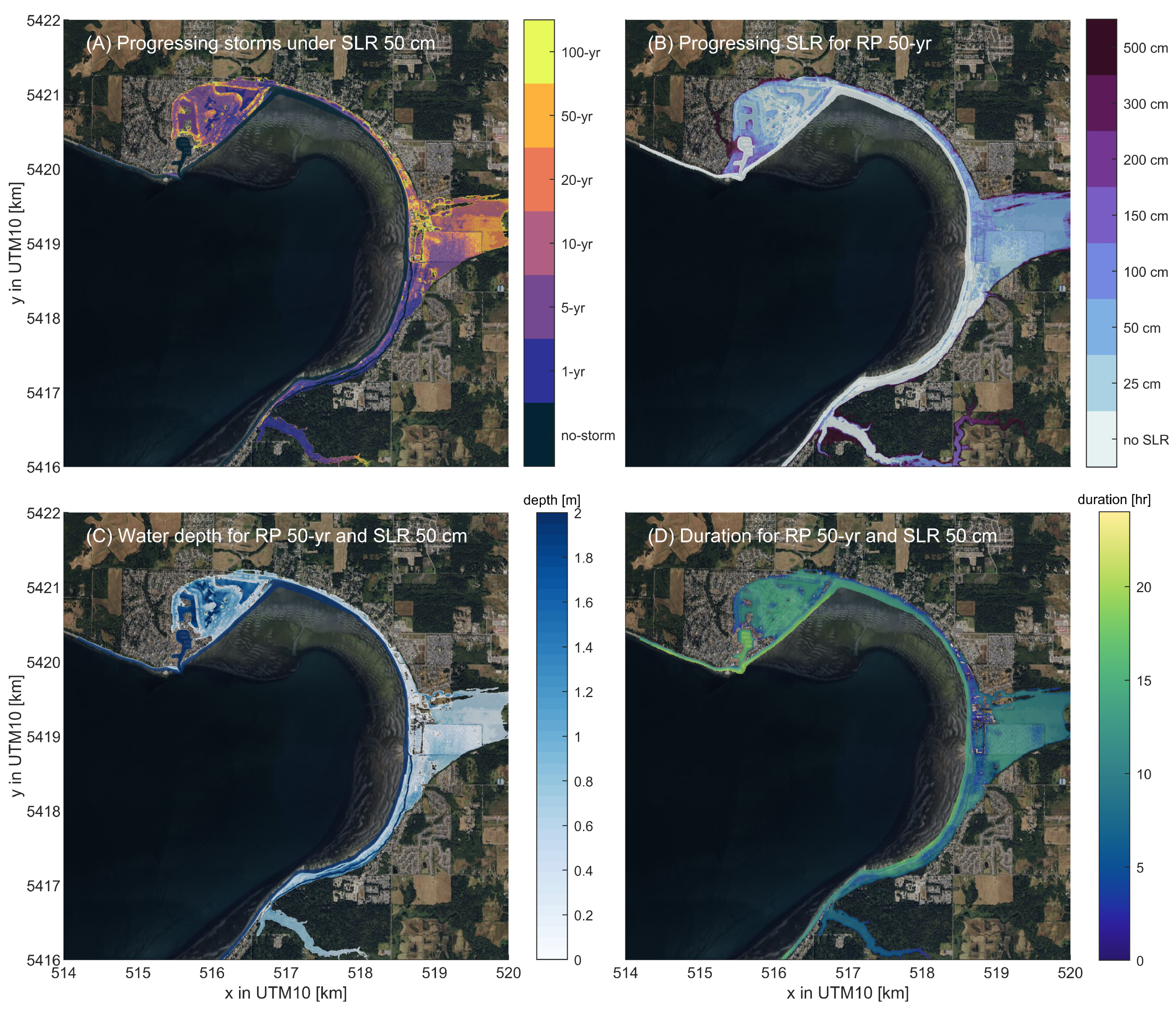
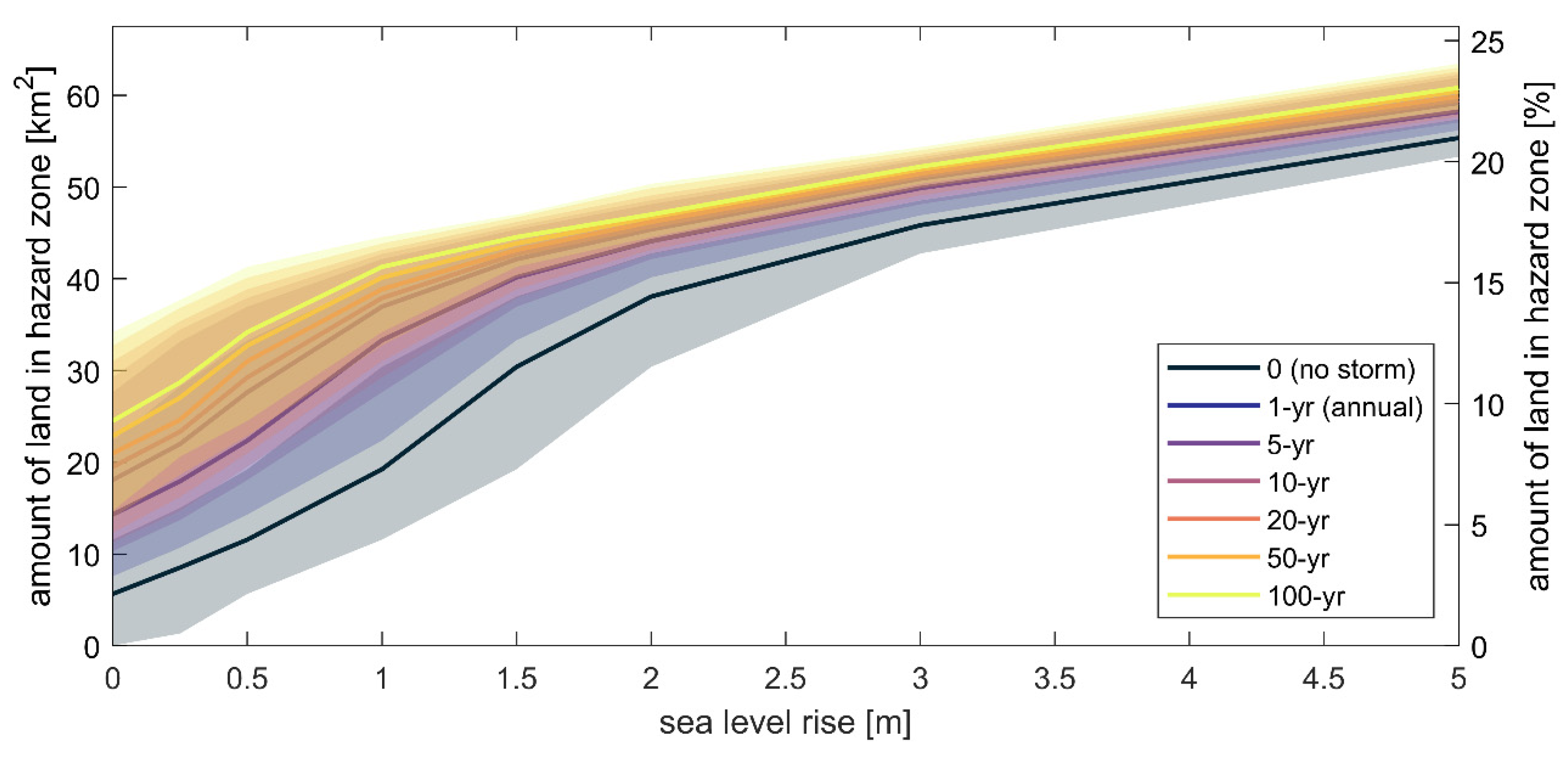
4.2.2. Flood Hazards

While flood hazards are calculated on a high spatial resolution (meter scale) for the entire Whatcom County shoreline, for clarity, we present these for a limited region around Birch Bay only as an example of the output (Figure 11). Panel A presents the range of flooding for progressively larger storm events for the sea-level-rise scenario of 50 cm with colors indicating a flooded grid cell and associated lowest return frequency. Panel B highlights the progressing effects of sea-level rise for a 50 year storm. The color represents which sea-level-rise scenario, a 1–50-year event (2% chance per year), results in flooding. Panel C shows the water depth for a return period of the 1–50-year event and the sea-level-rise scenario of 50 cm. Panel D presents the duration of the same 50 year flood event in hours with 50 cm of sea-level rise.

Figure 12 presents the flood extent in km² as a function of sea-level rise and storm frequency for grid cells above +2 m+NAVD88 within the coastal zone of Whatcom County (i.e., area of interest). Little to no inundation is projected with the no-storm condition and without sea-level rise as expected with a median TWL of 2.4 m NAVD88 (see Section ‘Total Water Level’). However, there is considerable uncertainty due to the error in the offshore water levels, wave height, and bathymetry. The area flooded under the 1–100-year storm scenario without sea-level rise encompasses ~24.5 km² which equates to 9% of the area of interest. With sea-level rise, these numbers are expected to increase. For the no-storm condition, the amount of area in the hazard zone almost linearly increases. In other words, for every 10 cm of sea-level rise, the amount of area in the hazard zone increases by ~1 km². The increase in hazard zone flooding for the storm conditions is less linear and is projected to taper off at higher sea levels. In particular, the increase in flooded area associated with the 1–100-year event with sea-level rise of 3 to 5 m is considerably less than the increase from 2 to 3 m sea-level rise. With 1 m of sea-level rise the yearly flood extent is projected to increase from 14 to 33 km² (5 and 13% of low-lying Whatcom County). These patterns are due to the unique topography in Whatcom County which is typically comprised of low-lying areas prone to coastal flooding that are backed by an abrupt change in elevation and showcasing the importance of site-specific coastal morphology for future flood hazard exposure.

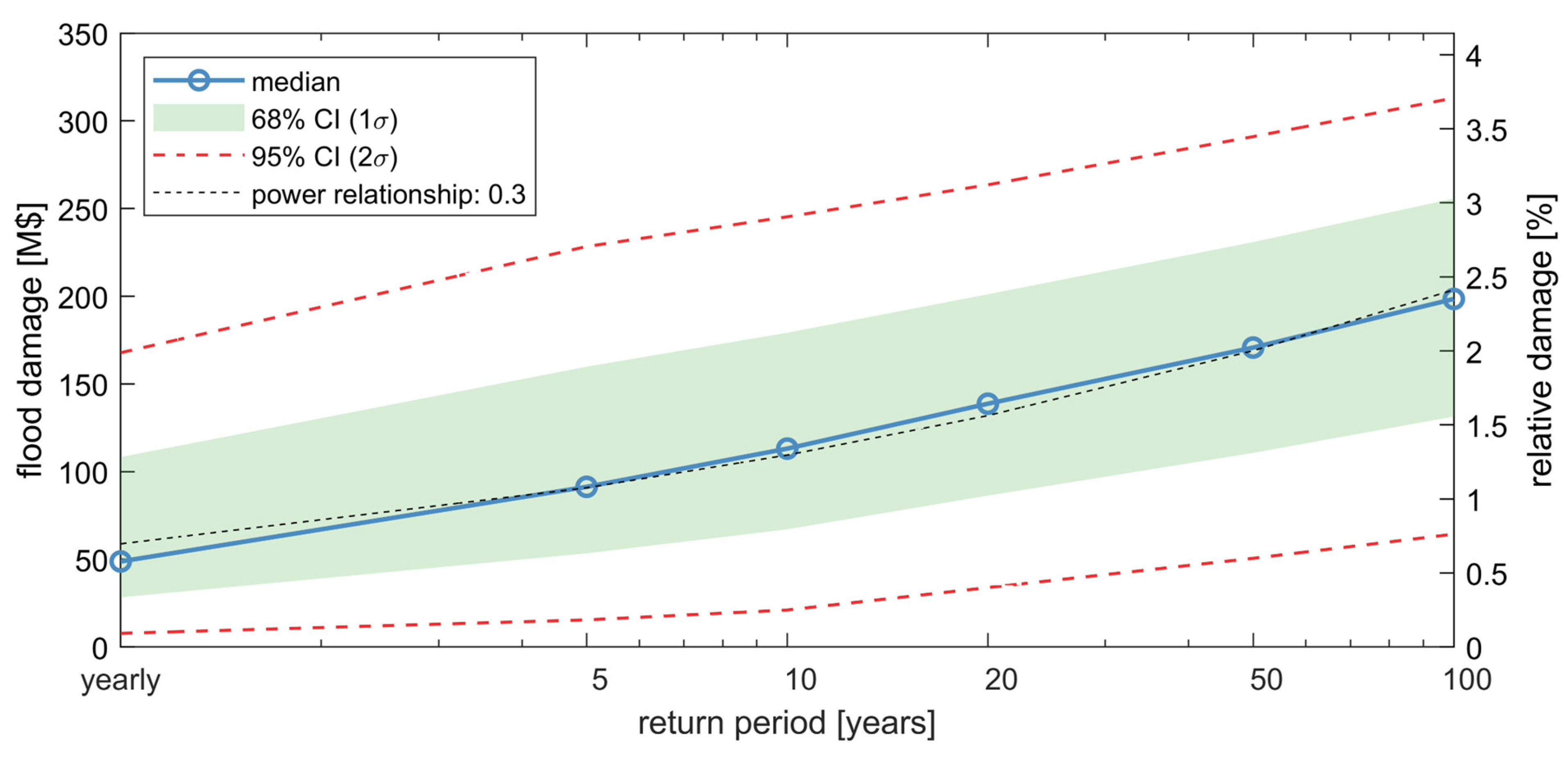
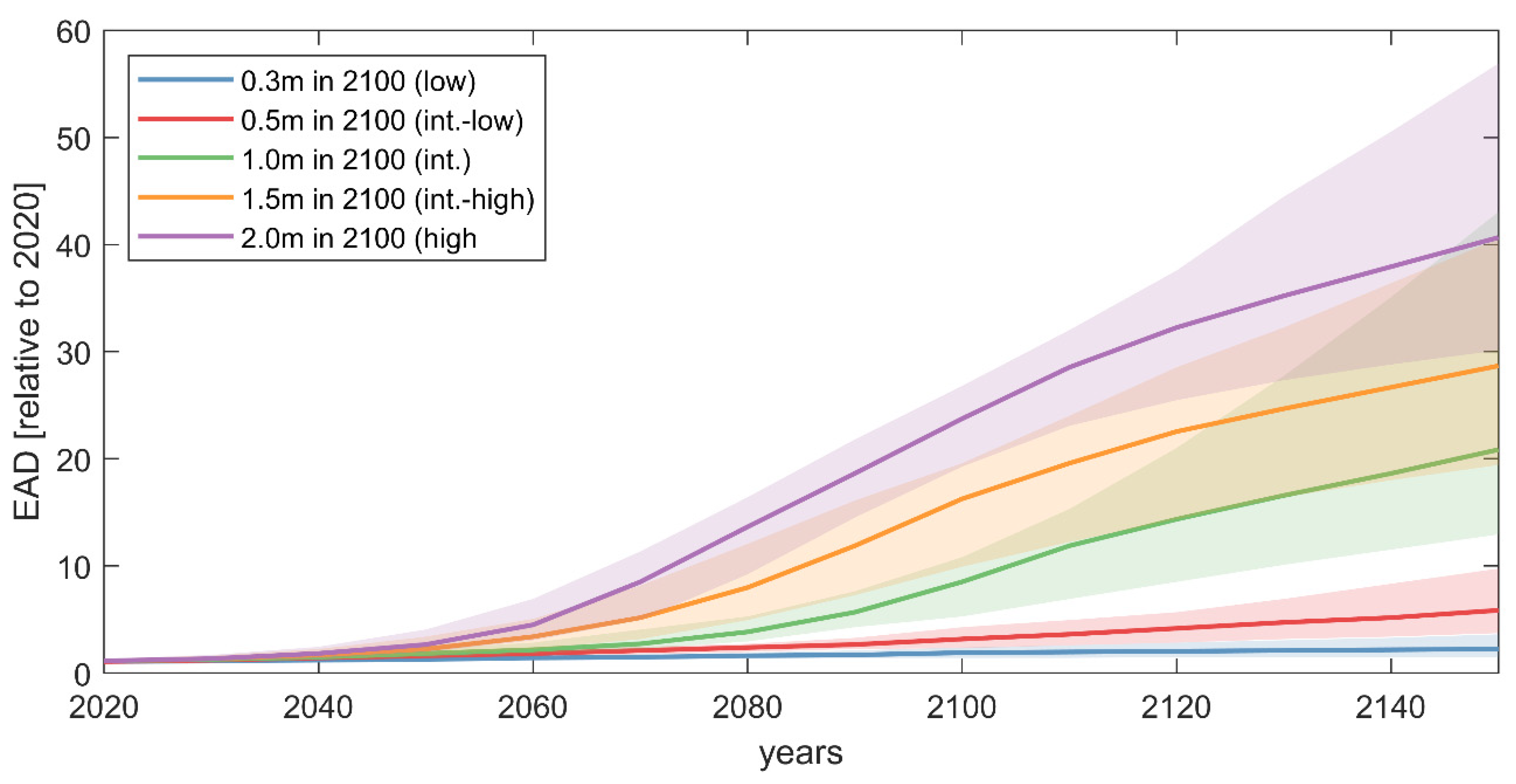
4.2.3. Flood Impact

Figure 13 presents the flood damages as computed per return period for coastal Whatcom County for 1.0 m of sea-level rise. Yearly flood damage for this sea-level-rise scenario is estimated to be between USD 29 and 108 million (1σ) for the current sea level. The large spread shows how sensitive the results are to the modeled flood depth, since the low estimate of damage uses the low estimate for flood hazard and uses it similarly for the high estimates. Median flood damage increases from USD 50 M to almost USD 200 M from yearly to the 100-year event. That is about 0.6 to 2.4% of the total value in the area analyzed. Damages tend to increase by a power of 0.3. In other words, a double of the return period will result in an (less than linear) increase.

By integrating the flood damages over the return period, it is possible to obtain a single estimate of the yearly flood risk. This is what is called Expected Annual Damages (EAD). EAD are estimated to increase from USD 14 M for the current sea level to USD 79 M, and USD 206 M and USD 320 M for sea-level rises of 0.5, 1.0, and 1.5 m. That is a fifteenfold increase for flood risk from the current sea level to 1 m of sea level.

With SLR, damage, risk, and number of affected people are expected to increase substantially (Figure 14). EAD computed for different sea-level-rise scenarios from [3] suggests that, depending on the specific scenario, flood risk in Whatcom County is expected to double sometime between 2040 and 2100 (using the median estimate) relative to today (e.g., not accounting for future economic development). For the medium scenario (1.0 m in 2100), a tenfold increase of flood risk is computed between 2100 and 2130 relative to current levels of exposure. The strong increase in flood risk is largely driven by the accelerating increase in projected mean sea level, since there is almost a linear relationship between risk and sea level.

5. Discussion

The validation presented here shows that PS-CoSMoS can reproduce the historically observed flooding at Birch Bay during the December 2018 storm with similar errors compared to the computationally expensive 2D XBeach implementation (Figure 5, Figure 6, Figure 7 and Figure 8). This has been achieved by using, first, an efficient regional hydrodynamic model to compute still water levels associated with tides and storm surges [19] and a regional wave model [20]. Secondly, skill and efficiency is achieved with a computational framework that uses LUT information from XB-NH+ transects for incoming (long period) waves in combination with the reduced-complexity SFINCS model for the overland flooding component. This approach allows for the simulation of hundreds of storm events with limited computational expense and, therefore, the possibility to determine compound flooding on a grid-cell-by-grid-cell basis for frequent and infrequent events. Therefore, PS-CoSMoS allows for the assessment of moderate disturbance events (e.g., the 1 and 20 year events), which can cumulatively outweigh the effects of only a 100 year event in the coming decades. However, we recognize that the validation strength of a single case study and flood feature like a wrack line where debris location likely underestimates the total extent of flooding by water, is limited. Therefore, we recommend that future work should focus on validation across other geographic areas and storm-event conditions

As part of the model validation, SFINCS-computed wave heights (Figure 5 and Figure 6), flooding (Figure 7), and runup (Figure 8) were underestimated compared to the computationally expensive two-dimensional non-hydrostatic XBeach-NH+ model. This is arguably due to the lack of short-period wave swash and, therefore, an underestimation of wave runup. SFINCS is forced with incoming waves via a LUT approach applied to 1D Xbeach transects. However, since shallow water equation solvers (such as SFINCS) have an accurate dispersion relationship for kh < 0.1, wave energy for periods shorter than 25 s were excluded from the incoming signal. Moreover, validation is performed for a limited geographic region within the larger model domain. Perhaps larger (or smaller) discrepancies would be noted if the validation was applied elsewhere. The reason for not including short-wave swash is the computational expense. Models such as XBeach-NH+ include the relevant physics. However, with the current computational resources, it is prohibitively expensive to apply this method for large stretches of coastline and for hundreds of storm events to account for compound flooding. The approach followed in this paper is ~50,000 times as efficient compared to XBeach-NH+ and, therefore, is chosen. The lack of suitable field data makes it impossible to (1) rigorously validate numerical models in Puget Sound for wave transformation, runup, and flooding and (2) to identify the dominant processes and sources of uncertainty.

Other (computationally efficient) approaches exist to estimate the effect of short waves on modeled flood extent. For example, Ref. [43] uses 1D profiles of XBeach in combination with LISFLOOD [44] where XBeach computes discharge time series of overtopping over the dune crest which is used as an input for LISFLOOD which computes the 2D flooding. The authors also included sandy morphodynamic change during the storm as part of the assessment. The current configuration of PS-CoSMoS uses a static DEM for both modeling of events and for flood projections. Several approaches exist to estimate the long-term shoreline development for open sandy coasts (e.g., [45]). However, to the knowledge of the authors, no such approach exists for sheltered complex estuaries or for areas with mixed-sediment glacially derived beach-setting characteristics like the Salish Sea. A comparison with the uncertainty of boundary conditions showed that the unreliability in the boundary forcing seems to be of larger importance than a simplification in physics (Figure 8). We argue that, for long-term planning, SLR projections, morphological change, and socio-economic uncertainty (e.g., exposure, water-depth–damage curve, population growth) are more important than incorporating all the relevant physical processes in the model framework [46]. Also, a comparison with the FEMA 100-year flood map for the current sea level shows a hit score of >80% which provides additional confidence in the PS-CoSMoS approach followed here (Appendix A) to inform planning decisions for diverse disturbance thresholds and timing in the coming decades.

In the current configuration, fluvial and pluvial processes are not considered at the same level of accuracy as coastal processes such as tides, surges, and waves. Due to a lack of concordant downscaled future hydrologic projections, a simplified daily averaged discharge cycle has been used for this study. Pluvial processes (i.e., precipitation/rainfall) were excluded. Moreover, no hydro-correction was applied to the DEM which might influence hydrologic connectivity. Historical examples (e.g., flooding of the Nooksack and Skagit Rivers in November 2021) and previous work (e.g., [11]) have suggested the importance of pluvial and fluvial drivers to compound flooding. This is expected to increase in importance with the projected increases in daily rainfall intensity associated with climate change in Washington State [7]. These sources of model inaccuracy also influence (and arguably underestimate) computed event duration. Further investigation is needed to assess the impacts of these drivers on flooding in the future climate as a result of changes in sea level and atmosphere. Improvements in the representation of fluvial, pluvial, and groundwater processes are steps we envision for future CoSMoS iterations.

Sea-level rise (SLR) affects flood hazards in multiple ways. First, through a linear increase in the offshore mean water level. Second, through non-linear effects on tides, surges, and waves (Figure 10). However, Ref. [19] showed the tidal amplitude and surge propagation pattern would not be altered in Birch Bay due to sea-level rise, while slight changes in tidal phase shift were predicted. Wave heights tend to increase along the shoreline with SLR due to a reduction in the dissipation from bottom friction. Model scenarios showed a strong increase in flood hazards and risk as a function of sea-level rise. These projections, however, are indicative of the potential effects but do not include local mitigation and adaptation. Adaptation will be dominant to the question of how flood hazards and risks develop in the future; however, these changes are not considered in this paper.

6. Conclusions

The Puget Sound Coastal Storm Modeling System (PS-CoSMoS) is a tool designed to dynamically downscale future climate scenarios and provide compound flood projections across large spatial scales at high resolution at the shore. The current configuration of CoSMoS accounts for tides, surges, waves, and winds associated with coastal processes that influence extreme water levels. Efforts are underway to also integrate the influence of pluvial, fluvial, and groundwater processes to improve forecasts of overland flooding. This manuscript introduced the compound flooding component which is based on the cross-shore-profile non-hydrostatic model XBeach and overland flooding model SFINCS. Via a novel wave transformation lookup table (LUT) of XBeach transect runs, it was possible to prescribe incoming wave energy along the SFINCS domains with limited computational expense. This method enables the computation of hundreds of storm events for dozens of sea-level-rise scenarios over a spatial scale of hundreds of kilometers and with the resolution required for planning purposes. The approach provides significantly more detailed flood exposure information and statistics for the combined effects of varying coastal storm recurrence and plausible sea-level rise up to 2100 accounting for uncertainty in boundary conditions and future projections.

Model validation showed that the SFINCS-based workflow can reproduce the main patterns observed during a historical extreme flood event, like in Birch Bay in 2018. Differences were found to be principally the result of uncertainty and underestimation of the large-scale boundary conditions and only partly due to the reduced modeling complexity of SFINCS. For the current sea level, flood hazards and risks are limited in Whatcom County. Flood exposure is expected to increase substantially with sea-level rise as the total water level increases in a non-linear manner. The yearly flood extent is projected to increase by 5 to 13% from the current level to a future 1 m sea-level rise. Flood risk is projected to increase fifteenfold for the same sea-level-rise scenario.

This paper introduces the model framework for overland compound flooding, including the application for Whatcom County. However, we plan to apply this framework for other areas across Puget Sound. The goal is the delivery of consistent, robust and authoritative SLR and storm impact projections at the local planning scale for the Salish Sea shorelines in the United States for the full range of plausible 21st-century SLR and storm scenarios.

References

- Munich, R. Natural Catastrophes 2021: Analyses, Assessments, Positions. 2022. Available online: https://www.munichre.com/en/company/media-relations/media-information-and-corporate-news/media-information/2021/2020-natural-disasters-balance.html (accessed on 1 August 2022).
- Easterling, D.R.; Meehl, G.A.; Parmesan, C.; Changnon, S.A.; Karl, T.R.; Mearns, L.O. Climate extremes: Observations, modeling, and impacts. Science 2000, 289, 2068–2074. [Google Scholar] [CrossRef] [PubMed]
- Sweet, W.V.; Hamlington, B.D.; Kopp, R.E.; Weaver, C.P.; Barnard, P.L.; Bekaert, D.; Craghan, M.; Dusek, G.; Frederikse, T.; Garner, G.; et al. Global and Regional Sea Level Rise Scenarios for the United States. NOAA Technical Report NOS 01. 2022; p. 111. Available online: https://oceanservice.noaa.gov/hazards/sealevelrise/sealevelrise-tech-report.html (accessed on 25 February 2022).
- Moftakhari, H.R.; AghaKouchak, A.; Sanders, B.F.; Feldman, D.L.; Sweet, W.; Matthew, R.A.; Luke, A. Increased nuisance flooding along the coasts of the United States due to sea level rise: Past and future. Geophys. Res. Lett. 2015, 42, 9846–9852. [Google Scholar] [CrossRef]
- Vitousek, S.; Barnard, P.; Fletcher, C.H.; Frazer, N.; Erikson, L.; Storlazzi, C.D. Doubling of coastal flooding frequency within decades due to sea-level rise. Sci. Rep. 2017, 7, 1399. [Google Scholar] [CrossRef] [PubMed]
- Tebaldi, C.; Ranasinghe, R.; Vousdoukas, M.; Rasmussen, D.J.; Vega-Westhoff, B.; Kirezci, E.; Kopp, R.E.; Sriver, R.; Mentaschi, L. Extreme sea levels at different global warming levels. Nat. Clim. Chang. 2021, 11, 746–751. [Google Scholar] [CrossRef]
- Mauger, G.S.; Casola, H.A.; Morgan, R.L.; Strauch, B.; Jones, B.; Curry, T.M. State of Knowledge: Climate Change in Puget Sound; Report prepared for the Puget Sound Partnership and the National Oceanic and Atmospheric Administration; Climate Impacts Group, University of Washington: Seattle, WA, USA, 2015. [Google Scholar] [CrossRef]
- Kron, W. Flood Risk = Hazard•Values•Vulnerability. Water Int. 2005, 30, 58–68. [Google Scholar] [CrossRef]
- NOAA. Sea Level Rise Viewer. 2022. Available online: https://coast.noaa.gov/slr/#/layer/slr (accessed on 22 February 2022).
- Barnard, P.L.; van Ormondt, M.; Erikson, L.H.; Eshleman, J.; Hapke, C.; Ruggiero, P.; Adams, P.N.; Foxgrover, A.C. Development of the Coastal Storm Modeling System (CoSMoS) for predicting the impact of storms on high-energy, active-margin coasts. Nat. Hazards 2014, 74, 1095–1125. [Google Scholar] [CrossRef]
- Wahl, T.; Jain, S.; Bender, J.; Meyers, S.D.; Luther, M.E. Increasing risk of compound flooding from storm surge and rainfall for major US cities. Nat. Clim. Chang. 2015, 5, 1093–1097. [Google Scholar] [CrossRef]
- O’Neill, A.C.; Erikson, L.H.; Barnard, P.L. Downscaling wind and wavefields for 21st century coastal flood hazard projections in a region of complex terrain. Earth Space Sci. 2017, 4, 314–334. [Google Scholar] [CrossRef]
- O’Neill, A.; Erikson, L.H.; Barnard, P.L.; Limber, P.W.; Vitousek, S.; Warrick, J.A.; Foxgrover, A.C.; Lovering, J. Projected 21st Century Coastal Flooding in the Southern California Bight. Part 1: Development of the Third Generation CoSMoS Model. J. Mar. Sci. Eng. 2018, 6, 59. [Google Scholar] [CrossRef]
- United States Census Bureau 2020 Population and Housing State Data for Whatcom County, WA. 2020. Available online: http://censusreporter.org/profiles/05000US53073-whatcom-county-wa (accessed on 11 July 2022).
- Finlayson, D. The Geomorphology of Puget Sound Beaches. Puget Sound Nearshore Partnership Technical Report 2006-02, no. October. 2006, p. 56. Available online: http://oai.dtic.mil/oai/oai?verb=getRecord&metadataPrefix=html&identifier=ADA477465 (accessed on 11 July 2022).
- Mass, C. The Weather of the Pacific Northwest; University of Washington Press: Seattle, WA, USA, 2008; ISBN 978-0-295-98847-4. [Google Scholar]
- Soontiens, N.; Allen, S.E.; Latornell, D.; Le Souëf, K.; Machuca, I.; Paquin, J.P.; Lu, Y.; Thompson, K.; Korabel, V. Storm Surges in the Strait of Georgia Simulated with a Regional Model. Atmos.-Ocean 2016, 54, 1–21. [Google Scholar] [CrossRef]
- Yang, Z.; García-Medina, G.; Wu, W.C.; Wang, T.; Leung, L.R.; Castrucci, L.; Mauger, G. Modeling analysis of the swell and wind-sea climate in the Salish Sea. Estuar. Coast. Shelf Sci. 2019, 224, 289–300. [Google Scholar] [CrossRef]
- Grossman, E.E.; Tehranirad, B.; Nederhoff, C.M.; Crosby, S.C.; Stevens, A.W.; Van Arendonk, N.R.; Nowacki, D.J.; Erikson, L.H.; Barnard, P.L. Modeling Extreme Water Levels in the Salish Sea: The Importance of Including Remote Sea Level Anomalies for Application in Hydrodynamic Simulations. Water 2023, 15, 4167. [Google Scholar] [CrossRef]
- Crosby, S.C.; Nederhoff, K.; VanArendonk, N.; Grossman, E.E. Efficient modeling of wave generation and propagation in a semi-enclosed estuary. Ocean Model. 2023, 184, 102231. [Google Scholar] [CrossRef]
- Roelvink, D.; Mccall, R.; Mehvar, S.; Nederhoff, K.; Dastgheib, A. Improving predictions of swash dynamics in XBeach: The role of groupiness and incident-band runup. Coast. Eng. 2018, 134, 103–123. [Google Scholar] [CrossRef]
- Roelvink, D.; Reniers, A.J.H.M.; van Dongeren, A.; van Thiel de Vries, J.S.M.; McCall, R.T.; Lescinski, J. Modelling storm impacts on beaches, dunes and barrier islands. Coast. Eng. 2009, 56, 1133–1152. [Google Scholar] [CrossRef]
- Leijnse, T.; van Ormondt, M.; Nederhoff, K.; van Dongeren, A. Modeling compound flooding in coastal systems using a computationally efficient reduced-physics solver: Including fluvial, pluvial, tidal, wind- and wave-driven processes. Coast. Eng. 2021, 163, 103796. [Google Scholar] [CrossRef]
- Kernkamp, H.W.J.; van Dam, A.; Stelling, G.S.; de Goede, E.D. Efficient scheme for the shallow water equations on unstructured grids with application to the Continental Shelf. Ocean. Dyn. 2011, 61, 1175–1188. [Google Scholar] [CrossRef]
- Tyler, D.J.; Danielson, J.J.; Grossman, E.E.; Hockenberry, R.J. Topobathymetric Model of Puget Sound, Washington, 1887 to 2017: U.S. Geological Survey Data Release. 2020. Available online: https://www.sciencebase.gov/catalog/item/5d72b5dfe4b0c4f70cffa775 (accessed on 11 July 2022).
- Homer, C.; Dewitz, J.; Jin, S.; Xian, G.; Costello, C.; Danielson, P.; Gass, L.; Funk, M.; Wickham, J.; Stehman, S.; et al. Conterminous United States land cover change patterns 2001–2016 from the 2016 National Land Cover Database. ISPRS J. Photogramm. Remote Sens. 2020, 162, 184–199. [Google Scholar] [CrossRef]
- Nederhoff, K.; Saleh, R.; Tehranirad, B.; Herdman, L.; Erikson, L.; Barnard, P.L.; Van der Wegen, M. Drivers of extreme water levels in a large, urban, high-energy coastal estuary—A case study of the San Francisco Bay. Coast. Eng. 2021, 170, 103984. [Google Scholar] [CrossRef]
- Mass, C.F.; Salathé, E.P.; Steed, R.; Baars, J. The Mesoscale Response to Global Warming over the Pacific Northwest Evaluated Using a Regional Climate Model Ensemble. J. Clim. 2022, 35, 2035–2053. [Google Scholar] [CrossRef]
- Nowacki, D.; Stevens, A.; Vanarendonk, N.R.; Grossman, E. Time-Series Measurements of Pressure, Conductivity, Temperature, and Water Level Collected in Puget Sound and Bellingham Bay, Washington, USA, 2018 to 2021: U.S. Geological Survey Data Release. 2021. Available online: https://cmgds.marine.usgs.gov/data-releases/datarelease/10.5066-P9JTFJ6M/ (accessed on 11 July 2022).
- Booij, N.; Ris, R.C.; Holthuijsen, L.H. A third-generation wave model for coastal regions. I-Model description and validation. J. Geophys. Res. 1999, 104, 7649–7666. [Google Scholar] [CrossRef]
- Hamlet, A.F.; Elsner, M.M.G.; Mauger, G.S.; Lee, S.Y.; Tohver, I.; Norheim, R.A. An overview of the columbia basin climate change scenarios project: Approach, methods, and summary of key results. Atmos.-Ocean 2013, 51, 392–415. [Google Scholar] [CrossRef]
- de Bruijn, K.M. Resilience and Flood Risk Management: A Systems Approach Applied to Lowland Rivers; Delft University Press: Delft, The Netherlands, 2005; ISBN 90-407-2599-3. [Google Scholar]
- Esch, T.; Heldens, W.; Hirner, A.; Keil, M.; Marconcini, M.; Roth, A.; Zeidler, J.; Dech, S.; Strano, E. Breaking new ground in mapping human settlements from space—The Global Urban Footprint. ISPRS J. Photogramm. Remote Sens. 2017, 134, 30–42. [Google Scholar] [CrossRef]
- Florczyk, A.J.; Freire, S.; Corbane, C.; Zanchetta, L.; Schiavina, M.; Politis, P.; Kemper, T.; Ehrlich, D.; Pesaresi, M.; Maffenini, L.; et al. GHSL Data Package 2019; Publications Office: 2019. Available online: https://op.europa.eu/en/publication-detail/-/publication/ce98358f-1a32-11ea-8c1f-01aa75ed71a1/language-en (accessed on 11 July 2022).
- Huizinga, J.; de Moel, H.; Szewczyk, W. Global Flood Depth-Damage Functions; Publications Office: 2017. Available online: https://op.europa.eu/en/publication-detail/-/publication/a20ecfa5-200e-11e7-84e2-01aa75ed71a1/language-en (accessed on 11 July 2022).
- de Ridder, M.P.; Smit, P.B.; van Dongeren, A.; McCall, R.T.; Nederhoff, K.; Reniers, A.J.H.M. Efficient two-layer non-hydrostatic wave model with accurate dispersive behaviour. Coast. Eng. 2021, 164, 103808. [Google Scholar] [CrossRef]
- Leijnse, T.; Nederhoff, K.; van Dongeren, A.; McCall, R.T.; van Ormondt, M. Improving computational efficiency of compound flooding simulations: The SFINCS model with subgrid features. In AGU Fall Meeting Abstracts; 2020; Volume 2020, p. NH022-0006. Available online: https://ui.adsabs.harvard.edu/abs/2020AGUFMNH0220006L/abstract (accessed on 11 July 2022).
- Athif, A.A. Computationally efficient modelling of wave driven flooding in Atoll Islands. IHE Delft 2020. [Google Scholar] [CrossRef]
- Stockdon, H.F.; Holman, R.A.; Howd, P.A.; Sallenger, A.H. Empirical parameterization of setup, swash, and runup. Coast. Eng. 2006, 53, 573–588. [Google Scholar] [CrossRef]
- Makkonen, L. Plotting positions in extreme value analysis. J. Appl. Meteorol. Climatol. 2007, 46, 396. [Google Scholar] [CrossRef]
- Weibull, W. A statistical theory of strength of materials. Ing. Vetensk. Akad. Handl. 1939. [Google Scholar]
- Wing, O.E.J.; Bates, P.D.; Sampson, C.C.; Smith, A.M.; Johnson, K.A.; Erickson, T.A. Validation of a 30 m resolution flood hazard model of the conterminous United States. Water Resour. Res. 2017, 53, 7968–7986. [Google Scholar] [CrossRef]
- Armaroli, C.; Duo, E.; Viavattene, C. From Hazard to Consequences: Evaluation of Direct and Indirect Impacts of Flooding Along the Emilia-Romagna Coastline, Italy. Front. Earth Sci. 2019, 7, 1–20. [Google Scholar] [CrossRef]
- Bates, P.D.; Horritt, M.S.; Fewtrell, T.J. A simple inertial formulation of the shallow water equations for efficient two-dimensional flood inundation modelling. J. Hydrol. 2010, 387, 33–45. [Google Scholar] [CrossRef]
- Bruun, P. Coastal Erosion and the Development of Beach Profiles; U.S. Army Corps of Engineers Beach Erosion Board Technical Memo, 1954; Volume 44. Available online: https://hdl.handle.net/11681/3426 (accessed on 11 July 2022).
- Parodi, M.U.; Giardino, A.; van Dongeren, A.; Pearson, S.G.; Bricker, J.D.; Reniers, A.J.H.M. Uncertainties in coastal flood risk assessments in small island developing states. Nat. Hazards Earth Syst. Sci. 2020, 20, 2397–2414. [Google Scholar] [CrossRef]
- Grossman, E.E.; Tehranirad, B.; Stevens, A.W.; VanArendonk, N.R.; Crosby, S.; Nederhoff, K. Salish Sea Hydrodynamic Model: U.S. Geological Survey Data Release. 2023. Available online: https://www.sciencebase.gov/catalog/item/63a0ae08d34e0de3a1f277a0 (accessed on 11 July 2022).