A Pragmatic Approach for Chlorine Decay Modeling in Multiple-Source Water Distribution Networks Based on Trace Analysis

Abstract

Providing water with adequate quality to users is one of the main concerns for water utilities. In most countries, this is ensured through the introduction of disinfectants, such as chlorine, which are subjected to decay over time, with consequent loss of disinfection action and the possible formation of harmful by-products. In this context, water quality models can be a useful tool to support management and, thus, ensure sufficient standards in all network points, but most of these models require the input of reaction parameters which could be difficult to obtain based on the information available to water utilities, especially in the case of complex water distribution networks (WDNs) supplied by more than one source. This study proposes a pragmatic, interval-number-based method to model chlorine decay in complex WDNs by relying on the use of the network hydraulic model and the results of trace analysis, which are exploited to obtain overall reaction rates. The method is applied to the case of a real WDN supplied by water sources with different qualitative features. The results obtained highlight that the method can help water utilities in the identification of overall water quality parameters.

1. Introduction

Ensuring high qualitative standards of drinking water at the user’s tap is essential in preserving human health [1,2]. However, this challenge is currently threatened by freshwater scarcity and pollution of water bodies. A major consequence of the poor management of drinking water or the entry of contaminants into networks is the outbreaks of disease that can affect especially fragile individuals, e.g., children and the elderly [3]. Although drinking water standards tend to vary worldwide, a common principle is that actions aimed at reducing contaminants to levels that are not harmful to health must be taken on several fronts—i.e., from the source to the user’s tap—based on drinking water characteristics which, in turn, depend on the characteristics of the water source [4].

Independently of the characteristics of drinking water, it is clear that the control and reduction of pathogenic microorganisms in water distribution networks (WDNs) is essential. In most cases, this is ensured by using reactive chemical agents, such as chlorine products [5], although this is not the only solution [6]. With regard to the former case, because water quality decreases as water travels through pipes, a general rule to constantly ensure sufficient quality is to reduce the residence time of water in the network (i.e., water age) [7]. In fact, an excessive water age can determine the reduction of free residual chlorine and the formation of harmful chlorination by-products [2,8]. In addition, high water age can also result in low velocities through pipelines and, in particular, the failure to reach the daily self-cleaning velocity [9,10,11]. This is more often observed in strongly looped WDNs, whereas branched systems generally tend to experience sufficient water velocity in pipes to ensure an acceptable residual chlorine concentration (RCC) [12,13].

From an operational standpoint, water quality controls are aimed at ensuring that drinking water meets the requirements imposed by global and local regulation systems. Controls are generally performed both at the source and in proximity to various sampling points within the WDN, in order to monitor RCC in water [14], which is a good surrogate indicator of water quality [15]. According to the World Health Organization, the optimal suggested value is 0.2 mg/L, whereas maximum concentrations should not exceed 0.5 mg/L [16]. In this context, increasingly strict regulations are leading water utilities to make use of support tools like water quality models to obtain insights into the spatial and temporal distribution of water quality indicators (e.g., RCC) in WDNs [17]. In general, water quality models can be used for several purposes aimed at improving the performance of pre-existing systems or supporting the design of new WDNs, such as: ensuring an adequate RCC in all network points (even in those located in more disadvantaged areas), reducing water age in the network to avoid the formation of harmful by-products, and optimizing the placement of chlorine boosters [18,19]. In light of the above, recent research in the literature includes studies about the topic of water quality modeling and, in particular, the modeling of chlorine decay. However, most of these studies focus on WDNs featuring a very simplified layout and generally supplied by a single source (e.g., Refs. [20,21]). Therefore, the current literature lacks examples of chlorine decay model applications to complex networks supplied by different sources with different water quality characteristics, as in typical cases of WDNs managed by water utilities. In addition, it has to be highlighted that chlorine decay models are generally based on rather complex approaches [21,22,23,24], the application of which requires detailed water quality parameters that may be hard to obtain for water utilities [25] even in the case of simple WDN layouts. Indeed, these depend on both water characteristics (e.g., water pH and temperature, affecting bulk reaction parameters) and pipe characteristics (i.e., material and age, affecting wall reaction parameters) and should be obtained for each individual network pipeline based on the results of laboratory tests [23,26].

In an effort to make an innovative contribution to the available literature, this study proposes an approach to model water quality in WDNs, aimed at addressing the following research question: How do we face the problem of chlorine decay modeling in complex WDNs, supplied by several sources featuring water of different qualitative characteristics by exclusively exploiting RCC data collected in the field?

In the light of the above question, this study proposes a pragmatic method which relies on an interval-number-based approach to model chlorine decay in complex WDNs. In greater detail, interval numbers are exploited to describe the overall reaction rates (including contributions from both bulk and the wall reactions) based on the use of the network hydraulic model and trace analysis results. Compared to the methods available in the literature on the topic, the proposed approach provides a novel contribution due to its pragmatic nature, which allows the application to complex, multiple-source WDNs and not only to simple WDN layouts such as those typically considered when dealing with water quality modeling. Method effectiveness is tested in relation to a real case study including a complex, looped, and multiple-source system, for which the continuous, real-time sampling of chlorine concentration has been performed at several points within the WDN.

In the following sections, the layout of the developed methodology and the real WDN assumed as a case study are presented, along with a discussion of field data collected and considered to test the method (Section 2). The results obtained are then shown and discussed (Section 3). Lastly, study limitations and requirements are given (Section 4) and the main outcomes of the study are provided (Section 5).

2. Materials and Methods

In the following, the methodology aimed at the modeling of chlorine decay in complex WDNs is described, along with the characteristics of the real WDN considered as a case study—and to which the developed methodology is applied—and the field RCC data available.

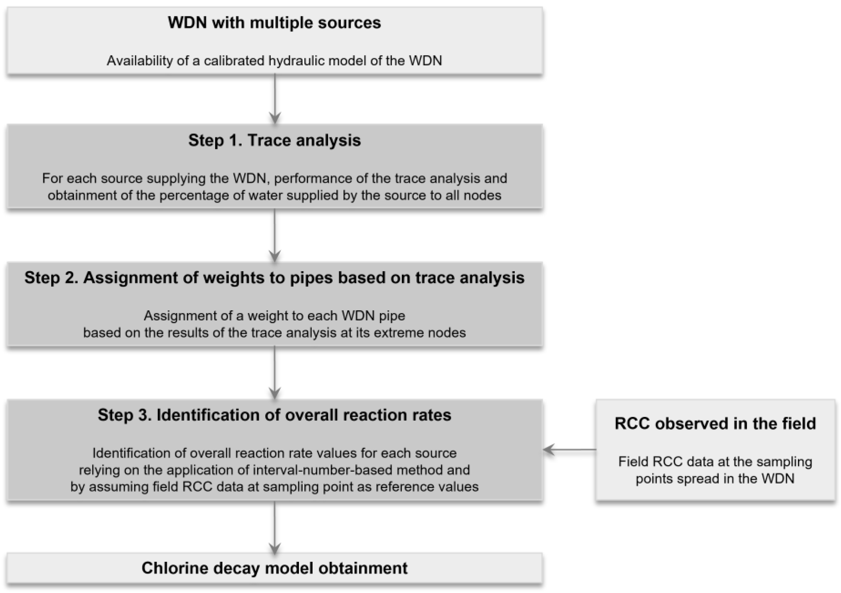
2.1. Methodology

The methodology proposed in this study, the layout of which is shown in Figure 1, is structured in three steps. The method is here presented in relation to a generic WDN characterized by $n_N$ nodes (i.e., junctions), $n_L$ links (i.e., pipes) and $n_S$ sources, and for which the hydraulic model is available. Let us assume that RCC data are collected with a given temporal resolution (e.g., 1 h) at $n_P$ sampling points spread all over the WDN, for a sufficiently long period (e.g., 1 year).

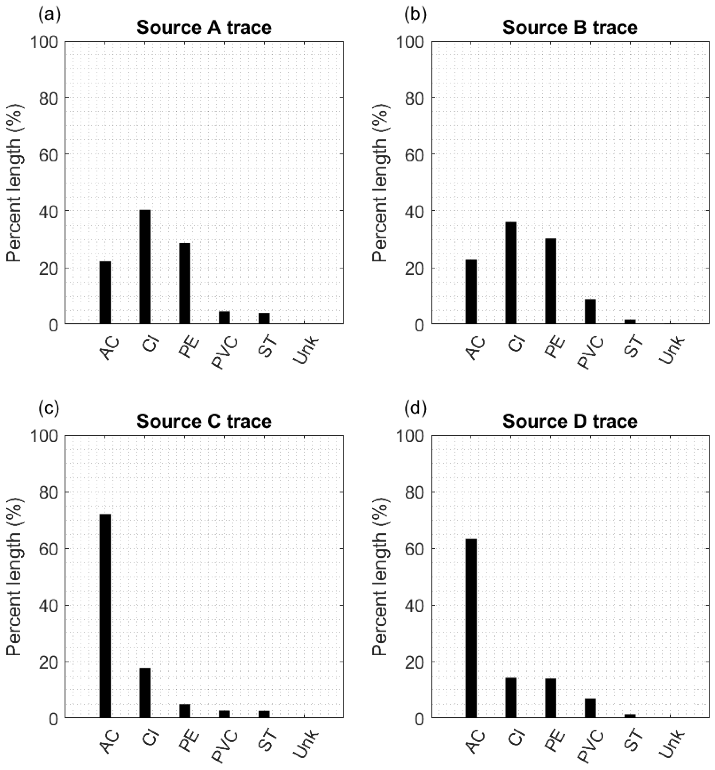
2.1.1. Step 1. Trace Analysis

The first step of the proposed method includes trace analysis, i.e., the modeling of the movement of a non-reactive tracer material through the network over time. This kind of analysis allows one to identify which portions of the network are supplied by each source $j$ ($j=1,\dots ,n_S$). From an operational standpoint, trace analysis is conducted by performing an extended-period simulation over a period allowing model warm-up [27] and by considering the resulting average water velocities in pipelines in relation to the end of the period. In greater detail, for each node $k$ of the WDN ($k=1,\dots ,n_N$), trace analysis is carried out by evaluating the fractions (i.e., percent value) of water supplied to the node by each source $j$ by means of the EPANET 2.2 water quality simulator. This information can be summarized in a matrix $T$ with $n_N$ rows and $n_S$ columns, in which the generic element $T_{k,j}$ is the trace of source $j$ at node $k$. Therefore, nodes (i.e., rows of matrix $T$) that are supplied by a single source $s$ present a value of 100 (%) in the $j$-th element of the row, i.e., $T_{k,j}=100$. Conversely, nodes supplied by more than one source present positive values in matrix $T$columns related to all sources supplying them. In any case, the sum of all percent values along every row of matrix $T$ must be equal to 100% to ensure nodal flow balance, i.e., ${{\displaystyle \sum }}_{j=1}^{n_S}{T}_{k,j}=100$. It is worth noting that the methodology here proposed is valid even if the overall WDN is supplied by a single source (i.e., $n_S=1$), being, in this case, matrix $T$ equal to a column vector including 100 in each element (i.e., $T_{k,1}=100 \forall k=1,\dots ,n_N$).

2.1.2. Step 2. Assignment of Weights to Pipes Based on Trace Analysis

The second step of the method is aimed at assigning a set of $n_S$ weights to each link of the WDN based on the results of trace analysis included in matrix $T$. In greater detail, each link $i$ ($i=1,\dots ,n_L$) is considered in turn. Then, for each source $j$, a weight $w_{i,j}$ describing the source contribution to the selected link is evaluated based on the average flow rate and considering the pipe upstream node $u_i$ (i.e., pipe starting node according to the direction of the average flow rate) as shown in Equation (1).

$$w_{i,j}=T_{u_i,j}$$

(1)

From an operational standpoint, all values $w_{i,j}$ are finally included in the matrix of link weights, namely $W$ [$n_L\times n_S$]. It is worth noting that, at the end of step 2, each link of the WDN (i.e., each row of matrix $W$) is described by $n_S$ weights representing the contribution of each source to selected link. In the case of a pipeline $i$ lying in a WDN area unaffected by water mixing (i.e., supplied by a single source $j$), only the weight $w_{i,j}$related to that source would be equal to 100 (all other weights being equal to zero), whereas pipelines in areas affected by water mixing result in several positive weights, the sum of which is equal to 100.

2.1.3. Step 3. Identification of Overall Reaction Rates

In general, the distribution of RCC varies over time and across the network due to a series of physical and chemical decay reactions that progressively consume disinfectants. Decay is mainly due to the reactions that take place in the bulk volume and at the pipe wall [23]. On the one hand, bulk decay depends on water characteristics, e.g., the concentration of natural organic and inorganic matter, water temperature, and disinfectant concentration. On the other hand, pipe wall decay depends on pipe age, pipe material, and the presence of corrosion and/or biofilm [28].

Under the assumption of a constant pipe section, chlorine decay can be modeled as a first-order reaction as shown in Equation (2) [29]:

$$\frac{\partial C\left(t\right)}{\partial t}=-\left(k_b+\frac{k_w}{r_h}\right)C\left(t\right)$$

(2)

where $C\left(t\right)$ is chlorine concentration (mass/volume) over time $t$, $k_b$ is a decay coefficient related to bulk chlorine degradation (1/time), $k_w$ is a decay coefficient related to pipe wall degradation (length/time), and $r_h$ is pipe hydraulic radius (length). Specifically, EPANET’s water quality simulator introduced by [30] is here assumed to track the decay of chlorine by reaction as it travels through a distribution system based on Equation (2).

Coefficients $k_b$ and $k_w$ can be complicated to assess given their dependence on several aspects but also in the face of the fact that, with specific reference to $k_b$, models in the literature do not generally provide a good fit with observed data [23]. In light of the difficulties related to the accurate estimation of individual $k_b$ and $k_w$ decay contributions [25]—and to reduce the uncertainty related to the number of variables—a formulation based on an overall rate coefficient $K$ (1/time) (hereinafter referred to as overall reaction rates) is assumed and, thus, Equation (2) is simplified as shown in Equation (3):

$$\frac{\partial C\left(t\right)}{\partial t}=-KC\left(t\right)$$

(3)

The third step of the methodology consists in the identification of the overall reaction rate values $K_j$ for each source $j$, i.e., the calibration of the WDN chlorine decay model based on a single water quality parameter for each source.

From an operational standpoint, an automated, interval-number-based method is applied to investigate the range of parameter $K_j$ values ($j=1,\dots n_S$). The method relies on the use of the EPANET–MATLAB^® toolkit (i.e., the combination of EPANET 2.2 software for hydraulic and water quality modeling and MATLAB^® R2019a programming software). Overall reaction rates $K_j$ are considered as interval numbers [31,32]. Specifically, parameters $K_j$ are associated to ranges ${\left[K_{min};K_{max}\right]}_j$ so that all the RCC ranges ${\left[C_{min}^{sim};C_{max}^{sim}\right]}_p$ resulting from hydraulic simulation for each sampling point $p$include their related observed values $C_p^{obs}$. The method is structured as detailed below:

(i)

An initial-attempt interval ${\left[K_{min},K_{max}\right]}_j^0$ is defined for the overall reaction rates $K_j$ related to each source $j$;

(ii)

The lower limit $K_{min,j}^0$ of all the $j$-interval numbers is first considered. A reaction parameter $k_{min,i}$ is assigned to each link $i$ of the WDN, in turn, based on the weighted average of the overall reaction rates $K_{min,j}^0$as shown in Equation (4):

$$k_{min,i}={\displaystyle \sum }_{j=1}^{n_S}{w}_{i,j}·K_{min,j}^0$$

(4)

(iii)

Water quality simulation is performed and the resulting RCC values at each sampling point $p$ are considered. In greater detail, given the nature of the chlorine decay reaction, the imposition of the lower limits of the overall reaction rates values $K_{min,j}^0$ would result in the highest simulated RCC values, i.e., $C_{max,p}^{sim}$;

(iv)

The upper limit $K_{max,j}^0$ of all the $j$-interval numbers is then considered. A reaction parameter $k_{max,i}$ is assigned to all the $i$-links of the WDN, in turn, based on the weighted average of the overall reaction rates $K_{max,j}^0$as shown in Equation (5):

$$k_{max,i}={\displaystyle \sum }_{j=1}^{n_S}{w}_{i,j}·K_{max,j}^0$$

(5)

(v)

Water quality simulation is performed and the resulting RCC values at each sampling point $p$ are considered. In this case, the imposition of the upper limits of the overall reaction rates $K_{max,j}^0$ would result in the lowest simulated RCC values, i.e., $C_{min,p}^{sim}$;

(vi)

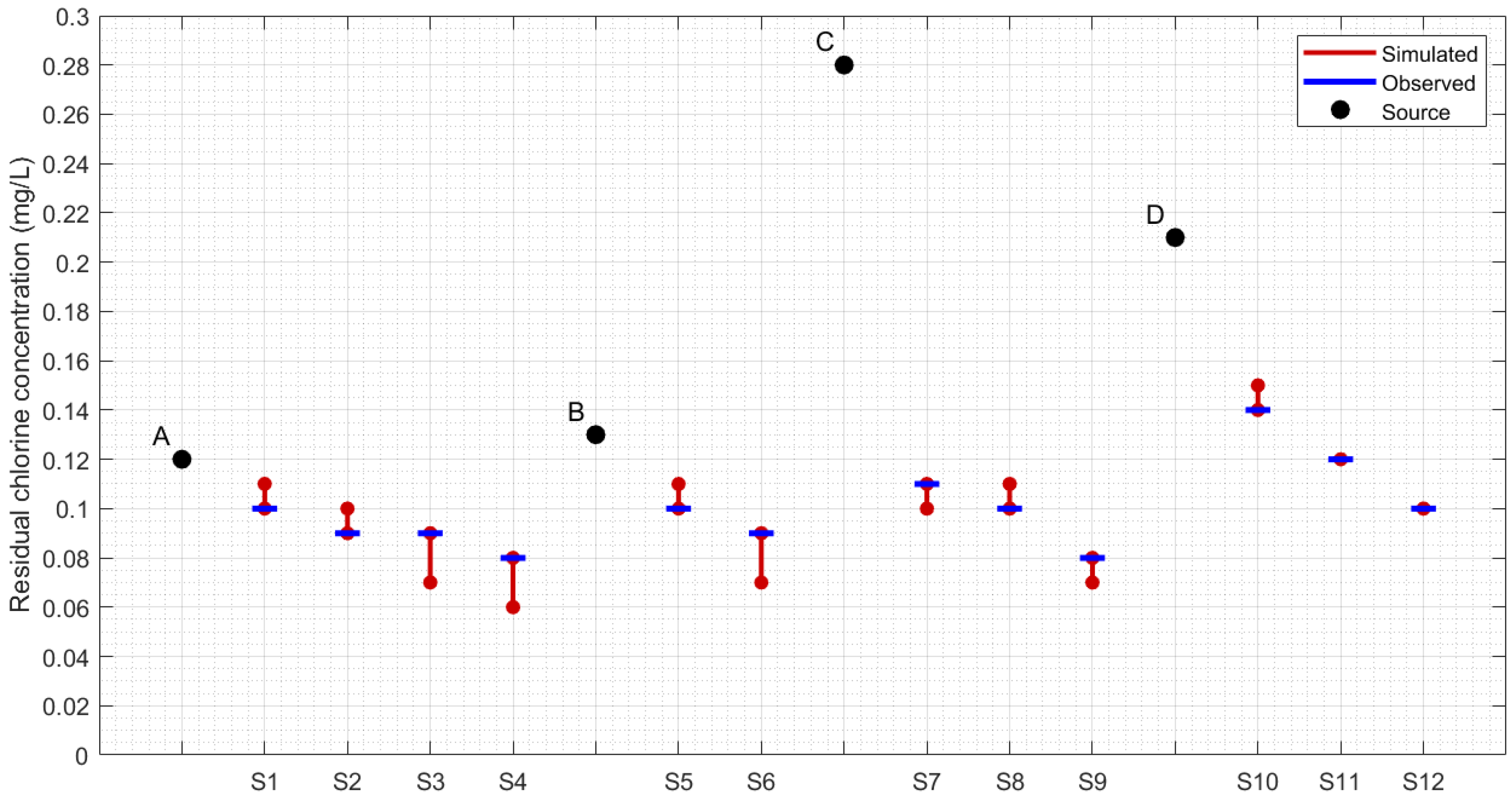
The observed RCC values $C_p^{obs}$ are compared against the respective RCC ranges ${\left[C_{min}^{sim};C_{max}^{sim}\right]}_p$ obtained through hydraulic simulations, i.e., interval numbers $C_p^{sim}$. In the event that all the observed values $C_p^{obs}$ fall within their respective simulated ranges (i.e., $C_p^{obs}\in C_p^{sim}$), the overall process (i.e., phases i–v) is repeated by reducing the amplitude of each interval number $K_j$. The process stops when the narrowest interval numbers $K_j$ satisfying the above conditions are found. In other words, an interval ${\left[K_{min},K_{max}\right]}_j$ describing the overall reaction rate for each area $j$ supplied by a source is obtained at the end of phase vi.

The results obtained can finally be interpreted based on the mean and amplitude of the interval numbers $K_j$ related to a WDN’s overall reaction rate.

2.2. Case Study

The methodology presented in Section 2.1 is tested on a real case of a WDN, i.e., the network supplying the Piovese region in northern Italy (Figure 2a). The Piovese WDN, managed by AcegasApsAmga S.p.A, is characterized by a length of 810 km but despite its considerable length, it supplies a rather limited number of users (around 30,000, i.e., an average of less than 40 users/km). This is primarily related to the fact that the Piovese region is a predominantly rural area, characterized by a low population density. Pipe characteristics in the network are heterogeneous. Pipe ages range from over 70 years (i.e., pipes laid in the 1950s) to less than 10 years (i.e., pipes laid in the 2020s), with an average age of about 40 years. Concerning the materials, WDN pipes are mainly made of asbestos cement (AC) (292 km, i.e., 36%), cast iron (CI) (254 km, i.e., 31%), polyethylene (PE) (192 km, i.e., 24%), polyvinyl chloride (PVC) (51 km, i.e., 6%), and steel (ST) (21 km, i.e., 3%).

The Piovese WDN is supplied by four sources, hereinafter indicated as sources A, B, C, and D and represented as black dots in Figure 2b. From an operational standpoint, Source A and Source B supply the northern part of the WDN whereas Source C and Source D supply the southern part of the system. As far as water quality is concerned, it is worth noting that the four sources supplying the WDN show different characteristics, as indicated in

Table 1. Water characteristics for the four sources.

Source	Avg. Inflow (L/s)	Water	Chlorine Concentration (mg/L)
A	160	underground aquifer	0.12
B	70	mixed water a	0.13
C	20	surface water	0.28
D	60	mixed water b	0.21

Notes: ^a Source B includes 70% of re-chlorinated water from sources C and D and a residual 30% of water from a nearby WDN; ^b Source D includes 90% of surface water (the same as source C) and a residual 10% of water from a nearby WDN.

. On the one hand, the northern WDN part is primarily supplied by water withdrawn from underground aquifers (Source A, providing about 160 L/s) but also by mixed water (Source B, providing about 70 L/s). On the other hand, the southern WDN part is mainly served by surface water withdrawn from the Adige River (making up 100% of water from Source C and 90% of source D, providing about 80 L/s overall). At each source, the water is chlorinated, ensuring a constant concentration at each inlet point, even though the concentration set points change from source to source (see Table 1).

From an operational standpoint, RCC is monitored by the AcegasApsAmga S.p.A. water utility through a system of $n_P=12$ points distributed throughout the WDN (represented as red dots in Figure 2). The location of sampling points was preliminary defined by the water utility in order to observe RCC in as many areas as possible. Sampling is fully automated and relies on a smart-metering systems including RCC devices (with an accuracy of 0.01 mg/L) paired with data loggers and transmitters collecting and sending the data with a time resolution of 1 h.

Overall, the hydraulic model of the Piovese WDN—previously calibrated based on hydraulic data (i.e., pressure, flow rate, water level) observed over a period of ten days in year 2021—is made available by the AcegasApsAmga S.p.A. water utility, in order to evaluate the effectiveness of the proposed methodology. Specifically, the model includes $n_N$ = 10,605 nodes and $n_L$ = 10,916 links. Besides the hydraulic model, RCC data collected at each sampling point $p$ ($p=1,\dots ,n_P$) over the whole year of 2021 are provided. It is worth noting that, due to the characteristics of water chlorination at sources A–D (aimed at ensuring a constant chlorine concentration at their outflow) with the consequent reduced variations in the daily trend of RCC at different sampling points, all subsequent analyses are carried out by considering yearly average RCC values.

3. Results and Discussion

The application of the proposed method for chlorine decay modeling to the Piovese WDN case study is discussed in the following.

The results of step 1 of the method (trace analysis) are shown in Figure 3, where panels refer to the four sources in relation to which trace analysis is conducted (Sources A–D). Specifically, the trace values reported in the figure are averaged across the last day of hydraulic simulation; different dot colors relate to different trace levels at the WDN nodes, ranging from light yellow in the case of a trace > 10% (i.e., source supplying the node considered in a limited manner) to dark red in the case of a trace > 90% (i.e., source supplying the node considered almost entirely). Figure 3 reveals that, due to its looped layout, the WDN considered includes areas supplied by mixing waters from different sources. This occurs both in the northern part of the network (where waters from Source A and Source B are mixed) and in the southern part (where waters from Source C and Source D are mixed). On the one hand, in the northern part of the network, water from Source A mixes with water from Source B, leading to the appreciable mixing area in the center of the northern part of the WDN. In this mixing area, the sum of traces from Source A and B at single nodes equals 100%. On the other hand, in the southern part of the network, water from Source C mixes with water from Source D, leading to a mixing area which mainly develops along a sub-horizontal main pipe, where the sum of traces from Source C and D at single nodes equals 100%. Overall, the multi-source nature of the WDN and the consequent presence of many areas where water mixing occurs represent a point of complexity and make the case study here considered more challenging as opposed to most networks considered in similar studies available in the literature, featuring a simplified layout and typically supplied by a single source.

The results of trace analysis—i.e., the identification of the trace of each of the $n_S=4$ sources to all $n_N$ network nodes—allow us to obtain a set of $n_S$ weights to assign to each of the $n_L$ network links and, therefore, to apply the interval-number-based method defined in Section 2. Specifically, $n_S=4$ interval numbers $K_j$ (one per source, i.e., being $j=\left\{A,B,C,D\right\}$) are defined, and the automated, iterative approach based on the results of hydraulic and water quality simulation presented in Section 2.1.3 is considered. From an operational standpoint, a sufficiently wide first-attempt interval number $K_j^0={\left[K_{min}^0;K_{max}^0\right]}_j=\left[0;100\right] {\mathrm{days}}^{-1}$ is assigned to each source, in order to make the solution space broad and able to cover many scenarios of chlorine decay in the WDN considered. In fact, it is worth noting that an overall reaction rate equal to 0 ${\mathrm{days}}^{-1}$($K_{min}^0$) would result in no decay, i.e., non-reactive tracer, whereas an overall reaction rate equal to 100 ${\mathrm{days}}^{-1}$($K_{max}^0$) would result in a considerably rapid decay, so that the RCC would tend to zero in a very limited time. The $n_S$ interval numbers $K_j$ are then iteratively reduced as detailed in phases i-v, by considering a reduction step (i.e., increase in the lower limit $K_{min,j}$ and decrease in the upper limit $K_{max,j}$ comparable to the accuracy of RCC meters installed in the WDN (0.01 mg/L)) and performing hydraulic simulation at each step. For each of these scenarios, i.e., given each set of extreme values of the interval numbers $K_j$, hydraulic simulation across a period of 10 days is conducted, but only the average values across the last day of simulation are considered. This is due to the need for a model warm-up in relation to RCC values, because the initial RCC valued are unknown for almost all network nodes (except for those including a sampling point). In addition, a simulation time-step of 5 min is considered, in order to avoid model inaccuracies and accommodate the short times of travel that can occur within pipes [30].

The automated, iterative process leads to the obtainment of the interval number values $K_j$ for each source as shown in

Table 2. Overall reaction rates (interval numbers $K_j$) obtained.

Source	$\mathbf{Minimum} \mathbf{Reaction} \mathbf{Rate} {\mathit{K}}_{\mathit{m}\mathit{i}\mathit{n}}$ (1/days)	$\mathbf{Maximum} \mathbf{Reaction} \mathbf{Rate} {\mathit{K}}_{\mathit{m}\mathit{a}\mathit{x}}$ (1/days)
A	0.70	1.10
B	0.40	0.50
C	0.95	1.05
D	0.95	1.05

. The application, in turn, of (the weighted average of) these values to all network links leads to the simulated RCC values shown in Figure 4, where the interval numbers $C_p^{sim}={\left[C_{min}^{sim};C_{max}^{sim}\right]}_p$ related to the simulated RCC at each sampling point $p$ against the related average values observed in the field $C_p^{obs}$ are also shown. Specifically, black dots refer to sources, the RCC values at which are those indicated in Table 1. As far as the simulated RCC interval numbers $C_p^{sim}$ are concerned, Figure 4 reveals that these intervals include all the average observed RCC values $C_p^{obs}$, meaning that the overall reaction rates $K_j$ identified by the method effectively reflect the chlorine decay phenomena despite the complex multiple-source WDN here considered. Moreover, the amplitude of the simulated RCCs $C_p^{sim}$ is generally limited to 0.01 mg/L (or less) for all sampling points, except in three cases (points S3, S4, and S6) in relation to which it increases up to 0.02 mg/L. However, this maximum amplitude is in line with the accuracy of the instrument installed by the water utility for RCC monitoring, demonstrating that the method is effective without specific information on pipe features in the WDN concerned (affecting wall decay) nor details about the characteristics of the water supplied by each source (affecting bulk decay). Overall, the results obtained confirm the method’s capability to effectively describe chlorine decay reactions. The approach here considered, including the assignment of a weighted average of a few, global parameters to all network links based on the results of a preliminary trace analysis, makes the method a valid tool for a pragmatic water quality modeling with no need for expensive and resource-consuming field and laboratory tests aimed at estimating bulk and wall chlorine reaction rates.

In light of the results obtained, it is also possible to make considerations about the average value and the amplitude of the $n_S$ interval numbers $K_j$ describing the overall reaction rates, based on which a weighted rate has been assigned to each WDN pipe. On the one hand, as shown in Equation (3), the average value of each interval number $K_j$ can be assumed representative of the average decay rate, which is primarily dependent on the tendency of the disinfectant to react with the substances available in the water bulk or on pipe wall. On the other hand, the amplitude of a given interval number $K_j$ can be related to a variety of pipe characteristics affecting chlorine decay (i.e., material and age) which may produce local differences in terms of overall reaction rate. Based on the overall reaction rates shown in Table 2, it emerges that: (1) the interval number related to Source A has greater amplitude and a higher average value compared to Source B, suggesting differences in terms of type of water between the two sources (Table 1) and/or pipe characteristics; (2) the interval numbers related to Source C and Source D have small amplitude and a high average value, mainly suggesting a higher reaction rate as opposed to sources A and B. Also, the same values obtained for sources C and D highlight a similar behavior in terms of chlorine decay, likely due to similar types of water (Table 1) along with a possible homogeneity in pipe characteristics.

For a better interpretation of the above considerations, the age and material of all pipes in the case study considered are investigated based on the information made available by the water utility managing the WDN. In greater detail, each pipe $i$ is assigned to the source related to the highest trace, i.e., for source $j$, the weight $w_{i,j}$ is the greatest. Pipe age and material distributions in relation to the percent length of all pipes assigned to each source are shown in Figure 5 (age) and Figure 6 (material). In particular, it emerges that the areas mainly supplied by Source A and Source B tend to show a variety in pipe ages and materials (with no predominance of a given age or material class), whereas those mainly supplied by Source C and Source D are primarily characterized by steel pipes, whose ages mainly fall in the range 1970–1990. On the one hand, considering the northern part of the WDN, the heterogeneity in pipe ages and materials in area mainly supplied by Source A is believed to motivate the spread in the overall reaction rate values (i.e., interval number $K_A$) associated with this source. In other words, as previously discussed, a variety of ages and materials are likely to result in a large amplitude of the range of the overall reaction rate, highlighting different reaction rates across space. On the other hand, as far as the southern part of the system is concerned, the reduced amplitudes of interval numbers $K_C$ and $K_D$ are likely to be related to the greater homogeneity in network characteristics, resulting in similar WDN behaviours across different areas. Therefore, the results obtained from the analysis of pipe age and material distributions further support the results obtained by applying the water quality modeling method here considered, based on the identification of global decay parameters (i.e., overall reaction rates $K_j$).

4. Study Limitations and Requirements

Despite the promising results achieved, some limitations can be identified in the current study. The limitations of the approach proposed are briefly reported in this section along with operational requirements:

• Although (i) the main aim of the study here proposed is to provide a pragmatic tool for water quality calibration and (ii) the calibration approach is based on the use of RCC data observed in the field over a reliable period (i.e., in relation to a yearly time window in the case of the Piovese WDN), the unavailability of additional RCC data observed over different periods did not make it possible to further test method performance in subsequent time windows;
• The approach here proposed is based on the use of RCC data collected in the field. Specifically, the installation of at least one RCC sensor per area supplied by a given source is required. In the event that one or many supply areas do not include at least one RCC sensor, model calibration is not possible by means of the interval-number-based method described in this study;
• Although analysis of model sensitivity to overall reaction rate values is not explicitly included in this study, it is worth noting that the interval-number-based nature of the method here presented intrinsically allows one to make considerations about the effects of the overall reaction rate values on RCC spatio–temporal distribution. In greater detail, overall reaction rates $K_j$ are here defined as interval numbers, i.e., ranges, the extreme values of which are adjusted so that all the resulting RCC ranges (obtained from hydraulic simulation) include their related observed values. Overall, the amplitude of these interval numbers reflects the uncertainty related to the respective parameters.

Concerning operational requirements, the proposed method relies on the use of: (i) modeling software, i.e., license-free EPANET 2.2 software, that is specifically used to perform hydraulic simulation and water quality simulations (e.g., trace analysis); (ii) the EPANET–MATLAB^® toolkit, which is used to automatize the method; and (iii) a database obtained through field measurements by exploiting a number of water quality sensors of adequate accuracy (e.g., 0.01 mg/L) and sufficient sampling resolution (e.g., 1 h). Overall, no specific cost implications or requirements are related to the implementation of the approach here proposed, except software licenses and a RCC sensor system (which, however, may be already available in the case of a real WDN).

5. Conclusions

This paper proposes a pragmatic approach for the chlorine decay modeling in multiple-source networks, based on the results of trace analysis and relying on interval numbers. The approach is applied to the case study of the Piovese WDN which is supplied by multiple sources with water of different quality characteristics. Overall, the results obtained highlight that:

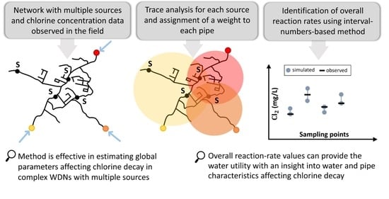
• The developed method—relying on the combination of trace analysis and the use of interval numbers—is effective in estimating the value of global parameters affecting chlorine decay (i.e., overall reaction rates) in complex WDNs with multiple sources, a case which had been explored only in a limited manner in the literature;
• Overall, trace analysis (allowing the identification of those areas where waters with different qualitative characteristics are mixed) is demonstrated to be an effective support tool when modeling chlorine decay in WDNs, overcoming the challenge of the complexity related to the multi-source nature of the WDN. Specifically, the application of the proposed approach can be useful to focus the attention on WDN areas potentially subjected to water-mixing processes, where unexpected general chlorine decay can be observed;
• The use of global water quality parameters (i.e., overall reaction rates) allows one to obtain a chlorine decay model capable of accurately representing the spatio–temporal distribution of RCC throughout a complex WDN without the need of specific information on pipe characteristics (i.e., age and material, affecting wall reactions) or water quality characteristics (affecting bulk reaction) which may be difficult to obtain, as widely demonstrated in the literature;
• Indicators such as amplitude and the average value of the interval numbers describing the overall reaction rates can provide water utilities with an insight into the source and WDN characteristics affecting chlorine decay.

In conclusion, it is believed that the proposed method can easily be transferred to provide water utilities with a water quality model of their network based on which they can carry out strategic evaluations and assessments aimed at an efficient management of systems. Future directions will mainly consist in: (i) further testing method performance based on new RCC data collected in the field and (ii) exploring the effects of the number and the position of RCC sensors on method effectiveness.

References

- Yimer, T.; Desale, T.; Asmare, M.; Endris, S.; Ali, A.; Metaferia, G. Modeling of Residual Chlorine on Addis Ababa Water Supply Distribution Systems. Water Conserv. Sci. Eng. 2022, 7, 443–452. [Google Scholar] [CrossRef]
- Frankel, M.; Katz, L.E.; Kinney, K.; Werth, C.K.; Zigler, C.; Sela, L. A framework for assessing uncertainty of drinking water quality in distribution networks with application to monochloramine decay. J. Clean. Prod. 2023, 407, 137056. [Google Scholar] [CrossRef]
- Schück, A.; Díaz, S.; Lansey, K. Reducing Water Age in Residential Premise Plumbing Systems. J. Water Resour. Plan. Manag. ASCE 2023, 149, 04023031. [Google Scholar] [CrossRef]
- Udokpoh, U.U.; Ndem, U.A.; Abubakar, Z.S.; Yakasi, A.B.; Saleh, D. Comparative Assessment of Groundwater and Surface Water Quality for Domestic Water Supply in Rural Areas Surrounding Crude Oil Exploration Facilities. J. Environ. Pollut. Hum. Health 2021, 9, 80–90. [Google Scholar] [CrossRef]
- Delgado-Aguiñaga, J.A.; Becerra-López, F.I.; Torres, L.; Besancon, G.; Puig, V.; Jiménez Magaña, M.R. Dynamic model for a water distribution network: Application to leak diagnosis and quality monitoring. IFAC-PapersOnLine 2020, 53, 16679–16684. [Google Scholar] [CrossRef]
- Smeets, P.W.M.H.; Medema, G.J.; van Dijk, J.C. The Dutch secret: How to provide safe drinking water without chlorine in the Netherlands. Drink. Water Eng. Sci. 2009, 2, 1–14. [Google Scholar] [CrossRef]
- Mabrok, M.A.; Saad, A.; Ahmed, T.; Alsayab, H. Modeling and simulations of Water Network Distribution to Assess Water Quality: Kuwait as a case study. Alex. Eng. J. 2022, 61, 11859–11877. [Google Scholar] [CrossRef]
- Quintiliani, C. Water Quality Enhancement in WDNs through Optimal Valves Setting. Ph.D. Thesis, University of Cassino and Southern Lazio, Cassino, Italy, 2017. [Google Scholar]
- Abraham, E.; Blokker, E.J.M.; Stoianov, I. Decreasing the discoloration risk of drinking water distribution systems through optimized topological changes and optimal flow velocity control. J. Water Resour. Plan. Manag. ASCE 2017, 144, 04017093. [Google Scholar] [CrossRef]
- Vreeburg, J.H.G.; Boxall, J.B. Discolouration in potable water distribution systems: A review. Water Res. 2007, 41, 519–529. [Google Scholar] [CrossRef]
- Marsili, V.; Alvisi, S.; Maietta, F.; Capponi, C.; Meniconi, S.; Brunone, B.; Franchini, M. Extending the Application of Connectivity Metrics for Characterizing the Dynamic Behavior of Water Distribution Networks. Water Resour. Res. 2023, 59, e2023WR035031. [Google Scholar] [CrossRef]
- Brentan, B.; Monteiro, L.; Carneiro, J.; Covas, D. Improving water age in distribution systems by optimal valve operation. J. Water Resour. Plan. Manag. ASCE 2021, 147, 04021046. [Google Scholar] [CrossRef]
- Quintiliani, C.; Marquez-Calvo, O.; Alfonso, L.; Di Cristo, C.; Leopardi, A.; Solomatine, D.P.; de Marinis, G. Multiobjective valve management optimization formulations for water quality enhancement in water distribution networks. J. Water Resour. Plan. Manag. ASCE 2019, 145, 04019061. [Google Scholar] [CrossRef]
- Garcia, D.; Puig, V.; Quevedo, J. Prognosis of Water Quality Sensors Using Advanced Data Analytics: Application to the Barcelona Drinking Water Network. Sensors 2020, 20, 1342. [Google Scholar] [CrossRef] [PubMed]
- Lu, H.; Ding, A.; Zheng, Y.; Jiang, J.; Zhang, J.; Zhang, Z.; Xu, P.; Zhao, X.; Quan, F.; Gao, C.; et al. Securing drinking water supply in smart cities: An early warning system based on online sensor network and machine learning. AQUA Water Infrastruct. Ecosyst. Soc. 2023, 72, 721. [Google Scholar] [CrossRef]
- World Health Organization. Guidelines for Drinking Water Quality; World Health Organization: Geneva, Switzerland, 2017. [Google Scholar]
- Pérez, R.; Martínez-Torrents, A.; Martínez, M.; Grau, S.; Vinardell, L.; Tomàs, R.; Martínez-Lladó, X.; Jubany, I. Chlorine Concentration Modelling and Supervision in Water Distribution Systems. Sensors 2022, 22, 5578. [Google Scholar] [CrossRef] [PubMed]
- Pecci, F.; Stoianov, I.; Ostfeld, A. Convex Heuristics for Optimal Placement and Operation of Valves and Chlorine Boosters in Water Networks. J. Water Resour. Plan. Manag. 2021, 148, 04021098. [Google Scholar] [CrossRef]
- Moeini, M.; Sela, L.; Taha, A.F.; Abokifa, A.A. Bayesian Optimization of Booster Disinfection Scheduling in Water Distribution Networks. Water Res. 2023, 242, 120117. [Google Scholar] [CrossRef]
- Alsaydalani, M.O.A. Simulation of Pressure Head and Chlorine Decay in a Water Distribution Network: A Case Study. Open Civ. Eng. J. 2019, 13, 58–68. [Google Scholar] [CrossRef]
- Bouzid, S.; Ramdani, M.; Chenikher, S. Quality Fuzzy Predictive Control of Water in Drinking Water Systems. Autom. Control. Comput. Sci. 2019, 53, 492–501. [Google Scholar] [CrossRef]
- Fisher, I.; Kastl, G.; Sathasivan, A. New model of chlorine-wall reaction for simulating chlorine concentration in drinking water distribution systems. Water Res. 2017, 125, 427–437. [Google Scholar] [CrossRef]
- Maleki, M.; Ardila, A.; Argaud, P.-O.; Pelletier, G.; Rodriguez, M. Full-scale determination of pipe wall and bulk chlorine degradation coefficients for different pipe categories. Water Supply 2023, 23, 657–670. [Google Scholar] [CrossRef]
- Minaee, R.P.; Mokhtari, M.; Moghaddam, A.; Ebrahimi, A.A.; Askarishahi, M.; Afsharnia, M. Wall Decay Coefficient Estimation in a Real-Life Drinking Water Distribution Network. Water Resour. Manag. 2019, 33, 1557–1569. [Google Scholar] [CrossRef]
- Al-Araimi, M.M.; Joy, V.M.; Rao, L.S.N.; Feroz, S. Optimization and Assessment of Residual Chlorine using Response Surface Methodology (RSM) and Artificial Neural Network (ANN) Modeling. Int. J. Recent Technol. Eng. 2019, 8, 258–263. [Google Scholar] [CrossRef]
- Moghaddam, A.; Mokhtari, M.; Afsharnia, M.; Minaee, R.P. Simultaneous Hydraulic and Quality Model Calibration of a Real-World Water Distribution Network. J. Water Resour. Plan. Manag. 2020, 146, 06020007. [Google Scholar] [CrossRef]
- Medina, Y.; Muñoz, E. Analysis of the Relative Importance of Model Parameters in Watersheds with Different Hydrological Regimes. Water 2020, 12, 2376. [Google Scholar] [CrossRef]
- Monteiro, L.; Carneiro, J.; Covas, D.I.C. Modelling chlorine wall decay in a full-scale water supply system. Urban Water J. 2020, 17, 754–762. [Google Scholar] [CrossRef]
- Digiano, F.A.; Zhang, W. Pipe section reactor to evaluate chlorine-wall reaction. J. Am. Water Work. Assoc. 2005, 97, 74–85. [Google Scholar] [CrossRef]
- Rossman, L.A.; Woo, H.; Tryby, M.; Shang, F.; Janke, R.; Haxton, T. EPANET 2.2 User Manual; Water Infrastructure DivisionCenter for Environmental Solutions and Emergency Response, U.S. Environmental Protection Agency: Cincinnati, OH 45268, USA, 2020. [Google Scholar]
- Alvisi, S.; Franchini, M. Pipe roughness calibration in water distribution systems using grey numbers. J. Hydroinformatics 2010, 12, 424–445. [Google Scholar] [CrossRef]
- Marín, L.G.; Cruz, N.; Sáez, D.; Sumner, M.; Núñez, A. Prediction interval methodology based on fuzzy numbers and its extension to fuzzy systems and neural networks. Expert Syst. Appl. 2019, 119, 128–141. [Google Scholar] [CrossRef]