Spatial Analysis of Aquatic Ecological Health under Future Climate Change Using Extreme Gradient Boosting Tree (XGBoost) and SWAT

Abstract

Climate change not only affects the water resource system but also has a great impact on the aquatic ecosystem, which is complexly linked to various organic and inorganic matter. It is difficult to simulate the current aquatic ecosystem and predict the future system due to the immensity and complexity of aquatic ecosystems; however, a spatial analysis of future aquatic ecological health is necessary if we are to adapt and take action against future climate change. In this study, we evaluated the aquatic ecological health of the Han River basin under the future climate change RCP4.5 and RCP8.5 scenarios using three indices: fish assessment index (FAI), trophic diatom index (TDI), and benthic macroinvertebrate index (BMI). For this, we developed the SWAT-XGBoost linkage algorithm, and the algorithm accuracy for the FAI, TDI, and BMI was 89.3~95.2%. In the case of the FAI and BMI assessment of aquatic ecological health, the upstream Han River was classified as a hot spot. In the case of the TDI, the downstream area of the Han River was classified as a cold spot. However, as the current TDI downstream was classified as grades D and E, continuous management is needed.

1. Introduction

In a river ecosystem, all animals and plants, including fish, need a habitat environment that meets certain conditions for survival and reproduction. However, river ecosystems have been greatly threatened by changes in environmental conditions, such as flow rate and water quality changes. Such environmental changes are closely related to human activities, such as changes in land cover, water use amount, and groundwater level, as well as climate changes. Climate change affects changes in the spatiotemporal distribution characteristics of water resources in the watershed by causing temperature rise, changes in precipitation, and an increase in the occurrence frequency of extreme climates [1,2]. Eventually, the changes mean that hydrologic flow regimes, contaminant and nutrient transport processes, and aquatic ecosystems will change under future climate [3,4]. Accordingly, many researches were performed to assess the impact of climate change on hydrology and water quality in the watershed [5,6,7]. But, there are only a few studies related to changes in river aquatic ecosystems under future climate change. The necessity of studying future aquatic ecosystems still remains a significant field to be covered.

Responses of organisms affected by disturbances, such as stream drying and water temperature changes, in river aquatic ecosystems, provide good data to infer changes in the aquatic environment. In particular, the adherent diatoms in rivers are the primary producers of this type of aquatic ecosystem [8], and they have a short lifespan and short reproductive cycles. Therefore, adherent diatoms are quick to respond to human effects and climate change [9,10]. Due to these characteristics, adherent diatoms, benthic macroinvertebrates, and fishes are used for ecological health assessments in aquatic ecosystems [11,12,13,14]. The fish assessment index (FAI), trophic diatom index (TDI), and benthic macroinvertebrate index (BMI) have usually been used as standard indices in the assessment of aquatic ecological health [13,15,16].

Various mathematical models have been developed to simulate more complex processes in water, soil, crop, and climate systems to determine solutions to environmental issues. However, the models require large quantities of input parameters, such as big data. In contrast to numerical modeling, machine learning needs big input datasets, not parameter sets. Machine learning approaches are another group of models that have been applied during past decades to simulate various hydrological processes, including water dynamics and water quality, and these models have significant prediction accuracy [17].

In order to model rainfall–runoff processes [18,19,20], flood or drought prediction [21,22], sediment and nutrient transport processes [23,24,25], and aquatic ecological status [26,27,28], many kinds of machine learning models, such as artificial neural networks (ANNs), Gaussian mixture models (GMMs), genetic programming (GP), random forests (RFs), and extreme gradient boosting trees (XGBoosts), have been combined with numerical models and have provided satisfactory results. These approaches provide a great prediction capacity and do not require knowledge of various parameters. Machine learning is currently the most popular algorithm that can overcome the disadvantages of other modeling approaches. Coupling machine learning and numerical modeling in such a way that one complements the weakness of the other could offer a significant improvement in prediction accuracy while also maintaining a reasonable representation of complex processes.

In particular, the XGBoost algorithm has been widely used in machine learning for hydrological and environmental problems. XGBoost algorithm was used to simulate river streamflow using meteorological data [29]. Also, it was applied to forecasted streamflow at ungauged sites undergoing drought [30]. Compared with the general linear models built with traditional approaches, most results have shown that the XGBoost model achieves better time-series results in the field of water resources and environmental sciences.

The main objective of this study was to predict spatiotemporal ecological health indices (EHIs) and analyze the change in future EHIs under representative concentration pathway (RCP) scenarios (RCP4.5 and 8.5) in the river system of the Han River watershed (34,148 km²) in South Korea using the XGBoost algorithm with EHI monitoring data and the Soil and Water Assessment Tool (SWAT) model output. Ultimately, this study demonstrates the good performance of a coupled machine learning and numerical modeling (SWAT) method; specifically, the coupling was completed in such a way that one complements the weakness of the other to offer a significant improvement in prediction accuracy for complex environmental processes.

2. Materials and Methods

2.1. Study Area and Data Collection

2.1.1. Study Area

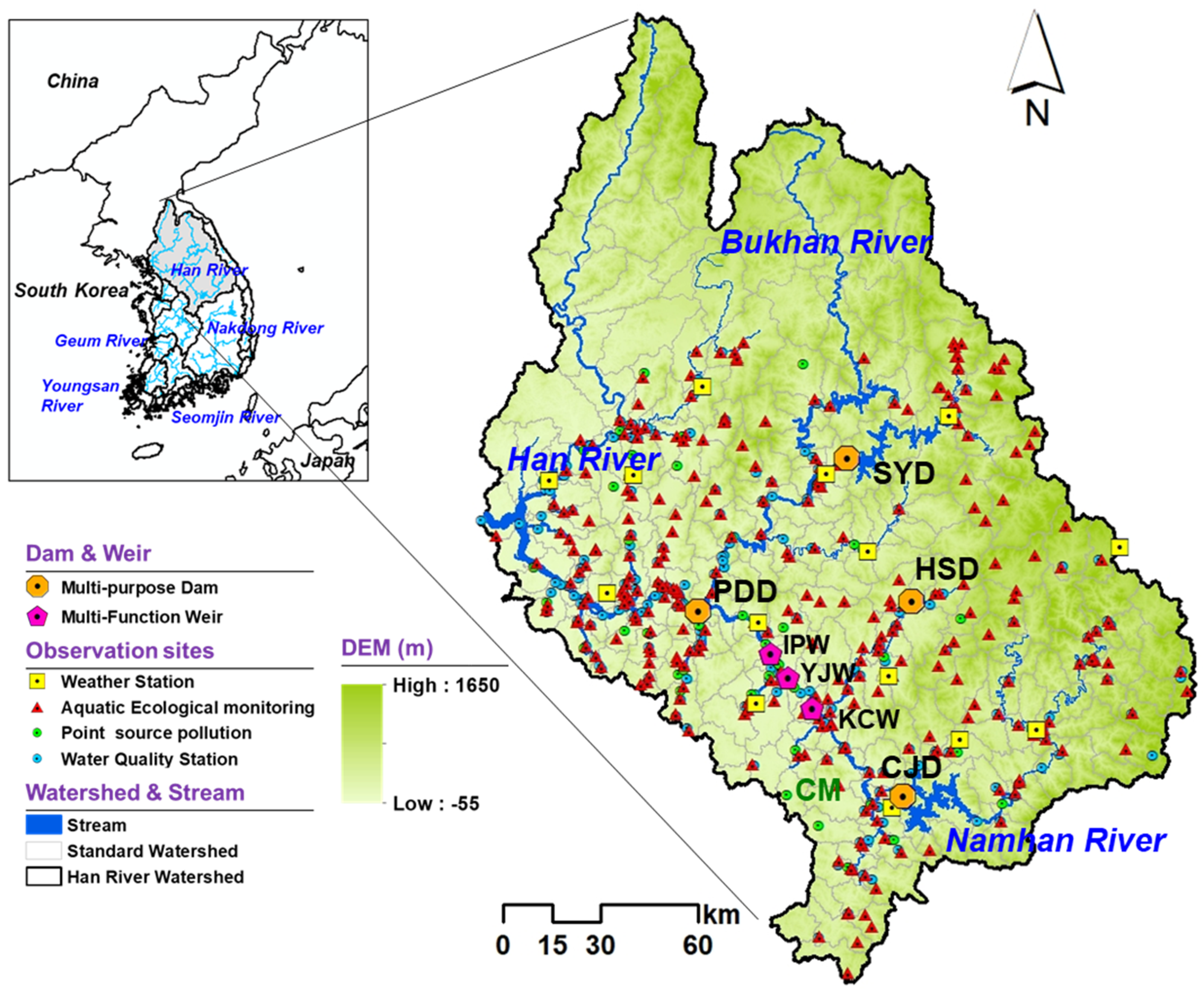
The study area, the Han River watershed (34,148 km²), is located in the northern part of South Korea within the latitude–longitude range of 36.03–38.55° N and 126.24–129.02° E (Figure 1). The watershed is divided into 237 sub-watersheds, called the standard watershed of Korea hydrologic unit map, and among them, 57 sub-watersheds located in the northern part have no available data. The main river of the watershed consists of two streams, the Bukhan River (10,652 km²) and Namhan River (12,514 km²), which merge at the Paldang dam (PDD) and then flow to the outlet of the watershed through the metropolitan city of Seoul.

The watershed has a number of hydraulic structures, such as dams and weirs, controlling the flow to preserve the environment of the watershed and to decrease the damage of floods and droughts. The multipurpose dams of SYD, HSD, and CJD have storage capacities of 2.9 billion m³, 87 million m³, and 2.8 billion m³, respectively. Additionally, the multifunctional weirs of KCW, YJW, and IPW were constructed in 2012 and have total storage capacities of 11 million m³, 13 million m³, and 17 million m³, respectively. The flow through these dams and weirs is controlled by one hydroelectric dam (PDD) with a storage capacity of 244 million m³. The PDD is a major source of water use for downstream metropolitan cities, including Seoul, and supplies approximately 2.6 million m³ of water per day.

The average annual precipitation is 1254 mm, and the average temperature is 11.5 °C based on data that have been collected from 14 weather stations around the basin for 32 years (1984–2015). More than two-thirds of the annual precipitation is concentrated in the summer season (June to September), and precipitation is greater in the eastern area with forests and high elevations. This study used 313 aquatic ecological monitoring sites, 47 point-source pollution sites, and 232 water quality observation sites.

Table 1. List of input data sources.

Input Data	Number of Sites	Time Scale	Period	Provider
Weather	14	Daily	1984~2015	Meteorological Administration
Aquatic Ecological health	313	Semi-annual	2008~2015	Ministry of Environment
Point source	47	Yearly	2008~2015	Ministry of Environment
Water Quality	232	Monthly	2008~2015	Ministry of Environment

provides information on data sources, data collection period, and time scale. These sites are generally more distributed in the downstream region of the watershed, which has suffered from water quality issues due to urbanization.

2.1.2. Ecological Health Monitoring Data

South Korea has developed and operated a nationwide multi-biological monitoring program, the National Aquatic Ecological Monitoring Program (NAEMP), to assess the comprehensive health of rivers using biological criteria by the Ministry of Environment and the National Institute of Environmental Research (NIER) since 2008. The NAEMP is conducted two periods per year, including spring (April to June) and fall (August to October), at 1200 sites covering the whole country; these periods represent the times before and after the summer monsoon, during which there is heavily concentrated precipitation [31]. The monitoring results of NAEMP are used to calculate the score and grade of three aquatic organism indices, such as the TDI, BMI, and FAI [32]. In this study, we considered the three aquatic organism indices, the TDI, BMI, and FAI, at 313 monitoring sites in the Han River watershed.

The TDI is calculated using the abundance of the trophic diatom species in the sample ($A_j$), the species’ pollution sensitivity (1 ≤ $S_j$ ≤ 5), and the indicator value of the species (1 ≤ $V_j$ ≤ 3), as shown in Equation (1). The BMI is calculated using the unit saprobic value of the species ($S_j$), the indicator weight value of the species ($G_j$), and the frequency of the species ($H_j$), as shown in Equation (2). The FAI is calculated using eight metrics (M1 to M8) related to Korean fish assemblages, as shown in Equation (3). Each metric represents the total number of domestic fish species, the number of riffle benthic fish species, the number of intolerant species, the population ratio of tolerant species, the population ratio of species as omnivores, the population ratio of species as domestic insectivores, the total population of sampled domestic species, and the population ratio of abnormalities, respectively. Each of them is scored in three sections (0, 6.25, and 12.5). The equations are as follows:

$$\mathrm{T}\mathrm{D}\mathrm{I}=100-\left[25{\displaystyle \frac{\sum \left(A_j\times S_j\times V_j\right)}{\sum \left(A_j\times V_j\right)}}-25\right]$$

(1)

$$\mathrm{B}\mathrm{M}\mathrm{I}=\left[4-{\displaystyle \frac{\sum \left(S_j\times H_j\times G_j\right)}{\sum \left(H_j\times G_j\right)}}\right]\times 25$$

(2)

$$\mathrm{F}\mathrm{A}\mathrm{I}=M1+M2+M3+M4+M5+M6+M7+M8$$

(3)

The ecological status of the stream was evaluated by each index and was classified into five grades (A: very good; B: good; C: fair; D: poor; E: very poor) based on the scores of the indices computed using the above equations (

Table 2. Assessment criteria for three indices (TDI, BMI, and FAI).

Index	A (Very Good)	B (Good)	C (Fair)	D (Poor)	E (Very Poor)
TDI	≥90	≥70	≥50	≥30	<30
BMI	≥80	≥65	≥50	≥35	<35
FAI	≥80	≥60	≥40	≥20	<20

).

2.1.3. Climate Change Scenarios

Climate change scenarios provide the predicted information about the future climate, such as precipitation, temperature, humidity, wind speed, and solar radiation. The Intergovernmental Panel on Climate Change (IPCC) suggested four RCP scenarios (RCP2.6, 4.5, 6.0, and 8.5) based on anthropogenic greenhouse gas emissions and mitigation policies [33]. In South Korea, the Korea Meteorological Administration (KMA) provides national standard RCP climate change scenarios with a 12.5 km spatial resolution based on IPCC AR5 using HadGEM3-RA, a regional atmospheric model.

In this study, we selected the RCP4.5 and RCP8.5 scenarios of the KMA. RCP4.5 represents the intermediate mitigation scenario of greenhouse gas reduction, with a stabilized radiation forcing of 4.5 W/m². RCP8.5, on the other hand, is a scenario of very high greenhouse gas emissions (radiative forcing of 8.5 W/m²) that maintains the present emissions level (no reduction). As these two RCP scenarios have different greenhouse gas emissions and mitigation strategies, we analyzed the monthly differences in meteorological characteristics for the projection period divided into the baseline (2005–2015), 2020s (2011–2040), 2050s (2041–2070), and 2080s (2071–2100).

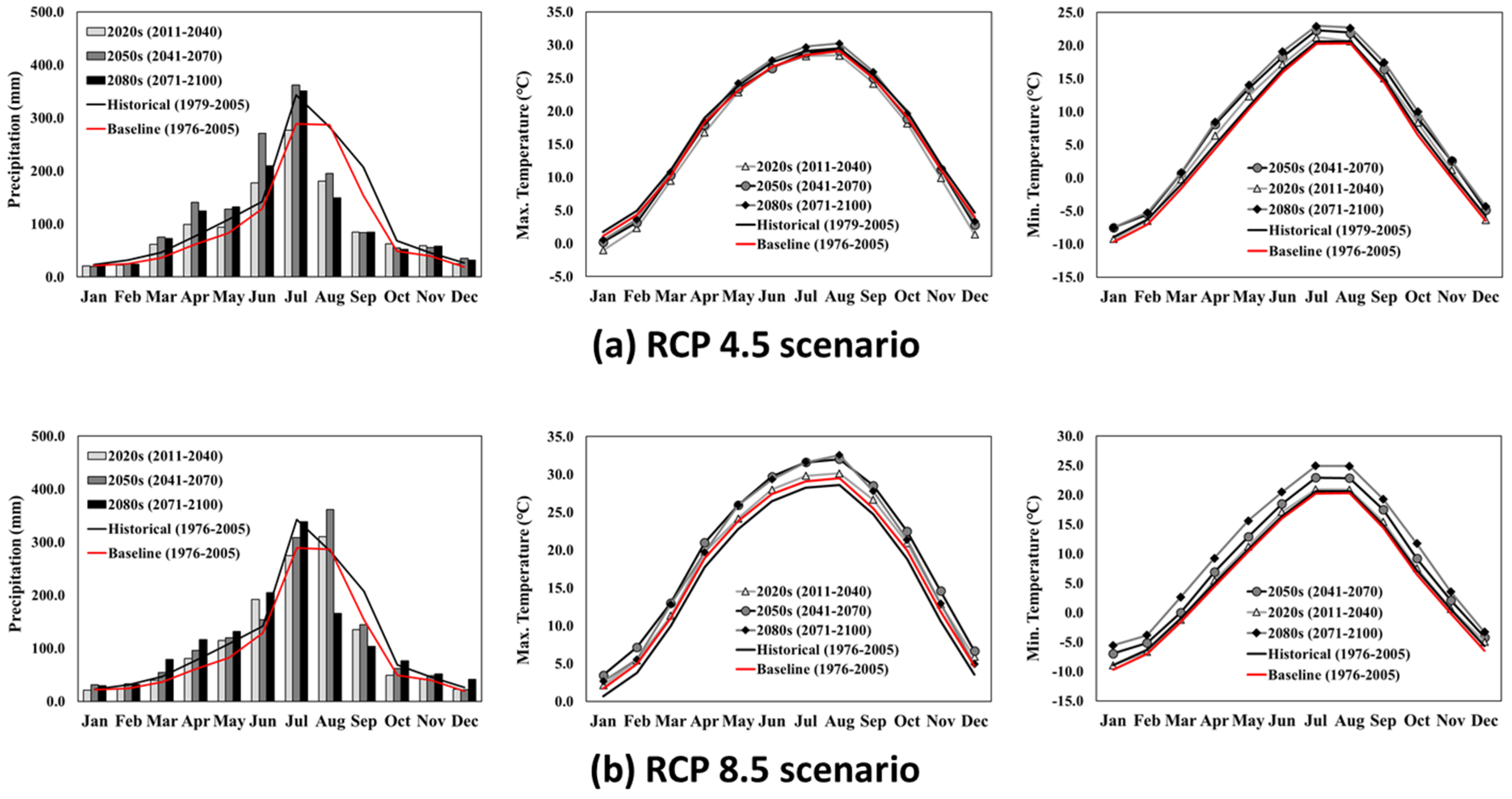
Figure 2 shows the comparisons between climate change RCP scenario data for monthly average precipitation, maximum temperature, minimum temperature, and observation data. In the RCP4.5 scenario, precipitation is expected to increase during April–June and decrease during August–September, and annual precipitation is expected to increase by 253 mm in the 2050s compared to the baseline. Additionally, there is no significant change in the maximum temperature, but there is a 2.8 °C increase in the minimum temperature. Under RCP8.5, the annual precipitation and maximum and minimum temperatures are expected to increase by 115~242 mm, 2.3 °C and 4.3 °C, respectively.

2.2. SWAT

The SWAT is a physical-based, long-term, continuous hydrologic model developed by the USDA-ARS to simulate the impacts of various land cover, soil type, and land management practices [34]. The SWAT simulates hydrological components such as precipitation, surface runoff, lateral flow, baseflow, and water quality components such as sediments, nitrogen, and phosphorus using the concept of hydrologic response units (HRUs). Each HRU, which includes a portion of a sub-watershed with unique land use, management, and soil attributes, is separately calculated and then summed to determine the total yield from the sub-watershed [35].

The hydrologic cycle of SWAT is based on the water balance equation, and the runoff is simulated using a modified SCS-CN method [36]. Erosion and sediment yield are simulated based on the Modified Universal Soil Loss Equation (MUSLE) [37]. Nitrogen and phosphorus are computed in several forms based on the concept of QUAL2E [38], tracking the nutrients dissolved in the stream and adsorbed to sediment. Further detailed processes simulating hydrology, sediment, and nutrient yields are described in the SWAT theoretical documentation [35].

2.3. eXtreme Gradient Boosting Tree (XGBoost)

XGBoost [39] is one of the ensemble algorithms of decision trees to be used for supervised learning problems with training data. The supervised learning models predict target values based on the objective function, which generally consists of training loss term and regularization term. The general objective function, $L$, is expressed as follows:

$$L=\sum _{i}l\left(y_i,{\widehat{y}}_i\right)+\sum _k\mathsf{\Omega }\left(f_t\right)$$

(4)

where $l\left(y_i,{\widehat{y}}_i\right)$ is training loss term, which calculates the difference between the target value $y_i$ and predicted value ${\widehat{y}}_i$, and $\mathsf{\Omega }\left(f\right)$ is regularization term, which is related to model complexity and overfitting.

The objective function of the XGboost algorithm cannot be optimized using traditional optimization methods in

$$L^{\left(t\right)}=\sum _{i=1}^{n}l\left(y_i,{{\widehat{y}}_i}^{\left(t-1\right)}+f_t\left(x_i\right)\right)+\mathsf{\Omega }\left(f_t\right), as {{\widehat{y}}_i}^t={{\widehat{y}}_i}^{\left(t-1\right)}+f_t\left(x_i\right)$$

(5)

$$\begin{gathered} L^{\left(t\right)}=\sum _{i=1}^{n}l\left(y_i,{{\widehat{y}}_i}^{\left(t-1\right)}+g_i{f}_t\left(x_i\right)+{\displaystyle \frac{1}{2}}{h}_i{f_t}^2(x_i)\right)+\mathsf{\Omega }\left(f_t\right)+constant \\ where g_i={\partial }_{{{\widehat{y}}_i}^{\left(t-1\right)}}l\left(y_i{{,\widehat{y}}_i}^{\left(t-1\right)}\right), h_i={{\partial }^2}_{{{\widehat{y}}_i}^{\left(t-1\right)}}l\left(y_i{{,\widehat{y}}_i}^{\left(t-1\right)}\right) \end{gathered}$$

(6)

$${\tilde{L}}^{\left(t\right)}\left(q\right)=-{\displaystyle \frac{1}{2}}\sum _{j=1}^T{\displaystyle \frac{{({\sum }_{i\in I_j}{g}_i)}^2}{{\sum }_{i\in I_j}{h}_i+\lambda }}+\gamma T$$

(7)

The accuracy can be defined as follows:

$$\mathrm{Accuracy} (\mathrm{y}, \overline{y})={\displaystyle \frac{1}{n_{samples}}}{\sum }_{i=0}^{nsamples-1}1(\overline{y}=y)$$

(8)

where i is the number of samples, y is the true value (target value), and $\overline{y}$ is the predicted value.

2.4. Hot Spot Analysis

Hot spot and cold spot analyses were performed to delineate the spatial cluster of the upper primary education level in the Han River basin based on the Getis-Ord Gi* statistic using fixed distance in ArcGIS software (ArcMap 10.3) [40,41]. The Getis-Ord Gi* statistic examines the places or regions where there are statistically significant spatial clumpings of higher magnitudes of a variable, independent of the number of observations. The Getis-Ord Gi* statistic displays z-scores (standard deviations) and p-values (statistical probabilities) that indicate whether the attribute results are statistically clustered, and larger z-scores and lower p-values indicate a spatial clustering of high occurrences of hot spots or a high probability of flooding in the given period. A z-score near zero indicates no apparent spatial clumping for the geographical unit being studied.

2.5. Implementation of the Linkage Technique Combining Machine Learning with SWAT

This study demonstrates a machine-learning approach to predict three aquatic EHIs using calibrated SWAT flow and water quality outputs as inputs to a machine-learning algorithm. The SWAT can simulate all hydrological and water quality variables, which can then be spatially distributed; however, the SWAT cannot determine EHIs from hydrological components. Therefore, this study uses machine learning to make decisions that can determine EHIs, i.e., the observation process for the estimation of EHIs can be replaced with machine learning. Thus, machine learning for the prediction of EHIs is developed using distributed SWAT results, including river flow and water quality. The SWAT results are used as input variables for machine learning. Before developing the model, this study selected independent variables such as flow, total nitrogen (T-N), total phosphorus (T-P), NH₄, NO₃, PO_4, and water temperature (WT). This study selected variables based on whether they were being observed and were components of the SWAT model output. Additionally, the SWAT model results were used as an input variable in spring (April to June) and autumn (August to October) because EHIs have been measured in spring (April to June) and autumn (August to October).

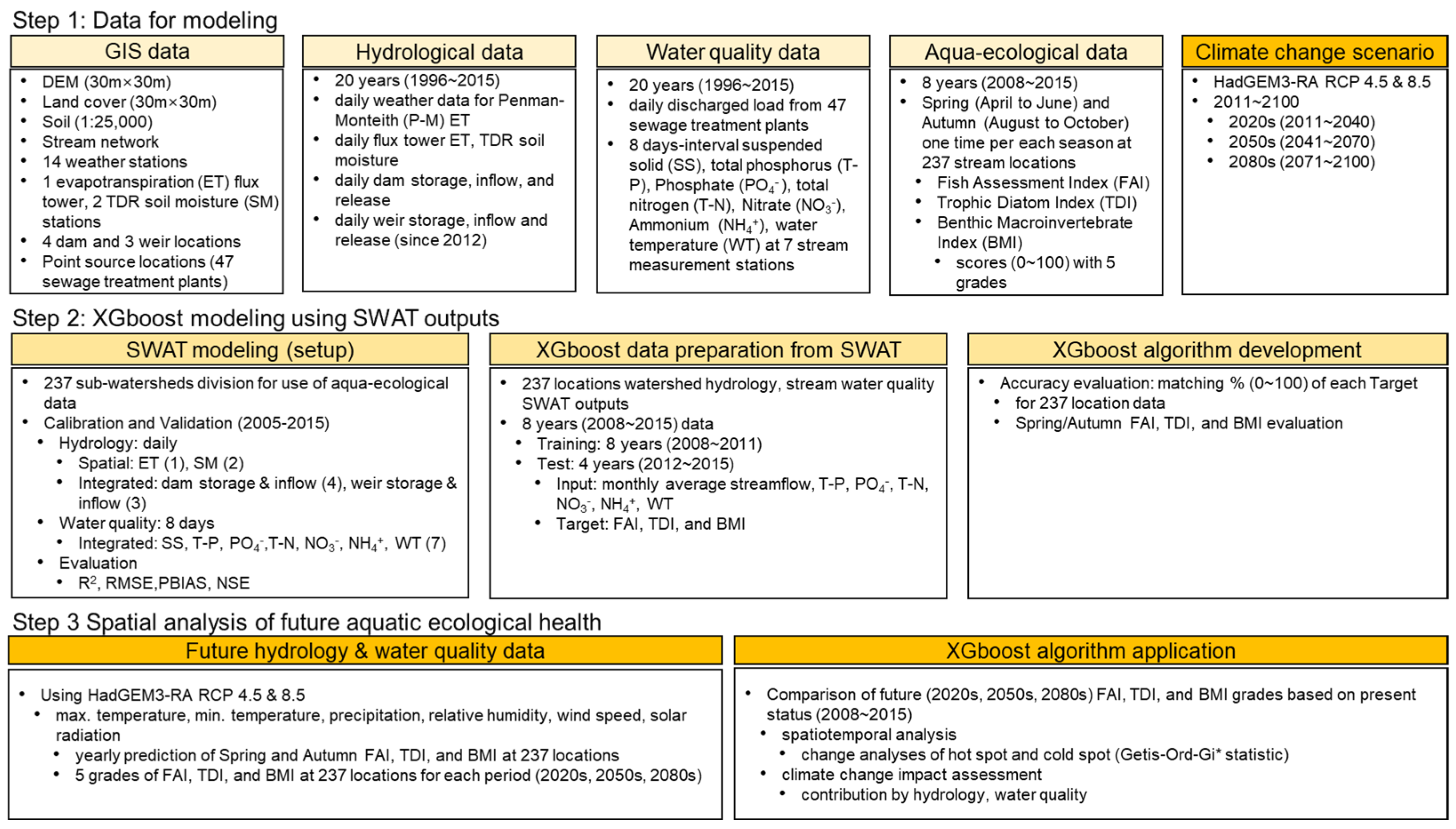
The specific objectives of the study were as follows: (1) calibrate and validate streamflow and water quality of SWAT as input data of XGBoost for estimating ecological health; (2) develop and evaluate the XGboost algorithm for EHI prediction; (3) predict the future EHIs distribution under RCP 4.5 and RCP 8.5 scenarios and analyze the spatio-temporal change in EHIs using hotspot and coldspot (Figure 3). To develop the XGboost algorithm, we used 237 sub-watershed streamflow and water quality results of SWAT as input variables and the grade of EHIs as output variables for 8 years (2008~2015). The total dataset was divided into train data (2008~2011) and test dataset (2012~2015). The future SWAT results were simulated by changing weather conditions based on RCP scenarios, keeping the physical parameters of SWAT.

The SWAT results were used as input variables for the machine learning model because the SWAT model cannot directly simulate decision-making for the estimation of EHIs from hydrological and water quality components. Therefore, this study needs to include the machine learning algorithm. Therefore, the SWAT model provides spatiotemporal flow and water quality with the machine learning algorithm. Additionally, the machine learning algorithm supports decision-making to determine ecological indices with sufficient calibration with respect to flow and water quality.

3. Results and Discussion

3.1. SWAT Calibration and Validation for Estimating Ecological Health

The SWAT model was calibrated and validated based on the hydrology and water quality of seven locations (HSD, SYD, CJD, KCW, YJW, IPW, and PDD) along the main streams using daily inflow data from dams and weirs and monthly water quality data for sediments, T-N, and T-P, respectively. Multi-calibration and validation are helpful for improving the performance of the model by tracing spatial variation in the simulation results [42,43]. The four dams were calibrated for 7 years (2005–2011) and validated for 7 years (2012–2018). The three weirs were calibrated for 3 years (2012–2014) and validated for 4 years (2015–2018), as the weirs have been operated since August 2012.

Before calibrating the model, the sensitive parameters were selected considering the characteristics of the study area based on previous studies [44,45]. To evaluate the availability of the SWAT model, we used the statistical results of the coefficient of determination (R²), Nash–Sutcliffe model efficiency (NSE), and root mean square error (RMSE).

Table 3. Statistical results of SWAT calibration and validation for inflow of structures and water quality.

		(a) HSD	(b) SYD	(c) CJD	(d) KCW	(e) YJW	(f) IPW	(g) PDD
Hydrology
Inflow	NSE	0.68	0.85	0.57	0.37	0.52	0.53	0.71
	R2	0.63	0.79	0.57	0.48	0.50	0.50	0.73
	RMSE	4.28	2.76	3.54	2.03	1.96	1.94	1.98
Water quality (R2)
Sediment		0.54	0.75	0.6	0.42	0.59	0.63	0.63
T-N		0.72	0.81	0.92	0.86	0.83	0.91	0.85
T-P		0.56	0.63	0.75	0.74	0.67	0.75	0.74

shows the SWAT calibration and validation results for daily inflow and monthly water quality at seven stations. The average NSE of inflow was over 0.5, except for KCW, which indicated that the results satisfied the calibration criteria for the NSE [46]. The average R² and RMSE of inflow ranged from 0.48 to 0.79 and from 1.94 to 4.28 mm/day, respectively. Among the calibrated locations, the NSE and R² of the weirs were relatively lower than those for the other structures. This result was because the weirs were calibrated for a relatively short period (7 years), including a severe drought year (2015). The average R² values of sediments, T-N, and T-P were 0.59, 0.84, and 0.69, respectively. The low R² for sediment at KCW was due to the low accuracy of inflow at KCW because runoff influences the sediment yield amount [47].

3.2. Evaluation of Ecological Health by SWAT and XGboost

The EHI distributions in the whole basin were predicted by XGBoost based on the simulated SWAT results of the streamflow, T-N, T-P, NH₄⁺, NO₃⁻, PO₄⁻, and WT of each sub-watershed in spring (April to June) and autumn (August to October). The independent variables for the XGBoost model were SWAT results for 237 subbasins. The output variables were the grades of the Ecological Health Index (EHI), including FAI (Fish Assessment Index), TDI (Trophic Diatom Index), and BMI (Benthic Macroinvertebrate Index), for each of the 237 subbasins. Consequently, the input matrix was structured with nine columns (six SWAT components and three EHI indices) and 237 rows (representing the subbasins). In addition, the data were divided into training (2008 to 2011) and test (2012 to 2015) datasets to minimize overfitting. Then, the XGBoost algorithm conducted parameter tuning using k-fold cross-validation and grid search in Python for eight years (2008 to 2015) to optimize the parameters.

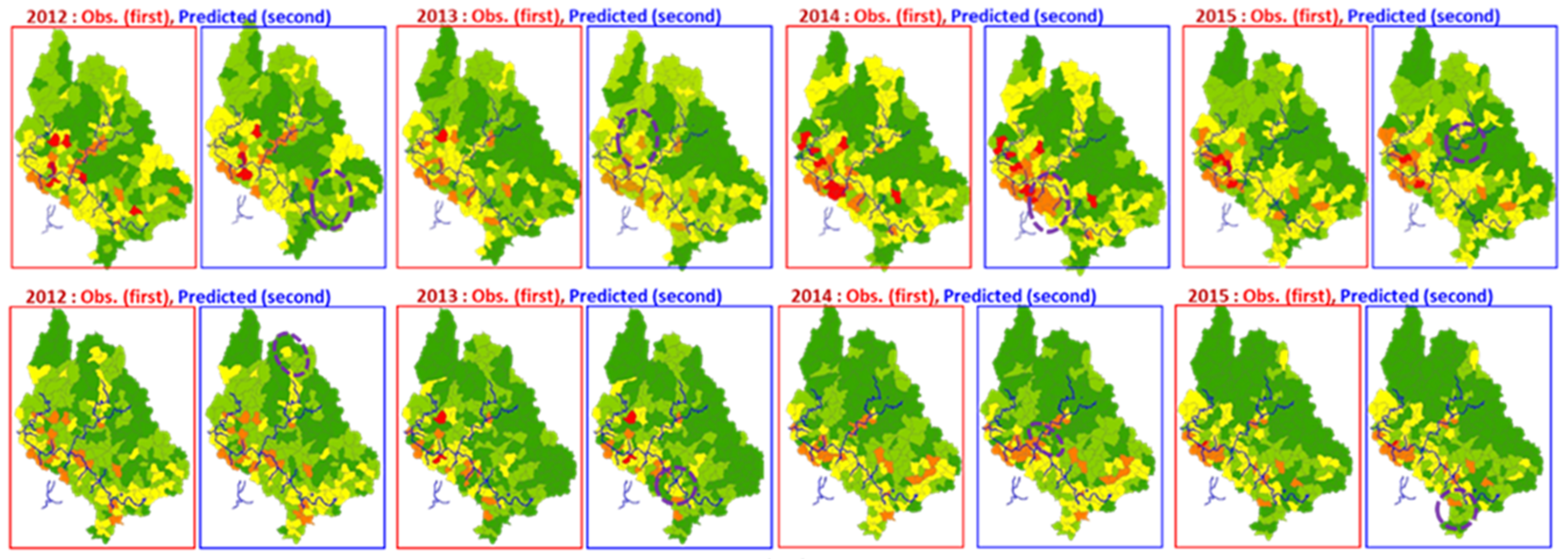
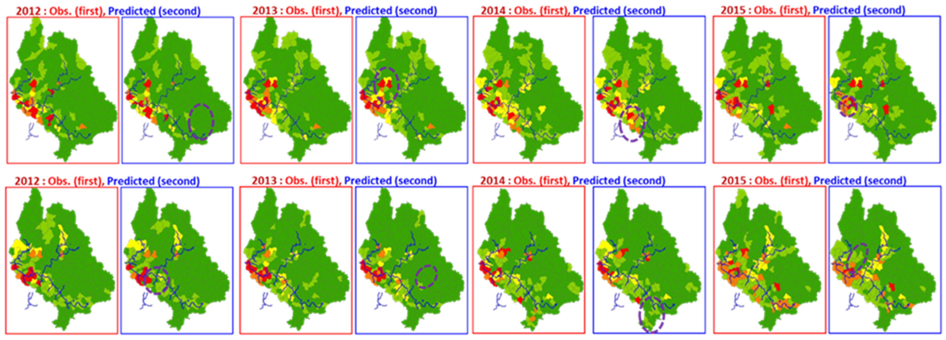
As verified by the test dataset, the average prediction efficiency, expressed as the accuracy value, was 0.72, 0.70, and 0.80 for the FAI, TDI, and BMI, respectively. Afterward, the algorithm predicted the EHIs for the whole simulation period (2008–2015). As seen in Figure 4, Figure 5 and Figure 6, the yearly spatial distribution maps of the EHIs were generated from the average monthly results of SWAT according to seasons (spring and autumn). Dotted circles in Figure 4, Figure 5 and Figure 6 show the sub-watershed, which failed to predict;

Table 4. Summary of the prediction results and average SWAT results (streamflow and water quality components), except for the failed watersheds, for each EHI.

Components	Spring						Autumn
	FAI		TDI		BMI		FAI		TDI		BMI
	True	False	True	False	True	False	True	False	True	False	True	False
Prediction results	89.3%	10.7%	90.8%	9.2%	95.2%	4.8%	93.9%	6.1%	90.4%	9.6%	94.1%	5.9%
Flow (m3/s)	26.7	72.7	27.8	25.2	25.7	26.8	104.3	308.8	110.3	102.1	104.3	104.7
T-N (mg/L)	1.955	1.573	1.952	1.722	1.935	2.754	1.61	1.70	1.607	1.645	1.608	1.704
T-P (mg/L)	0.016	0.021	0.016	0.013	0.015	0.040	0.01	0.02	0.015	0.016	0.015	0.008
NH4+ (mg/L)	0.092	0.118	0.093	0.050	0.091	0.065	0.07	0.10	0.074	0.027	0.072	0.047
NO3− (mg/L)	0.500	0.416	0.499	0.422	0.472	1.743	0.07	0.17	0.072	0.084	0.072	0.126
PO4− (mg/L)	0.010	0.012	0.010	0.006	0.009	0.029	0.009	0.010	0.009	0.011	0.009	0.004
WT (°C)	17.44	17.16	17.44	17.18	17.43	17.40	19.50	19.60	19.47	19.43	19.47	19.49

represents the average prediction failure ratio for 8 years. In each season, the predicted FAI had failure rates of 10.7 and 6.1%. However, the predicted TDI and BMI had similar failure rates in spring and autumn, with values of 9.2% (spring) and 9.6% (autumn) for the TDI and 4.8% (spring) and 5.9% for the BMI (autumn). Table 4 also shows the SWAT-simulated results (streamflow and water quality components) between the successful and failed attempts at predicting the indices in the watersheds. The predicted FAI in spring and autumn showed 171.8% and 196.1% higher flow compared to the flow in the successful watershed. The predicted TDI in spring and autumn showed −45.9% and −63.2% lower NH₄⁺, and the predicted BMI in spring and autumn showed 268.9% and 74.5% higher NO₃ compared to the flow in the successful watershed.

A study predicting daily streamflow in a mountainous watershed using XGBoost concluded that a minimum of 12 years of training data are required for accurate predictions [48]. In this research, the available training data were relatively limited because XGboost was used to predict EHIs, which are observed twice per year. Nevertheless, our results were comparable or superior to those obtained in studies predicting EHI using Random Forest [28] and the WGAN-Based Data Augmentation Method [49]. Additionally, research predicting groundwater levels with XGBoost demonstrated superior performance compared to ANN and SVR methods [50]. In regard to these results, this algorithm linking the SWAT model and the XGBoost algorithm could facilitate decision-making for EHIs. However, the flow, NH₄⁺, and NO₃⁻ were above average, which could cause the poor performance of the algorithm for the prediction of each EHI. Furthermore, due to the inherent black-box nature of XGBoost, this study was unable to clearly identify the various causes of prediction failure. Therefore, this algorithm needs additional variables that are directly relevant to the ecological environment, such as river width, water use facilities, and riverbed conditions, to overcome this lack of information.

3.3. Future Climate Change Impact on Hydrology and Water Quality

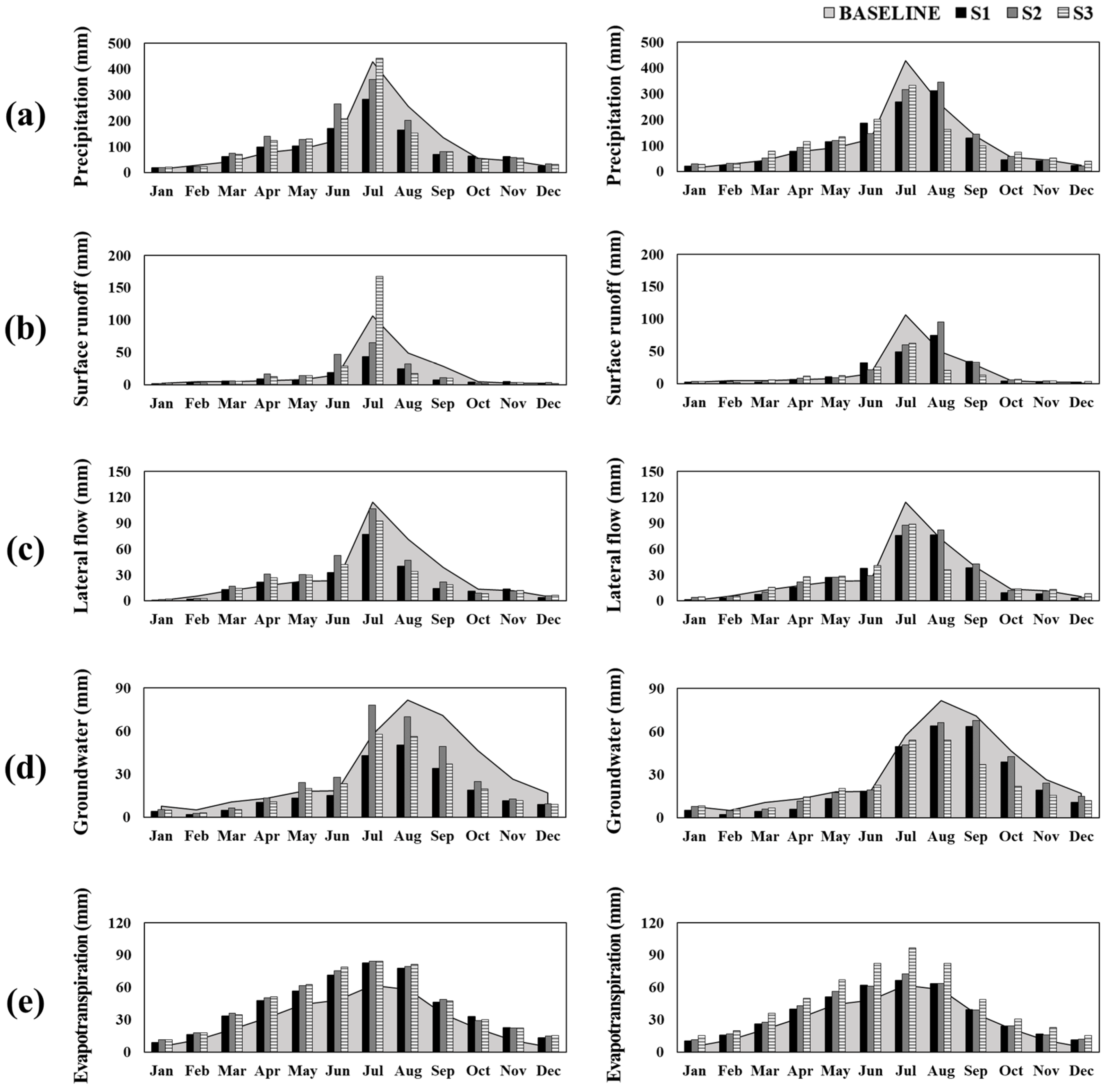
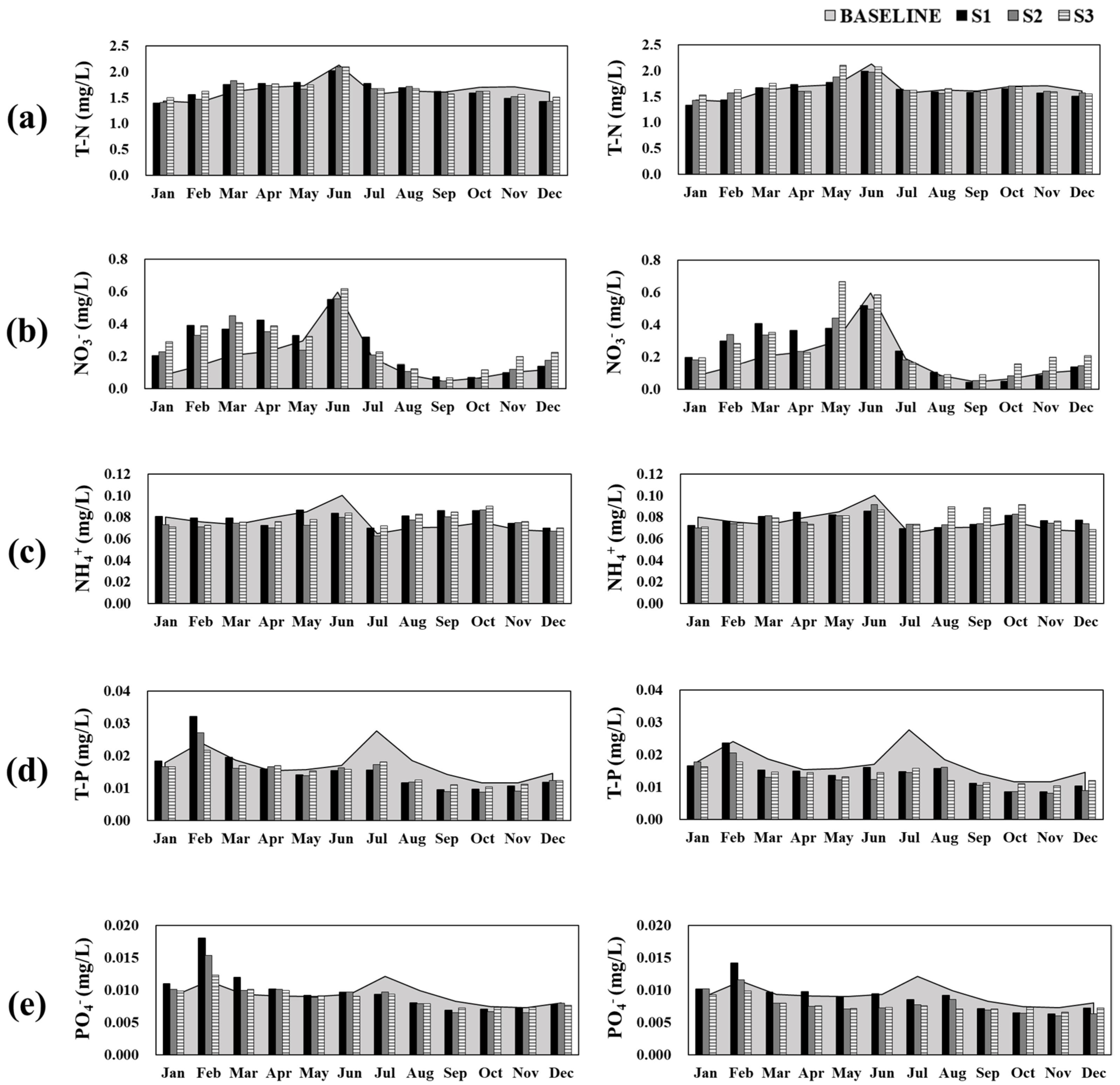
To predict future water cycle and water quality components, the SWAT model was simulated for 90 years (2011–2100) by applying the future climate change RCP4.5 and RCP8.5 scenarios. Figure 7 and Figure 8 represent the monthly average hydrological components and water quality components for the projected periods (Baseline, S1, S2, and S3) under RCP4.5 (left graphs) and RCP8.5 (right graphs).

Surface runoff and lateral flow slightly increased from April to June and decreased from August to October under the RCP4.5 scenario. However, the surface runoff and lateral flow of the RCP8.5 scenario tended to decrease compared to the baseline except in August. Groundwater decreased up to 37 mm per month and 33 mm per month under the RCP4.5 and RCP8.5 scenarios, respectively. However, evapotranspiration increased in all periods in all scenarios, increasing by 3.5 to 31 mm per month in the RCP4.5 scenario and by 2.3 to 34 mm per month in the RCP8.5 scenario.

The target watershed exhibited a marked increase in evapotranspiration due to future climate change, which is attributed to the rise in temperature caused by global warming. Additionally, an increase in spring precipitation was observed, which is expected to alter runoff patterns and consequently impact the future EHIs in spring.

The concentrations of T-N and NH₄⁺ changed slightly under both RCP scenarios. The T-N and NH₄⁺ concentrations changed by −0.22~0.37 mg/L and ±0.02 mg/L, respectively. However, the NO₃⁻ concentration increased by a maximum of 0.25 mg/L before summer because of increased lateral flow and groundwater delivered more NO₃⁻ to streams [51,52]. The concentrations of T-P and PO₄⁻ showed little change except in summer. In the case of the baseline, the concentration increased in summer, but the concentration showed a stable value of approximately 0.015 mg/L under both RCP scenarios.

Climate change encompasses meteorological variations such as changes in precipitation and temperature, which affect the amount of nutrients produced in a watershed. Additionally, these changes influence the discharge of non-point source pollutants due to variations in runoff [53,54]. When applying the RCP scenarios, the increase in spring precipitation led to an increase in runoff, which in turn resulted in higher non-point source pollutant levels and an associated rise in NO₃ concentrations.

3.4. Cold Spot and Hot Spot Analysis of Ecological Health Changes under Future Climate Change

The relationship between ecological health and hydrology has received widespread attention in recent years [55,56]. Climate change exerts multiple pressures on the hydrologic cycle; specifically, it increases the rate of atmospheric water circulation due to increased air temperature and evapotranspiration [57,58,59], and it can cause decreases in groundwater recharge [60,61]. Such changes in the hydrologic cycle in the watershed also affect the water quality [61,62,63] (Eckhard et al., 2003; Luo et al., 2013; Whitehead et al., 2009). Overall, the hydrology and water quality in the upper Han River basin showed a worsening trend under climate change.

Hot spot analysis can create a spatial distribution based on spatial autocorrelation, and this spatial distribution can help to identify spatial patterns and visually compare similarities and differences between regions [64].

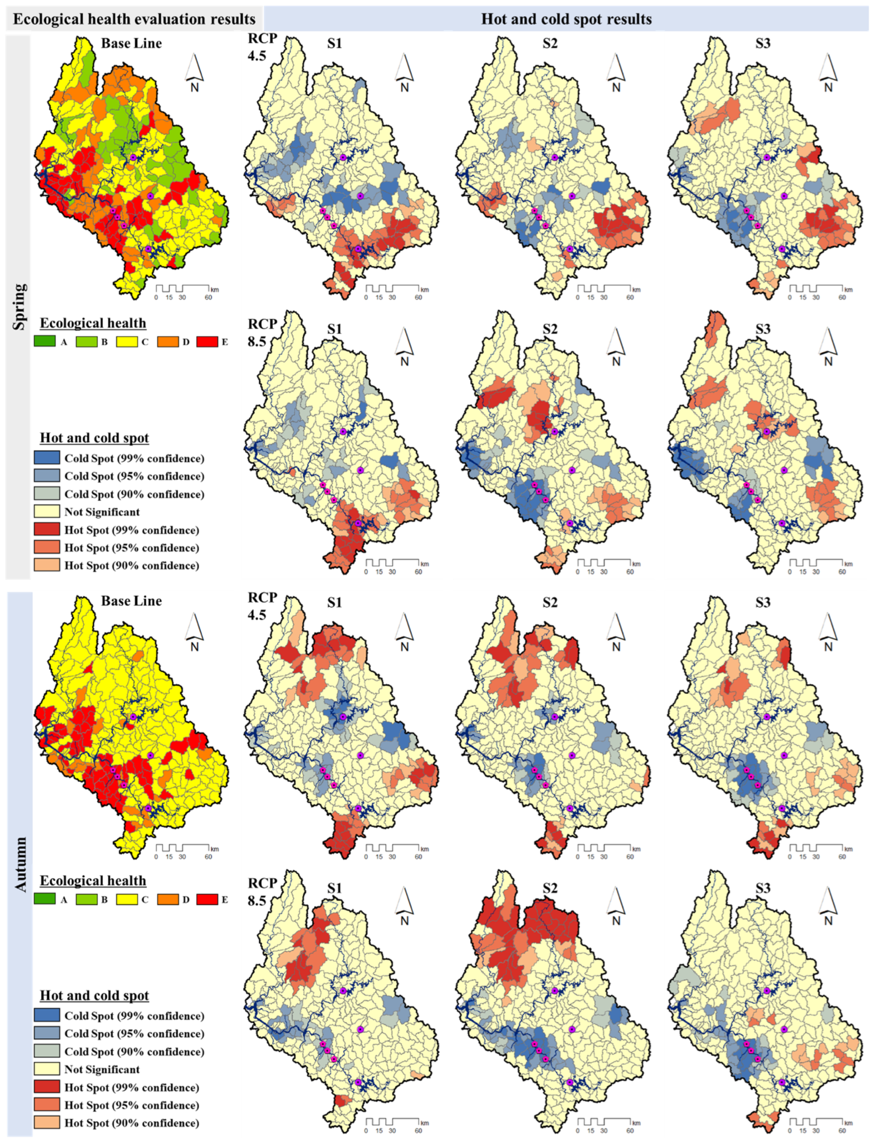
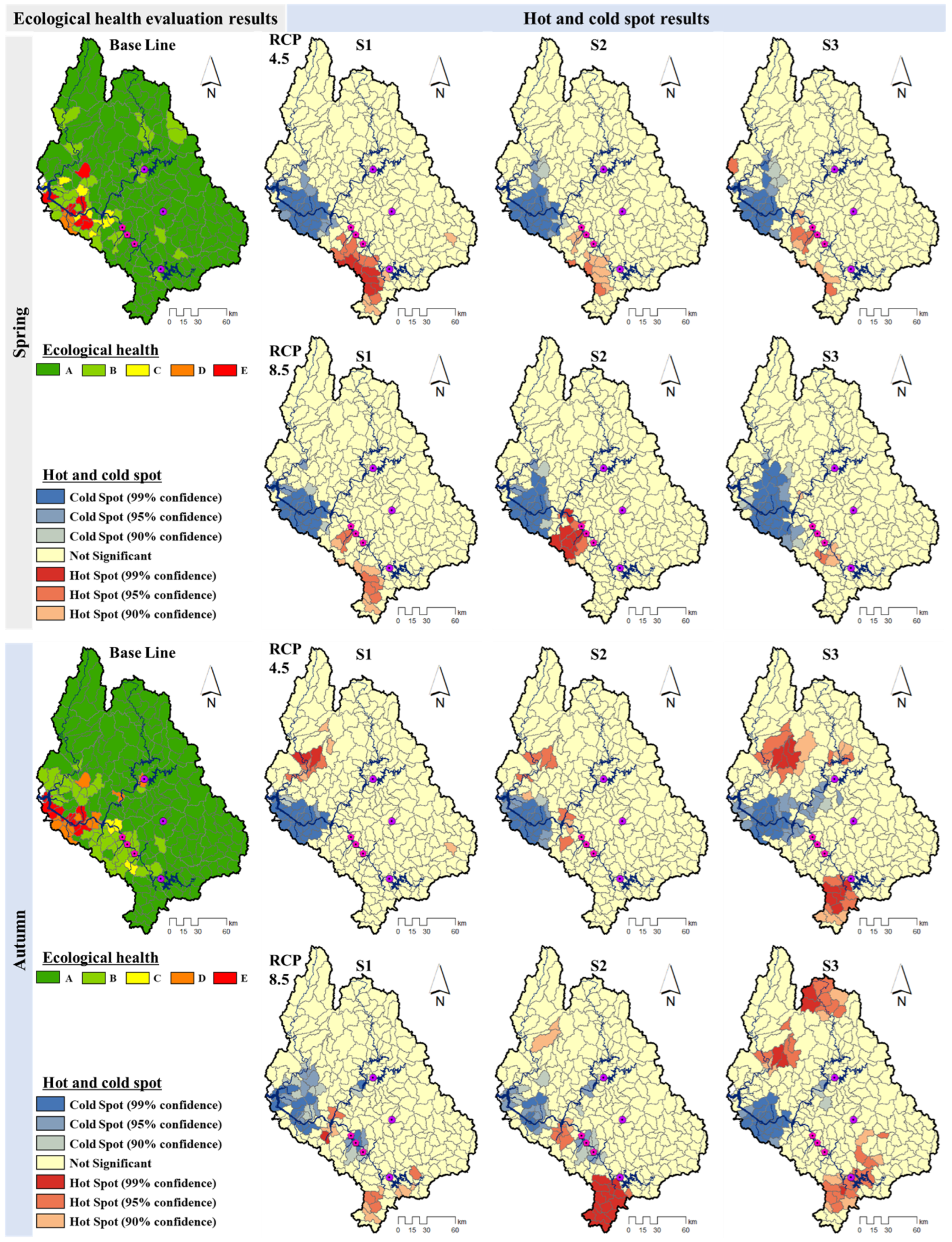
Many studies have used hot spot analysis to assess changes in hydrology and water quality [65,66,67]. The Getis-Ord-Gi* statistic has been widely applied in cold spot and hot spot identification in research areas [67,68,69]. In this study, this method was used to assess the impact of climate change on ecological health. By applying the Getis-Ord-Gi* statistic, hot spot maps of the Han River basin were generated for four projection periods (baseline, S1, S2, and S3). This approach may provide a better understanding of the effect of climate change on ecological health.

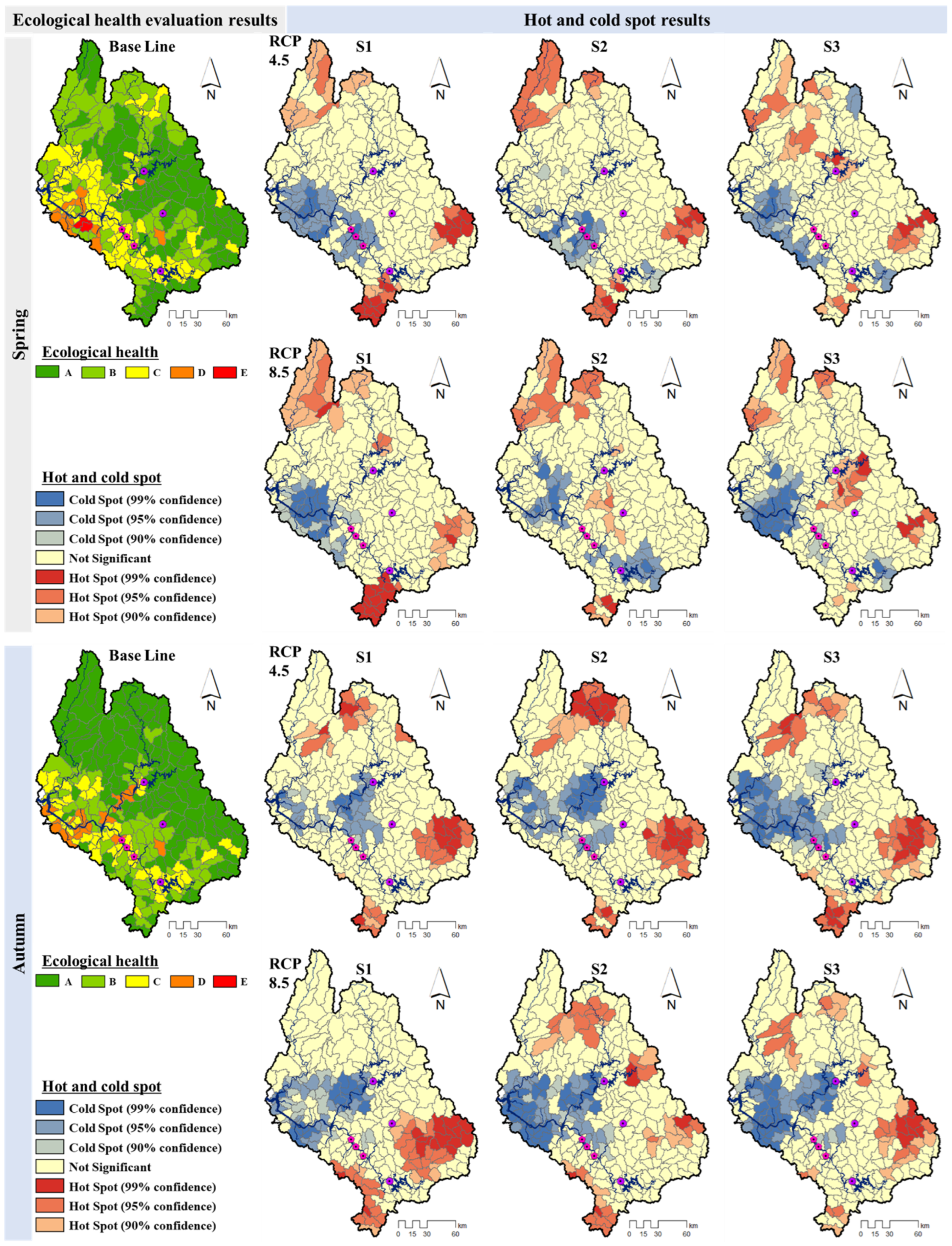
Figure 9, Figure 10 and Figure 11 refer to the analysis of hot spots by index, where hot spots are areas where the ecological index has deteriorated, and cold spots refer to areas where the ecological index has improved. According to a spatial analysis of the change in the FAI compared to the baseline, the FAI health has deteriorated in the upstream branch of the Han River, and the fish ecosystem has improved in the downstream branch of the Han River (Figure 9). The region identified as D or E in the baseline tended to be clustered as a cold spot in the future in the case of the TDI (Figure 10), which was less healthy in the Han River, and the C class tended to be clustered as a hot spot in the future. In the case of the BMI, by spreading the range of cold spots in the future, the health tended to improve in the downstream region of the Han River (Figure 11). In the upstream reach of the Han River, the future BMI was degraded and appeared to be clustered as a hot spot, and the class A region of the baseline shifted to class B and became a hot spot. Most of the cold spot results by EHIs were represented in the downstream areas, or the areas with hydraulic structures (dams and weirs) were identified as class D or E in the baseline period. It implied that areas that used to be detrimental to health in the past could not get worse because the developed SWAT-XGboost linkage algorithm was trained from class A to E. And it showed that the areas with class C tended to deteriorate gradually. Therefore, it is necessary to manage the integrated water environment, including hydrology, water quality, and aquatic ecological health in order to prevent future ecological health conditions from deteriorating.

4. Conclusions

This study aimed to develop a SWAT-XGBoost linkage algorithm to estimate spatiotemporal EHIs using observed monitoring data and SWAT-simulated data and analyze the changes in future EHIs under RCP scenarios (RCP4.5 and 8.5) in the river system of the Han River watershed (34,148 km²) using the newly developed SWAT-XGBoost linkage algorithm. The main results derived from this study are as follows:

1. The SWAT model was calibrated for streamflow and water quality (sediment, T-N, and T-P) components at seven points in the Han River basin. As a result, the NSE, R², and RMSE of the streamflow were 0.61, 0.6, and 2.6 mm/day, respectively. The R² values for sediment, T-N, and T-P were 0.59, 0.84, and 0.69, respectively.

2. The developed SWAT-XGBoost linkage was verified by comparing the observed EHIs at the watershed scale. With 89.3 to 95.2% accuracy, the method used in this study overcame the limitations of using only the model and simple regression by improving both the bias and the variance of the EHI estimation as a new approach. Nevertheless, there were not enough data on most of the subwatersheds. In addition, this study could not clearly identify various causes in terms of prediction failure since XGBoost has the general features of a black box model. Therefore, this study should acquire the data that are related to the ecological environment, help train the XGBoost algorithm, and then reanalyze the results in an area that showed a prediction failure.

3. The future water cycle components showed steady increases in evapotranspiration (2.3~34 mm) due to increased temperature and notable changes in streamflow before and after the summer monsoon compared to the baseline. The significant change in the future water quality concentration was an increase in NO₃⁻ from January to June, which increased up to 0.25 mg/L.

4. The cold and hot spot analysis for the future EHIs showed that ecological health deteriorated in the upstream area of the Han River basin due to changes in hydrology and water quality (T-N, T-P, NH₄⁺, NO₃⁻, PO₄⁻). However, the downstream regions ranked as D or E in the baseline case tended to be clustered as cold spots because the developed algorithm cannot predict the phenomena that will be more deteriorated than the E class.

This study evaluates the direction of future aquatic changes in watershed units through a combination of machine learning and hydrological models. This approach is economical because the calculation time is faster than the original complex EHI approach for estimation, and various interpretations of hydrology, water quality, and aquatic ecology can be performed. However, if the SWAT model could consider other ecological components, such as river width, water use facilities, and riverbed conditions, this method would be a more useful approach for the study of EHI changes. In addition, this approach will help both water resource managers and local stakeholders prioritize and establish strategies for the protection and restoration of a watershed by evaluating future changes. Future research should focus on restoration and adaptation measures against climate change to sustain stable flow and water quality in vulnerable areas.

References

- Trenberth, K.E. Conceptual framework for changes of extremes of the hydrological cycle with climate change. Clim. Change 1999, 42, 327–339. [Google Scholar] [CrossRef]
- Trenberth, K.E. Changes in precipitation with climate change. Clim. Res. 2011, 47, 123–138. [Google Scholar]
- O’neil, J.; Davis, T.W.; Burford, M.A.; Gobler, C. The rise of harmful cyanobacteria blooms: The potential roles of eutrophication and climate change. Harmful Algae 2012, 14, 313–334. [Google Scholar]
- Peperzak, L. Climate change and harmful algal blooms in the North Sea. Acta Oecol. 2003, 24, S139–S144. [Google Scholar]
- Hung, C.L.J.; James, L.A.; Carbone, G.J.; Williams, J.M. Impacts of combined land-use and climate change on streamflow in two nested catchments in the Southeastern United States. Ecol. Eng. 2020, 143, 105665. [Google Scholar]
- Kiesel, J.; Gericke, A.; Rathjens, H.; Wetzig, A.; Kakouei, K.; Jähnig, S.C.; Fohrer, N. Climate change impacts on ecologically relevant hydrological indicators in three catchments in three European ecoregions. Ecol. Eng. 2019, 127, 404–416. [Google Scholar]
- Peraza-Castro, M.; Ruiz-Romera, E.; Meaurio, M.; Sauvage, S.; Sánchez-Pérez, J.M. Modelling the impact of climate and land cover change on hydrology and water quality in a forest watershed in the Basque Country (Northern Spain). Ecol. Eng. 2018, 122, 315–326. [Google Scholar]
- Hötzel, G.; Croome, R. A Phytoplankton Methods Manual for Australian Freshwaters; LWRRDC Occasional Paper. 22/99; Land and Water Resources Research and Development Corporation: Canberra, Australia, 1999. [Google Scholar]
- Domingues, R.; Galvao, H. Phytoplankton and environmental variability in a dam regulated temperate estuary. Hydrobiologia 2007, 586, 117–134. [Google Scholar]
- Cabecinha, E.; Cortes, R.; Cabral, J.; Ferreira, T.; Lourenço, M.; Pardal, M. Multiscale approach using phytoplankton as a first step towards the definition of the ecological status of reservoirs. Ecol. Indic. 2009, 9, 240–255. [Google Scholar]
- Aazami, J.; Esmaili-Sari, A.; Abdoli, A.; Sohrabi, H.; Van den Brink, P.J. Monitoring and assessment of water health quality in the Tajan River, Iran using physicochemical, fish and macroinvertebrates indices. J. Environ. Health Sci. Eng. 2015, 13, 29. [Google Scholar]
- Cheimonopoulou, M.T.; Bobori, D.C.; Theocharopoulos, I.; Lazaridou, M. Assessing ecological water quality with macroinvertebrates and fish: A case study from a small Mediterranean river. Environ. Manag. 2011, 47, 279–290. [Google Scholar] [CrossRef] [PubMed]
- Kelly, M.G.; Whitton, B.A. The trophic diatom index: A new index for monitoring eutrophication in rivers. J. Appl. Phycol. 1995, 7, 433–444. [Google Scholar]
- Schultz, R.; Dibble, E. Effects of invasive macrophytes on freshwater fish and macroinvertebrate communities: The role of invasive plant traits. Hydrobiologia 2012, 684, 1–14. [Google Scholar] [CrossRef]
- United States Environmental Protection Agency (U.S. EPA). Fish Field and Laboratory Methods for Evaluating the Biological Integrity of Surface Waters; EPA 600-R-92-111; U.S. EPA: Washington, DC, USA, 1993.
- Merritt, R.W.; Cummins, K.W. An Introduction to the Aquatic Insects of North America, 2nd ed.; Kendall Hunt Publishing Co.: Dubuque, IA, USA, 1984; Volume 862. [Google Scholar]
- Karandish, F.; Simunek, J. A comparison of numerical and machine-learning modeling of soil water content with limited input data. J. Hydrol. 2016, 543, 892–909. [Google Scholar] [CrossRef]
- Riad, S.; Mania, J.; Bouchaou, L.; Najjar, Y. Rainfall-runoff model using an artificial neural network approach. Math. Comput. Modell. 2004, 40, 839–846. [Google Scholar]
- Mehr, A.D.; Nourani, V. A Pareto-optimal moving average-multigene genetic programming model for rainfall-runoff modelling. Environ. Modell. Softw. 2017, 92, 239–251. [Google Scholar]
- Ni, L.; Wang, D.; Wu, J.; Wang, Y.; Tao, Y.; Zhang, J.; Liu, J. Streamflow forecasting using extreme gradient boosting model coupled with Gaussian mixture model. J. Hydrol. 2020, 586, 124901. [Google Scholar] [CrossRef]
- French, J.; Mawdsley, R.; Fujiyama, T.; Achuthan, K. Combining machine learning with computational hydrodynamics for prediction of tidal surge inundation at estuarine ports. Procedia IUTAM 2017, 25, 28–35. [Google Scholar]
- Khan, N.; Sachindra, D.A.; Shahid, S.; Ahmed, K.; Shiru, M.S.; Nawaz, N. Prediction of droughts over Pakistan using machine learning algorithms. Adv. Water Resour. 2020, 139, 103562. [Google Scholar]
- Bhattacharya, B.; Price, R.K.; Solomatine, D.P. Machine learning approach to modeling sediment transport. J. Hydraul. Eng. 2007, 133, 440–450. [Google Scholar]
- Ebtehaj, I.; Bonakdari, H.; Zaji, A.H.; Bong, C.H.J.; Ab Ghani, A. Design of a new hybrid artificial neural network method based on decision trees for calculating the Froude number in rigid rectangular channels. J. Hydrol. Hydromech. 2016, 64, 252–260. [Google Scholar] [CrossRef]
- Kim, R.J.; Loucks, D.P.; Stedinger, J.R. Artificial neural network models of watershed nutrient loading. Water Resour. Manag. 2012, 26, 2781–2797. [Google Scholar] [CrossRef]
- Park, Y.S.; Verdonschot, P.F.; Chon, T.S.; Lek, S. Patterning and predicting aquatic macroinvertebrate diversities using artificial neural network. Water Res. 2003, 37, 1749–1758. [Google Scholar] [CrossRef]
- Gebler, D.; Wiegleb, G.; Szoszkiewicz, K. Integrating river hydromorphology and water quality into ecological status modelling by artificial neural networks. Water Res. 2018, 139, 395–405. [Google Scholar] [CrossRef] [PubMed]
- Woo, S.Y.; Jung, C.G.; Lee, J.W.; Kim, S.J. Evaluation of Watershed Scale Aquatic Ecosystem Health by SWAT Modeling and Random Forest Technique. Sustainability 2019, 11, 3397. [Google Scholar] [CrossRef]
- Cisty, M.; Soldanova, V. Flow prediction versus flow simulation using machine learning algorithms. In Machine Learning and Data Mining in Pattern Recognition, Proceedings of the 14th International Conference, MLDM 2018, New York, NY, USA, 15–19 July 2018; Proceedings, Part II 14; Springer International Publishing: Berlin/Heidelberg, Germany, 2018; pp. 369–382. [Google Scholar]
- White, E. Predicting Unimparied Flow in Ungauged Basins: “Random Forests” Applied to California Streams. Master’s Thesis, University of Kentucky, Lexington, KY, USA, 2015. [Google Scholar]
- Lee, S.W.; Hwang, S.J.; Lee, J.K.; Jung, D.I.; Park, Y.J.; Kim, J.T. Overview and application of the national aquatic ecological monitoring program (NAEMP) in Korea. Ann. Limnol. Int. J. Lomnol. 2011, 47, S3–S14. [Google Scholar]
- Ministry of Environment. Nationwide Aquatic Ecological Monitoring Program; National Institute of Environmental Research: Incheon, Republic of Korea, 2015.
- IPCC. Climate Change 2013: The Physical Science Basis Contribution of Working Group I to the Fifth Assessment Report of the Intergovernmental Panel on Climate Change; Stocker, T.F., Qin, D., Plattner, G.-K., Tignor, M., Allen, S.K., Boschung, J., Nauels, A., Xia, Y., Bex, V., Midgley, P.M., Eds.; Cambridge University Press: Cambridge, UK; New York, NY, USA, 2013; 1535p. [Google Scholar] [CrossRef]
- Arnold, J.G.; Srinivasan, R.; Muttiah, R.S.; Williams, J.R. Large area hydrologic modelling and assessment part I: Model development. J. Am. Water Resour. Assoc. 1998, 34, 73–89. [Google Scholar] [CrossRef]
- Neitsch, S.L.; Arnold, J.G.; Kiniry, J.R.; Williams, J.R.; King, K.W. Soil and Water Assessment Tool Theoretical Documentation: Version 2009; Texas Water Resources Institute: College Station, TX, USA, 2011. [Google Scholar]
- USDA Soil Conservation Service. National Engineering Handbook. Hydrology Section 4; Chapters 4–10; U.S. Government Printing Office: Washington, DC, USA, 1972.
- Williams, J.R. Sediment-Yield Prediction with Universal Equation Using Runoff Energy Factor, Present and Prospective Technology for Predicting Sediment Yield and Sources; Proceedings of the Sediment-Yield Workshop; USDA Sedimentation Lab: Oxford, MS, USA, 1975.
- Brown, L.C.; Barnwell, T.O. The Enhanced Stream Water Quality Models QUAL2E and QUAL2E-UNCAS: Documentation and User Manual; EPA: Washington, DC, USA, 1987; Volume 600, pp. 3–87.
- Chen, T.; Guestrin, C. Xgboost: A scalable tree boosting system. In Proceedings of the 22nd ACM Sigkdd International Conference on Knowledge Discovery and Data Mining, San Francisco, CA, USA, 13–17 August 2016; pp. 785–794. [Google Scholar]
- Mitchell, M.G.; Suarez-Castro, A.F.; Martinez-Harms, M.; Maron, M.; McAlpine, C.; Gaston, K.J.; Johansen, K.; Rhodes, J.R. Reframing landscape fragmentation’s effects on ecosystem services. Trends Ecol. Evol. 2015, 30, 190–198. [Google Scholar]
- Jana, M.; Sar, N. Modeling of hotspot detection using cluster outlier analysis and Getis-Ord Gi* statistic of educational development in upper-primary level, India. Model. Earth Syst. Environ. 2016, 2, 60. [Google Scholar]
- Santhi, C.; Arnold, J.G.; Williams, J.R.; Hauck, L.M.; Dugas, W.A. Application of a watershed model to evaluate management effects on point and nonpoint source pollution. Trans. ASAE 2001, 44, 1559. [Google Scholar]
- White, K.L.; Chaubey, I. Sensitivity analysis, calibration, and validations for a multisite and multivariable SWAT model. J. Am. Water Resour. Assoc. 2005, 41, 1077–1089. [Google Scholar]
- Ahn, S.R.; Lee, J.W.; Jang, S.S.; Kim, S.J. Large Scale SWAT Watershed Modeling Considering Multi-Purpose Dams and Multi-Function Weirs Operation-For Namhan River Basin. J. Korean Soc. Agric. Eng. 2016, 58, 21–35. (In Korean) [Google Scholar]
- Ahn, S.R. Physically Based Watershed Health Resilience Assessment Considering Climate Change. Ph.D. Thesis, Graduate School of Konkuk University, Seoul, Republic of Korea, 2016. [Google Scholar]
- Moriasi, D.N.; Arnold, J.G.; Van Liew, M.W.; Bingner, R.L.; Harmel, R.D.; Veith, T.L. Model evaluation guidelines for systematic quantification of accuracy in watershed simulations. Trans. ASABE 2007, 50, 885–900. [Google Scholar]
- Zeiger, S.J.; Hubbart, J.A. A SWAT model validation of nested-scale contemporaneous stream flow, suspended sediment and nutrients from a multiple-land-use watershed of the central USA. Sci. Total Environ. 2016, 572, 232–243. [Google Scholar] [PubMed]
- Szczepanek, R. Daily streamflow forecasting in mountainous catchment using XGBoost, LightGBM and CatBoost. Hydrology 2022, 9, 226. [Google Scholar] [CrossRef]
- Lee, S.; Kim, J.; Lee, G.; Hong, J.; Bae, J.H.; Lim, K.J. Prediction of aquatic ecosystem health indices through machine learning models using the WGAN-based data augmentation method. Sustainability 2021, 13, 10435. [Google Scholar] [CrossRef]
- Osman, A.I.A.; Ahmed, A.N.; Chow, M.F.; Huang, Y.F.; El-Shafie, A. Extreme gradient boosting (Xgboost) model to predict the groundwater levels in Selangor Malaysia. Ain Shams Eng. J. 2021, 12, 1545–1556. [Google Scholar]
- Hallberg, G.R. Nitrates in ground water in Iowa. In Rural Ground Water Contamination; D’Itri, F.M., Wolfson, L.G., Eds.; Lewis: Chelsea, MI, USA, 1987; pp. 23–68. [Google Scholar]
- Schilling, K.E. Chemical transport from paired agricultural and restored prairie watersheds. J. Environ. Qual. 2002, 31, 1184–1193. [Google Scholar] [CrossRef] [PubMed]
- Badrzadeh, N.; Samani, J.M.V.; Mazaheri, M.; Kuriqi, A. Evaluation of management practices on agricultural nonpoint source pollution discharges into the rivers under climate change effects. Sci. Total Environ. 2022, 838, 156643. [Google Scholar] [CrossRef]
- Wang, Y.; Bian, J.; Zhao, Y.; Tang, J.; Jia, Z. Assessment of future climate change impacts on nonpoint source pollution in snowmelt period for a cold area using SWAT. Sci. Rep. 2018, 8, 2402. [Google Scholar] [CrossRef]
- John, A.; Horne, A.; Nathan, R.; Stewardson, M.; Webb, J.A.; Wang, J.; Poff, N.L. Climate change and freshwater ecology: Hydrological and ecological methods of comparable complexity are needed to predict risk. Wiley Interdiscip. Rev. Clim. Change 2021, 12, e692. [Google Scholar]
- Vollmer, D.; Shaad, K.; Souter, N.J.; Farrell, T.; Dudgeon, D.; Sullivan, C.A.; Regan, H.M. Integrating the social, hydrological and ecological dimensions of freshwater health: The Freshwater Health Index. Sci. Total Environ. 2018, 627, 304–313. [Google Scholar] [PubMed]
- Chu, J.T.; Xia, J.; Xu, C.Y.; Singh, V.P. Statistical downscaling of daily mean temperature, pan evaporation and precipitation for climate change scenarios in Haihe River China. Theor. Appl. Climatol. 2010, 99, 149–161. [Google Scholar] [CrossRef]
- O’Gorman, P.A.; Schneider, T. The physical basis for increases in precipitation extremes in simulations of 21st-century climate change. Proc. Natl. Acad. Sci. USA 2009, 106, 14773–14777. [Google Scholar] [CrossRef] [PubMed]
- Tabari, H. Climate change impact on flood and extreme precipitation increases with water availability. Sci. Rep. 2020, 10, 13768. [Google Scholar]
- Condon, L.E.; Atchley, A.L.; Maxwell, R.M. Evapotranspiration depletes groundwater under warming over the contiguous United States. Nat. Commun. 2020, 11, 873. [Google Scholar] [PubMed]
- Eckhardt, K.; Ulbrich, U.J.J.O.H. Potential impacts of climate change on groundwater recharge and streamflow in a central European low mountain range. J. Hydrol. 2003, 284, 244–252. [Google Scholar]
- Luo, Y.; Ficklin, D.L.; Liu, X.; Zhang, M. Assessment of climate change impacts on hydrology and water quality with a watershed modeling approach. Sci. Total Environ. 2013, 450, 72–82. [Google Scholar]
- Whitehead, P.G.; Wilby, R.L.; Battarbee, R.W.; Kernan, M.; Wade, A.J. A review of the potential impacts of climate change on surface water quality. Hydrol. Sci. J. 2009, 54, 101–123. [Google Scholar] [CrossRef]
- Getis, A.; Ord, J.K. The analysis of spatial association by use of distance statistics. Geogr. Anal. 1992, 24, 189–206. [Google Scholar] [CrossRef]
- Desbureaux, S.; Mortier, F.; Zaveri, E.; van Vliet, M.T.; Russ, J.; Rodella, A.S.; Damania, R. Mapping global hotspots and trends of water quality (1992–2010): A data driven approach. Environ. Res. Lett. 2022, 17, 114048. [Google Scholar]
- Peng, L.C.; Lin, Y.P.; Chen, G.W.; Lien, W.Y. Climate change impact on spatiotemporal hotspots of hydrologic ecosystem services: A case study of Chinan catchment, Taiwan. Water 2019, 11, 867. [Google Scholar] [CrossRef]
- Zabaleta, B.; Achkar, M.; Aubriot, L. Hotspot analysis of spatial distribution of algae blooms in small and medium water bodies. Environ. Monit. Assess. 2021, 193, 1–25. [Google Scholar]
- Badlowski, G.A.; Adolf, J.E.; Fouad, G. Spatial analysis of water quality parameters in Hilo Bay, Hawai’i, using a combination of interpolated surfaces and hot spot analysis. Environ. Monit. Assess. 2021, 193, 118. [Google Scholar] [CrossRef]
- Xu, B.; Qi, B.; Ji, K.; Liu, Z.; Deng, L.; Jiang, L. Emerging hot spot analysis and the spatial–temporal trends of NDVI in the Jing River Basin of China. Environ. Earth Sci. 2022, 81, 55. [Google Scholar]
Figure 1.
Location of the study area (Han River watershed) and distribution of weather station, aquatic ecology, point source pollution, and water quality monitoring sites.
Figure 2.
Monthly average precipitation and maximum and minimum air temperatures for four periods (historical: 1976–2005; 2020s: 2011–2040; 2050s: 2041–2070; 2080s: 2071–2100) under the (a) RCP4.5 and (b) RCP8.5 scenarios.
Figure 3.
Flow chart of the study.
Figure 4.
The comparison between observed and predicted FAI in spring (top) and autumn (bottom) during 2012–2015.
Figure 5.
The comparison between observed and predicted TDI in spring (top) and autumn (bottom) during 2012–2015.
Figure 6.
The comparison between observed and predicted BMI in spring (top) and autumn (bottom) during 2012–2015.
Figure 7.
Comparison of monthly average water cycle components: (a) precipitation, (b) surface runoff, (c) lateral flow, (d) groundwater, and (e) evapotranspiration, calculated from the SWAT results under the RCP4.5 (left graphs) and RCP8.5 (right graphs) scenarios.
Figure 8.
Comparison of monthly average water quality concentrations of (a) T-N, (b) NO3−, (c) NH4+, (d) T-P, and (e) PO4− calculated from the SWAT results under the RCP4.5 (left graphs) and RCP8.5 (right graphs) scenarios.
Figure 9.
Hot and cold spot analysis results of the FAI.
Figure 10.
Hot and cold spot analysis results of the TDI.
Figure 11.
Hot and cold spot analysis results of the BMI.