Article

A Water Demand Forecasting Model Based on Generative Adversarial Networks and Multivariate Feature Fusion

1
School of Microelectronics and Control Engineering, Changzhou University, Changzhou 213164, China
2
College of Information Science and Technology, Zhejiang Shuren University, Hangzhou 310015, China
*
Author to whom correspondence should be addressed.
Water 2024, 16(12), 1731; https://doi.org/10.3390/w16121731
Submission received: 28 May 2024 / Revised: 14 June 2024 / Accepted: 15 June 2024 / Published: 19 June 2024
(This article belongs to the Section Urban Water Management)

Abstract

:
Accurate long-term water demand forecasting is beneficial to the sustainable development and management of cities. However, the randomness and nonlinear nature of water demand bring great challenges to accurate long-term water demand forecasting. For accurate long-term water demand forecasting, the models currently in use demand the input of extensive datasets, leading to increased costs for data gathering and higher barriers to entry for predictive projects. This situation underscores the pressing need for an effective forecasting method that can operate with a smaller dataset, making long-term water demand predictions more feasible and economically sensible. This study proposes a framework to delineate and analyze long-term water demand patterns. A forecasting model based on generative adversarial networks and multivariate feature fusion (the water demand forecast-mixer, WDF-mixer) is designed to generate synthetic data, and a gradient constraint is introduced to overcome the problem of overfitting. A multi-feature fusion method based on temporal and channel features is then derived, where a multi-layer perceptron is used to capture temporal dependencies and non-negative matrix decomposition is applied to obtain channel dependencies. After that, an attention layer receives all those features associated with the water demand forecasting, guiding the model to focus on important features and representing correlations across them. Finally, a fully connected network is constructed to improve the modeling efficiency and output the forecasting results. This approach was applied to real-world datasets. Our experimental results on four water demand datasets show that the proposed WDF-mixer model can achieve high forecasting accuracy and robustness. In comparison to the suboptimal models, the method introduced in this study demonstrated a notable enhancement, with a 62.61% reduction in the MSE, a 46.85% decrease in the MAE, and a 69.15% improve in the R 2 score. This research could support decision makers in reducing uncertainty and increasing the quality of water resource planning and management.

1. Introduction

With the development of the social economy, the contradiction between supply of and demand for urban water resources is increasing. The forecasting of water demand is of profound significance in urban water management planning and urban comprehensive development planning [1,2]. The study of water demand forecasting is an important component of and a fundamental prerequisite to ensuring the optimal operation of water supply networks [3,4]. By accurately forecasting changes in water demand at the water supply network’s nodes, we can better plan and manage the operation of urban water supply and drainage pipe networks, improve the safety and reliability of the pipe network, reduce leakage and waste, and ensure the stability of water supply.
The most common methods for water demand forecasting include regression analysis, traditional time series analysis, and artificial neural networks. Regression analysis methods forecast future water demand by establishing a regression model between water demand and relevant influencing factors [5,6]. However, due to the highly nonlinear nature of water demand sequences, it is difficult to accurately model water demand based on linear regression models. The traditional time series analysis method selects an appropriate model to fit the change pattern of historical data in order to describe the changing trend of the data [7,8,9,10]. Although this method is easy to implement, its models are not easily interpretable and are highly dependent on historical data. If the sample size of the historical data is small or the data quality is poor, the forecasting accuracy will experience a cliff-like decline. Artificial neural networks learn the characteristics and patterns of changes in historical water demand through connections and weights between neurons, and they then forecast future water demand based on the learned models [11,12,13,14]. Compared to other methods, artificial neural networks have stronger nonlinear modeling abilities and adaptability, enabling them to process more complex time series data. However, when the dataset has data quality issues or is a small size, artificial neural networks are prone to overfitting, leading to a decrease in forecasting accuracy. The forecasting of urban water demand is influenced by many factors, including environmental factors, historical water demand, and the water demand of the surrounding nodes. Traditional methods for water demand forecasting rely solely on historical water usage data. The quantity and quality of this data can greatly affect the forecasting accuracy. Forecasting accuracy often decreases rapidly as the time range increases, making long-term water demand forecasting difficult to achieve.
The limitations of traditional forecasting methods have led scholars to conduct research on multivariate water demand forecasting methods. Guo [15] proposed a new hybrid model for urban water demand forecasting, which employed the random forest method for data dimensionality reduction to eliminate unimportant influencing factors, utilized discrete wavelet transform to decompose the original sequence into several sub-sequences with different characteristics, and applied a time convolutional network to model multiple sub-sequences to generate forecasting results. The model demonstrated excellent predictive performance on a real dataset provided by a water plant in Suzhou, China, proving the reliability of using multivariate sequences for forecasting. Compared to the methods mentioned above, Transformer-based models that capture long-term dependencies have gradually become the mainstream model in the field of water demand forecasting. Many Transformer variant architectures have been designed for long-term time series forecasting modeling tasks. Zhou [16] proposed the Informer model, which first applies the Transformer architecture to the field of long-term time series forecasting and introduces a sparse self-attention mechanism to reduce the model’s time complexity. Extensive experiments on multiple large-scale datasets confirmed the reliability of the Transformer architecture in the field of long-term time series forecasting. Wu [17] addressed the issue of low information utilization of the sparse self-attention mechanism by proposing a new decomposition architecture with an auto-correlation mechanism in the Autoformer model, progressively decomposing complex time series. The Autoformer model achieved better forecasting results than the Informer on multiple datasets in the five categories of time series forecasting tasks. Zhou [18] combined the Transformer with a seasonal trend decomposition method, further improving the long-term forecasting performance of the Transformer. The proposed FEDformer demonstrated strong predictive performance on large datasets, further confirming the reliability of the Transformer in the field of long-term time series forecasting. However, the Transformer-based model heavily relies on positional encoding to ensure the sequence of attention scores. In the process of water demand forecasting, the sorting information preserved by positional encoding introduces noise, which is difficult to eliminate at the model’s output end. This assumption has been confirmed in Zeng’s study [19], where he achieved better forecasting results than most Transformer variant models, using a simple DLiner model.
Sheng’s thorough analysis of current Transformer-based models indicates that the incorporation of plug-and-play lightweight attention modules, coupled with reliable ensemble strategies and forward-looking interpretability methods, can optimize the performance of runoff forecasting models [20]. Sheng’s application of this lightweight attention in ResGRU, which dynamically adjusts feature emphasis, has proven to refine predictive accuracy and affirm the method’s validity [21]. Zhang’s integration with a temporal convolutional network has demonstrated its robustness over various forecasting horizons [22]. Geng’s AGON, with its attention-based gating for noise reduction and LSTM integration, has shown improved predictive outcomes across domains [23]. While these methods offer significant advancements in short-term forecasting, they also highlight the need for extensive datasets, which can result in higher data acquisition costs.
To address the problem of reduced water demand forecasting performance on small-scale datasets, this paper proposes a water demand forecasting method based on generative adversarial networks (GANs) and multi-feature fusion. The main contributions are as follows: (1) A data augmentation method based on GANs is introduced for multivariate time series, including a gradient penalty to constrain and enhance stability. (2) A multi-feature fusion method is applied as an improved feature extraction method based on temporal and channel features. (3) A self-attention mechanism adaptively allocates feature weights, improving long-term water demand forecasting performance. (4) Sample data of four types are modeled and compared with a variety of comparison models to verify the superiority of the proposed method.

2. Water Demand Forecasting Model Based on WDF-Mixer

This paper proposes a long-term water demand forecasting framework based on the WDF-mixer model, as shown in Figure 1. Firstly, to address the overfitting problem due to the impact of insufficient data, data augmentation is considered, to generate synthetic data that resemble and complement the original train set. Assuming that the input data are X h , the process can be described as
X h aug = δ X h
where δ ( · ) represents the data augmentation method and X h aug is the time series after passing through the data augmentation layer.
Additionally, temporal and channel feature extraction modules are constructed to exploit the correlation structure between the multiple water demand sequences, therefore modeling dynamic long-term dependencies in the time series. Among these, the process of temporal feature extraction can be simply summarized by the following formula:
X T = ξ X h aug
where ξ ( · ) represents the methods for extracting temporal features and X T represents the extracted temporal feature tensor.
Then, the input of the channel feature extraction X R is obtained by superimposing the time series and the temporal feature tensor through a residual connection layer:
X R = X h aug + X T
The residual connection layer helps in training deep networks and alleviating the problem of information loss caused by feature extraction. Similarly, the process of channel feature extraction can be summarized as follows:
X C = μ X R
where μ ( · ) represents the methods for extracting channel features and X C represents the extracted channel feature tensor.
Finally, combining X R with the channel feature tensor X C results in a multi-feature fusion vector X F , which serves as the input of the fully connected network, establishing the mapping relationship between the multi-features and water demand:
X F = X R + X C Y = F C X F

2.1. Data Augmentation Layer Based on WGAN-GP

The performance of most deep learning models is usually conditional on the size of the dataset available for training. To deal with this issue, data augmentation techniques can be employed to learn from the series toward the creation of multiple new ones with the same underlying patterns but different randomness, with promising results [24,25,26,27]. Hence, data augmentation can be helpful to make sure that the trained models well-generalize beyond the training data and are capable of providing accurate long-term forecasts.
The data augmentation strategy used in this paper is shown in Figure 2. The Wasserstein generative adversarial network (WGAN), based on the Wasserstein distance, is a common data augmentation method. This method avoids the instability and mode collapse issues in GAN training by optimizing the distance between distributions. Additionally, to prevent the problems of gradient explosion and vanishing during training, a gradient penalty term (GP) is introduced on top of WGAN to constrain the gradient norm of the discriminator [28,29].
For a water demand dataset X, suppose its probability distribution is P r ( X ) and that z is a latent space variable with probability distribution P z ( z ) . First, parameter z is obtained, using samples from the latent space. Then, real data X and simulated data X ˜ = G φ ( z ) are used to train a discriminator D θ . The discriminator D θ measures the difference between the data distribution generated by the generator G φ and the real data distribution by calculating the Wasserstein distance between the two probability distributions, while the generator optimizes the generated data based on the Wasserstein distance to make it closer to the real data distribution. The Wasserstein distance is defined as
W P r , P z = inf γ P r , P z E ( x , z ) γ [ x z ]
where P r , P z is the set of all possible joint distributions formed by combining P r ( X ) and P z ( z ) and ( x , z ) is a sample from this set. By optimizing the Wasserstein distance, P r ( X ) and P z ( z ) become closer, thereby providing a stable gradient for the generator:
W P r , P z = 1 K sup f L K E x P r [ f ( x ) ] E x P z [ f ( x ) ]
Since the inf γ P r , P z in Equation (6) cannot be solved computationally, it is transformed into Equation (7). The f L K indicates that there exists a constant K 0 , such that for any two numerical values x 1 and x 2 in the domain, the following holds:
f x 1 f x 2 K x 1 x 2
where f x satisfies K-Lipschitz. Therefore, the loss function of the discriminator for WGAN can be defined as
Loss W G A N ( D ) = E z P z [ D ( G ( z ) ) ] E x P r [ D ( x ) ]
and the loss function of the generator G φ is defined as
Loss W G A N ( G ) = E z P z [ D ( G ( z ) ) ]
WGAN-GP introduces a gradient penalty term into WGAN to constrain the gradient norm of the discriminator, ensuring that the equation satisfies the Lipschitz continuity:
Loss W G A N G P ( D ) = E z P z [ D ( G ( z ) ) ] E x P r [ D ( x ) ] + λ E x ^ P x ^ x ^ D ( x ^ ) 2 1
Compared to Equation (9), the gradient penalty λ E x ^ P x ^ x ^ D ( x ^ ) 2 1 helps the discriminator ensure that the L2 norm of the gradient varies in a stable manner about a fixed value. This avoids the concentration of parameters ω at the edges of the interval and stabilizes the gradients.

2.2. Temporal Feature Extraction Based on Temporal Factorization

Time series datasets may have only a limited number of time series that are valuable for reaching their full potential. This low-rank property results in significant computational cost increases during feature extraction, being prone to overfitting. As shown in Figure 3, to address the low-rank characteristics of time series, the temporal feature extraction module is designed to extract time varying features and capture temporal dependencies. The non-linear and non-stationary water demand series can be regarded as a quasi-periodic signal, which can be contaminated by various noise signals. There is compelling evidence that the performance of forecasting models can be improved by using signal decomposition techniques to produce cleaner signals as model inputs. Therefore, in a down-sampling layer, the augmented sample data X h aug is decomposed into sub-sequences X h , i :
X h aug = generator norm X h X h , 1 , , X h , s = sampled X h aug
where X h , i represents the i-th down-sampling sub-sequence and s denotes the total number of down-sampling sub-sequences.
For a down-sampling sub-sequence, feature extraction can be performed using a multi-layer perceptron (MLP), and the features can be re-merged in the original sequence order:
X h , i M = MLP X h , i , i [ 1 , s ] X h M = merge X h , 1 M , , X h , s M
Additionally, to filter out non-important features from the extracted features, the WDF-mixer model adds a simple attention gating unit after each MLP block. This unit can amplify important features and diminish non-important features based on their feature weights:
X T = W A T X h M W A T = softmax artention X h M = softmax Q t K t T d t V t
where Q t = K t = V t = X h M , d t is the scaling factor, which is equal to the X h M dimension, and where W A T represents the attention weight matrix, which can be obtained from the temporal feature sequence extracted by the MLP. By effectively guiding the model to focus on important features, the attention weights enhance the model’s learning ability.

2.3. Channel Feature Extraction Based on Sparse Representation

Channel features refer to the correlations between different variables or input dimensions in multivariate time series data. The module of channel feature extraction is shown in Figure 4, consisting of a “Hamburger” structure and an attention gate layer. The “Hamburger” structure consists of two “bread” parts and one “ham” part [30]. The “bread” parts use simple linear layers for feature mapping. The lower “bread” X l can project the input data into a higher-dimensional space, helping to introduce more detailed features. The upper “bread” X u is used for dimensionality reduction and capturing the “essence” of the data, which are therefore less prone to overfitting. Additionally, the “ham” part uses non-negative matrix factorization (NMF) for channel feature extraction. In neural networks, NMF represents the original data matrix as the product of basis feature vectors and weight coefficient matrices, thereby extracting and representing features of the data, which can help the network learn latent patterns or feature representations in the data. The process of the channel feature extraction of input data X R through the “Hamburger” structure can be described by the following formula:
X l = W l X R + b l M X l = NMF X l = X ¯ + E = D C + E X u = W u M X l + b u
Similar to the temporal feature extraction module, the channel feature extraction module also utilizes an attention gating layer to filter out non-important features, guiding the model to focus on important features and thus enhancing the model’s ability to learn features between channels:
X C = W A C X u W A C = softmax attention X u = softmax Q c K c T d c V c
where Q c = K c = V c = X u . d c is the scaling factor, which is equal to the X u dimension.

3. Experiments and Analysis

To evaluate the effectiveness of the proposed method, experiments were conducted on a real water demand dataset. Section 3.1 introduces the relevant experimental settings. Section 3.2 presents long-term forecasting comparative experiments to verify the forecasting accuracy and stability of the model. Section 3.3 conducts ablation experiments to validate the importance of the model components and the effectiveness of multi-feature fusion.

3.1. Experimental Setup

3.1.1. Dataset

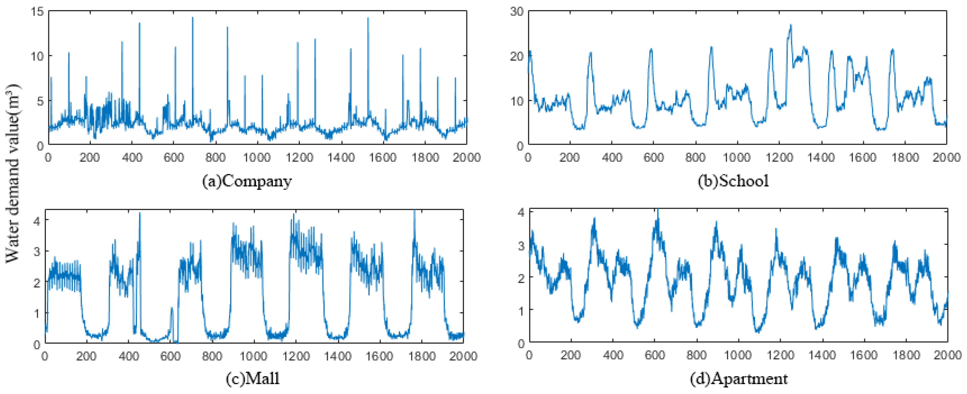
The experimental data in this paper were derived from the historical water demand dataset of a real-world water distribution system. As shown in Table 1, they are from four different types of areas, including commercial centers, universities, large malls, and residential areas, named as Company, School, Mall, and Apartment, respectively. Each dataset consists of seven channels of data, with each channel representing the flow data collected from flow sensors at different locations. The sampling interval is 5 min, and the time span is 1 year, totaling 105,120 water demand data points. In Figure 5, the waveform characteristics of the four datasets are distinctly represented. The Company dataset primarily exhibits a moderate oscillation with sporadic pulse-like waveforms, signaling abrupt alterations. The School dataset demonstrates a higher amplitude of fluctuation, accompanied by notable nonlinear attributes. The Mall dataset exhibits strong periodicity with waveforms akin to a square wave, yet it shows some fluctuation at the peak magnitudes. The Apartment dataset has a general periodic pattern, but it is subject to sharp variations within a single cycle’s duration. One month of data, totaling 8640 data points, was extracted for experimentation to validate the model’s performance under small sample sizes. The datasets were partitioned into three distinct subsets: a training set, a verification set, and a test set, following the ratio of 7:1:2, respectively. The linear interpolation method was used to process missing data:
W ( X ) = X X 1 Y 2 Y 1 X 2 X 1 + Y 1
where X is the target value, W ( X ) represents the target water demand, and (X1, Y1) and (X2, Y2) are adjacent data points of the target value.

3.1.2. Evaluation Metrics

In this study, we employed three distinct error assessment metrics—mean squared error (MSE), mean absolute error (MAE), and the coefficient of determination ( R 2 )—to evaluate the long-term forecasting accuracy of our model. The mathematical formulations of these metrics are delineated as follows:
MSE = 1 N i = 1 N Truth i Pred i 2 MAE = 1 N i = 1 N | Truth i Pred i R 2 = 1 i = 1 N Truth i Pred i 2 i = 1 N Truth i Truth ¯ 2
where N represents the length of the forecasting sequence, Truth i represents the actual water demand at time point i, Truth ¯ represents the average of the actual water demand, and Pred i represents the model’s forecast water demand at time point i. The smaller the value of the evaluation metric, the higher the accuracy of the model’s forecasts.

3.2. Results and Discussion

The model proposed in this paper was compared with long-term forecasting models, including Informer, Autoformer, FEDformer, DLiner, and SCINet [31]. In the fine-tuning processes of all the models, the Adam optimizer was employed. As shown in Table 2, the performance was compared across four types of datasets, with each consisting of 8640 water demand data points. The forecasting lengths of these models ranged from 48 to 720.
The experimental results presented in Table 2 illustrate that the proposed WDF-mixer model achieved the optimal predictive performance on the small-scale datasets, whereas DLinear and SCInet exhibited suboptimal predictive performance at varying forecasting lengths. Despite DLiner and SCINet’s relatively accurate predictions for the majority of data points, indicated by lower MSE and MAE scores, the impact of a small number of data points with larger errors is evident in the diminished R 2 score. SCInet utilized a recursive downsampling technique to decompose sequences for interactive learning, thereby enhancing the time series data and yielding satisfactory predictive outcomes. Meanwhile, DLinear decomposed time series into trend and residual components, employing two simplistic linear networks for modeling, also achieving satisfactory predictive performance. A comparative analysis of the methodological principles between the SCInet and DLinear models allowed us to derive the following conclusions [32,33]: (1) Decomposing sequences to address the low-rank characteristics of time series data can, to a certain extent, extract crucial features, facilitating easier modeling and representation of the data. (2) Due to the inherent low-rank nature of time series, decomposed sequences require only simple feature extraction methods to extract crucial information, resulting in favorable forecasting outcomes. These experimental observations further underscore the scientific rigor and effectiveness of the proposed time feature extraction module within the WDF-mixer framework. Notably, when contrasted with previous state-of-the-art outcomes, WDF-mixer achieved an average mean squared error (MSE) reduction of 25.02% in the Company dataset, 73.41% in the School dataset, 72.48% in the Mall dataset, and 79.53% in the Apartment dataset.
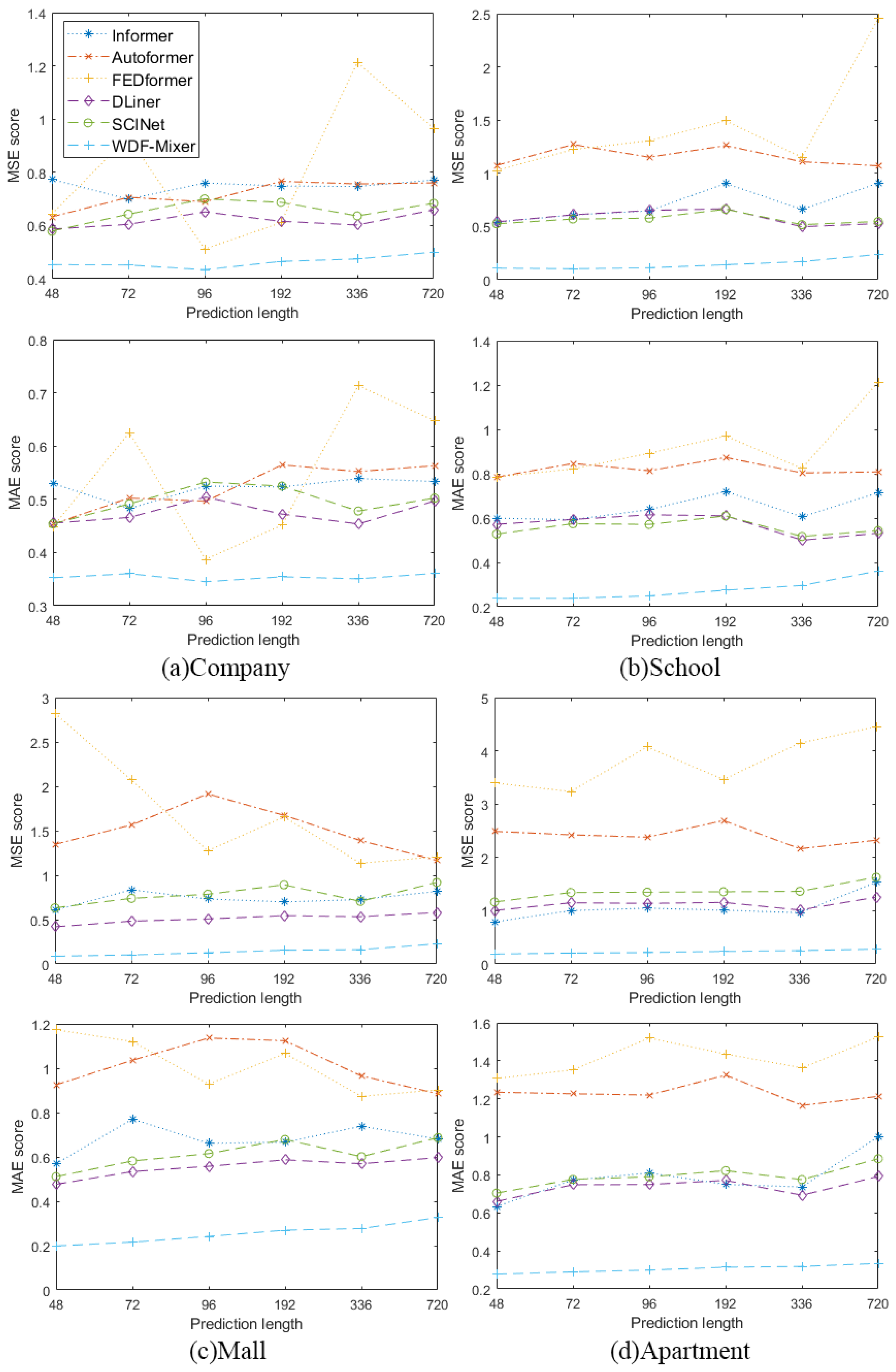
Figure 6 gives the metrics of the six forecasting models relative to the different samples. Along with the increase in forecasting length, the accuracy of the comparative models decreased. This result of the forecasting performance measure can be attributed to the change in correlation between the predictive sequence and the input sequence. Moreover, some characteristics did not only exist in one scale, but also in other scales. Hence, the forecasting performance might be poor if the features of the other scales were not considered. In contrast, the error curve of the WDF-mixer model consistently remained at the lowest position, which demonstrates the superiority of the model in long-term water demand forecasting. These results sufficiently illustrate that the WDF-mixer model has an advantage over comparative models in that it can represent long-range dependencies between observations. In addition, the data augmentation method, WGAN-GP, mitigates the impact of overfitting in water demand forecasting tasks that involve nonstationary series.
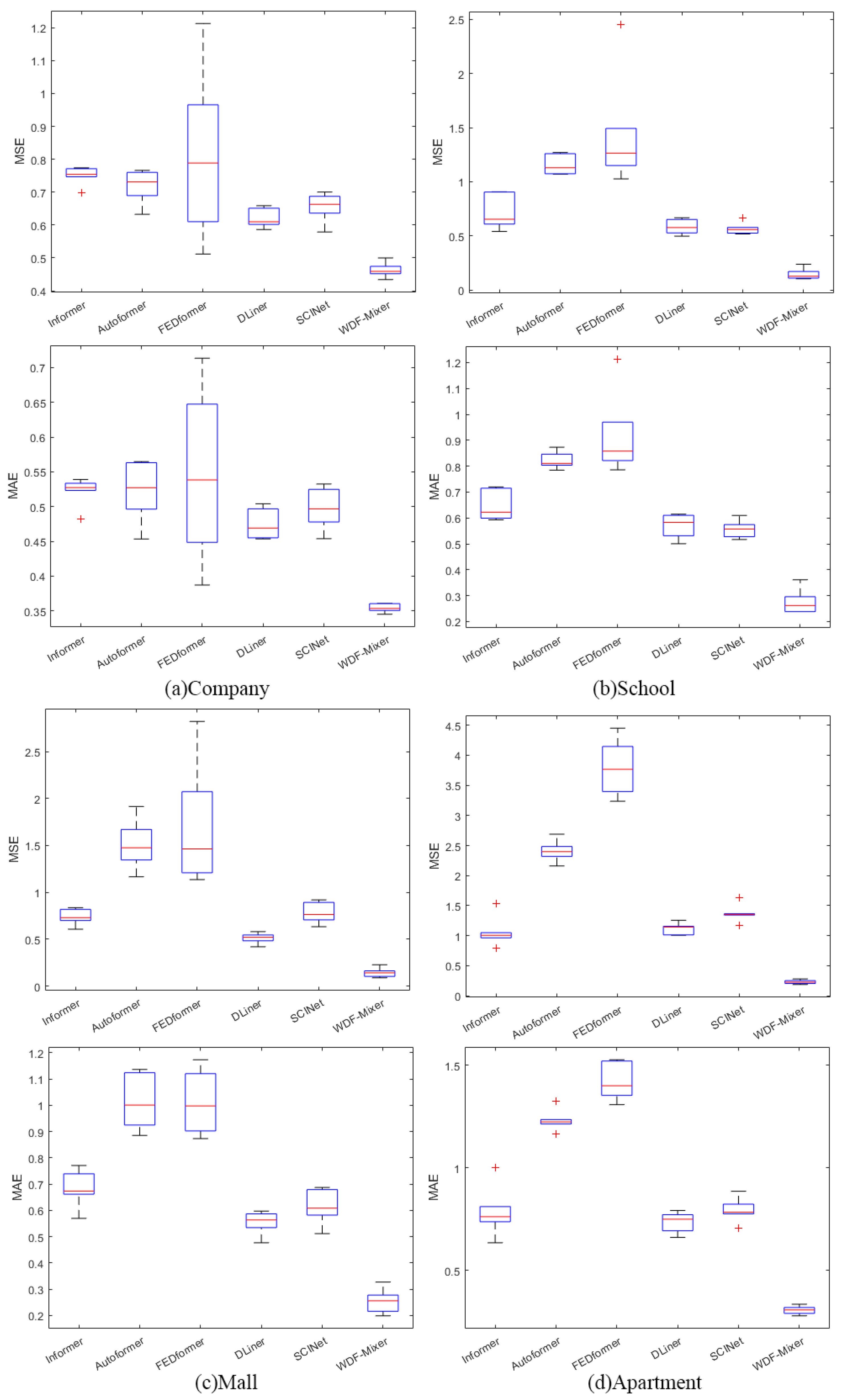
To assess the performance stability of all the algorithms, 50 independent experiments on four types of datasets were considered, and the results are shown in Figure 7. Compared to the other methods, the median and the interquartile of the WDF-mixer model remained at the lowest position in the graph, indicating high accuracy and robustness. These improvements achieved by the WDF-mixer model can be attributed to the multi-feature fusion. As such, diversity features can be utilized to improve predictive performance.

3.3. Ablation Study

In order to gain a better understanding of the proposed model’s behavior, this paper performed ablation studies on the WDF-mixer model, which mainly consisted of three parts: (1) the predictive performance of WDF-mixer variants; (2) the predictive effectiveness of multi-feature fusion; (3) the effectiveness of the data augmentation layer in small sample forecasting.
The variants of the WDF-mixer were named as “WDF-Mixer (enhanced functionality)”. The enhanced functionality represented either a single-channel feature extraction module (C), a data augmentation layer (E) or a combination of any of those terms. The following variants were compared:
WDF-mixer (none): Using only a temporal feature extraction module for forecasting.
WDF-mixer (C): Using a combination of temporal feature extraction module and channel feature extraction module forecasting.
WDF-mixer (E): Using a data augmentation layer for data expansion and a temporal feature extraction module for forecasting.
WDF-mixer (C,E): Using a data augmentation layer for data expansion and multi-dimensional feature fusion for forecasting.
Table 3 summarizes the performance of the four model variants on the real dataset. It is worth noting that in the first three datasets the WDF-mixer (C) model, which used multi-feature fusion, slightly outperformed the WDF-mixer (none) model. This was due to the Apartment’s nonlinearity being weaker than the others. The WDF-mixer (none) model already exhibited overfitting during forecasting. Therefore, when using the WDF-mixer (C) model with stronger nonlinear modeling capabilities, its forecasting error did not decrease but instead increased, exacerbating the overfitting problem.
Similarly, experiments were conducted on the Apartment dataset using the WDF-mixer (E) model. According to the experimental results, by adding a data augmentation layer to expand the sample data, the forecasting accuracy improved, indicating that data augmentation can effectively alleviate the model’s overfitting phenomenon. Furthermore, the WDF-mixer (C,E) model, after data augmentation, performed the best when using multi-feature fusion for feature extraction. It can be seen that the model’s data augmentation layer generated more meaningful sequence samples, enriching the features of the samples and significantly improving the forecasting accuracy.

4. Conclusions

Complex water demand patterns are formed during the process of urban development and are mainly affected by human activities. This study proposed a framework to delineate and analyze long-term water demand patterns and dynamics by using multi-feature fusion. The stability and superiority of the proposed model were verified through the experimental analysis of the proposed framework in real-world datasets.
In this study, a WGAN-BP method was used to generate synthetic data that resembled and complemented the original samples. And a gradient constraint was introduced to WGAN-BP, ensuring that the distribution of each parameter was uniform. Then, the obtained samples were decomposed into sub-sequences. For each sub-sequence, multiple MLP models were used for temporal feature extraction. In addition, a channel feature extraction module, based on the “Hamburger” structure, was used to avoid the risk of overfitting. Finally, an attention layer was used to capture depth characteristics and to obtain the temporal dependencies of the water demand.
This study presented the analysis of long-term water demand forecasting, taking advantage of big data sources from a smart water distribution system. This work should be helpful for the sustainable development and management of cities. In our future work, a more efficient forecasting method will be researched, and model interpretability could be considered.

Author Contributions

Conceptualization, C.Y.; funding acquisition, B.L. and Z.W.; methodology, J.M. and K.W.; software, J.M.; formal analysis, C.Y., B.L., Z.W. and K.W.; writing—original draft preparation, C.Y., J.M. and K.W. All authors have read and agreed to the published version of the manuscript.

Funding

This research was funded by the Zhejiang Provincial Natural Science Foundation of China No. LQ23F030002, the “Ling Yan” Research and Development Project of Science and Technology Department of Zhejiang Province of China under Grant Nos. 2022C03122, 2023C03161, and Public Welfare Technology Application and Research Projects of Zhejiang Province of China under Grant No. LGF22F020006.

Data Availability Statement

The data presented in this study are available on request from the corresponding author.

Acknowledgments

We would like to thank the editor and the reviewers for their kind help in improving this manuscript.

Conflicts of Interest

The authors declare no conflicts of interest.

References

  1. Fu, G.; Jin, Y.; Sun, S.; Yuan, Z.; Butler, D. The role of deep learning in urban water management: A critical review. Water Res. 2022, 223, 118973. [Google Scholar] [CrossRef]
  2. Chen, L.; Yan, H.; Yan, J.; Wang, J.; Tao, T.; Xin, K.; Li, S.; Pu, Z.; Qiu, J. Short-term water demand forecast based on automatic feature extraction by one-dimensional convolution. J. Hydrol. 2022, 606, 127440. [Google Scholar] [CrossRef]
  3. Zubaidi, S.L.; Hashim, K.; Ethaib, S.; Al-Bdairi, N.S.S.; Al-Bugharbee, H.; Gharghan, S.K. A novel methodology to predict monthly municipal water demand based on weather variables scenario. J. King Saud-Univ.-Eng. Sci. 2022, 34, 163–169. [Google Scholar] [CrossRef]
  4. Du, B.; Huang, S.; Guo, J.; Tang, H.; Wang, L.; Zhou, S. Interval forecasting for urban water demand using PSO optimized KDE distribution and LSTM neural networks. Appl. Soft Comput. 2022, 122, 108875. [Google Scholar] [CrossRef]
  5. Mokhtar, A.; Elbeltagi, A.; Gyasi-Agyei, Y.; Al-Ansari, N.; Abdel-Fattah, M.K. Prediction of irrigation water quality indices based on machine learning and regression models. Appl. Water Sci. 2022, 12, 76. [Google Scholar] [CrossRef]
  6. Stańczyk, J.; Kajewska-Szkudlarek, J.; Lipiński, P.; Rychlikowski, P. Improving short-term water demand forecasting using evolutionary algorithms. Sci. Rep. 2022, 12, 13522. [Google Scholar] [CrossRef]
  7. Pandey, P.; Bokde, N.D.; Dongre, S.; Gupta, R. Hybrid models for water demand forecasting. J. Water Resour. Plan. Manag. 2021, 147, 04020106. [Google Scholar] [CrossRef]
  8. Niknam, A.; Zare, H.K.; Hosseininasab, H.; Mostafaeipour, A.; Herrera, M. A critical review of short-term water demand forecasting tools—What method should I use? Sustainability 2022, 14, 5412. [Google Scholar] [CrossRef]
  9. Liu, X.; Zhang, Y.; Zhang, Q. Comparison of EEMD-ARIMA, EEMD-BP and EEMD-SVM algorithms for predicting the hourly urban water consumption. J. Hydroinform. 2022, 24, 535–558. [Google Scholar] [CrossRef]
  10. Li, H.; Wang, X.; Guo, H. Uncertain time series forecasting method for the water demand prediction in Beijing. Water Supply 2022, 22, 3254–3270. [Google Scholar] [CrossRef]
  11. Zubaidi, S.L.; Al-Bdairi, N.S.S.; Ortega-Martorell, S.; Ridha, H.M.; Al-Ansari, N.; Al-Bugharbee, H.; Hashim, K.; Gharghan, S.K. Assessing the benefits of nature-inspired algorithms for the parameterization of ANN in the prediction of water demand. J. Water Resour. Plan. Manag. 2023, 149, 04022075. [Google Scholar] [CrossRef]
  12. Huang, H.; Lin, Z.; Liu, S.; Zhang, Z. A neural network approach for short-term water demand forecasting based on a sparse autoencoder. J. Hydroinform. 2023, 25, 70–84. [Google Scholar] [CrossRef]
  13. Zanfei, A.; Brentan, B.M.; Menapace, A.; Righetti, M.; Herrera, M. Graph convolutional recurrent neural networks for water demand forecasting. Water Resour. Res. 2022, 58, e2022WR032299. [Google Scholar] [CrossRef]
  14. Rustam, F.; Ishaq, A.; Kokab, S.T.; de la Torre Diez, I.; Mazón, J.L.V.; Rodríguez, C.L.; Ashraf, I. An artificial neural network model for water quality and water consumption prediction. Water 2022, 14, 3359. [Google Scholar] [CrossRef]
  15. Guo, J.; Sun, H.; Du, B. Multivariable time series forecasting for urban water demand based on temporal convolutional network combining random forest feature selection and discrete wavelet transform. Water Resour. Manag. 2022, 36, 3385–3400. [Google Scholar] [CrossRef]
  16. Zhou, H.; Zhang, S.; Peng, J.; Zhang, S.; Li, J.; Xiong, H.; Zhang, W. Informer: Beyond efficient transformer for long sequence time-series forecasting. In Proceedings of the AAAI Conference on Artificial Intelligence, Virtual, 2–9 February 2021; Volume 35, pp. 11106–11115. [Google Scholar]
  17. Wu, H.; Xu, J.; Wang, J.; Long, M. Autoformer: Decomposition transformers with auto-correlation for long-term series forecasting. Adv. Neural Inf. Process. Syst. 2021, 34, 22419–22430. [Google Scholar]
  18. Zhou, T.; Ma, Z.; Wen, Q.; Wang, X.; Sun, L.; Jin, R. Fedformer: Frequency enhanced decomposed transformer for long-term series forecasting. In Proceedings of the International Conference on Machine Learning. PMLR, Baltimore, MD, USA, 17–23 July 2022; pp. 27268–27286. [Google Scholar]
  19. Zeng, A.; Chen, M.; Zhang, L.; Xu, Q. Are transformers effective for time series forecasting? In Proceedings of the AAAI Conference on Artificial Intelligence, Washington, DC, USA, 7–14 February 2023; Volume 37, pp. 11121–11128. [Google Scholar]
  20. Sheng, Z.; Wen, S.; Feng, Z.k.; Gong, J.; Shi, K.; Guo, Z.; Yang, Y.; Huang, T. A survey on data-driven runoff forecasting models based on neural networks. IEEE Trans. Emerg. Top. Comput. Intell. 2023, 7, 1083–1097. [Google Scholar] [CrossRef]
  21. Sheng, Z.; Wen, S.; Feng, Z.k.; Shi, K.; Huang, T. A Novel Residual Gated Recurrent Unit Framework for Runoff Forecasting. IEEE Internet Things J. 2023, 10, 12736–12748. [Google Scholar] [CrossRef]
  22. Zhang, C.; Sheng, Z.; Zhang, C.; Wen, S. Multi-lead-time short-term runoff forecasting based on Ensemble Attention Temporal Convolutional Network. Expert Syst. Appl. 2024, 243, 122935. [Google Scholar] [CrossRef]
  23. Geng, X.; He, X.; Xu, L.; Yu, J. Attention-based gating optimization network for multivariate time series prediction. Appl. Soft Comput. 2022, 126, 109275. [Google Scholar] [CrossRef]
  24. Iglesias, G.; Talavera, E.; González-Prieto, Á.; Mozo, A.; Gómez-Canaval, S. Data augmentation techniques in time series domain: A survey and taxonomy. Neural Comput. Appl. 2023, 35, 10123–10145. [Google Scholar] [CrossRef]
  25. Wang, H.; Zhang, Y.; Liang, J.; Liu, L. DAFA-BiLSTM: Deep autoregression feature augmented bidirectional LSTM network for time series prediction. Neural Netw. 2023, 157, 240–256. [Google Scholar] [CrossRef]
  26. Shangguan, A.; Xie, G.; Fei, R.; Mu, L.; Hei, X. Train wheel degradation generation and prediction based on the time series generation adversarial network. Reliab. Eng. Syst. Saf. 2023, 229, 108816. [Google Scholar] [CrossRef]
  27. Luleci, F.; Catbas, F.N.; Avci, O. Generative adversarial networks for labeled acceleration data augmentation for structural damage detection. J. Civ. Struct. Health Monit. 2023, 13, 181–198. [Google Scholar] [CrossRef]
  28. Pérez, J.; Arroba, P.; Moya, J.M. Data augmentation through multivariate scenario forecasting in Data Centers using Generative Adversarial Networks. Appl. Intell. 2023, 53, 1469–1486. [Google Scholar] [CrossRef]
  29. Demir, S.; Mincev, K.; Kok, K.; Paterakis, N.G. Data augmentation for time series regression: Applying transformations, autoencoders and adversarial networks to electricity price forecasting. Appl. Energy 2021, 304, 117695. [Google Scholar] [CrossRef]
  30. Geng, Z.; Guo, M.H.; Chen, H.; Li, X.; Wei, K.; Lin, Z. Is attention better than matrix decomposition? arXiv 2021, arXiv:2109.04553. [Google Scholar]
  31. Liu, M.; Zeng, A.; Chen, M.; Xu, Z.; Lai, Q.; Ma, L.; Xu, Q. Scinet: Time series modeling and forecasting with sample convolution and interaction. Adv. Neural Inf. Process. Syst. 2022, 35, 5816–5828. [Google Scholar]
  32. Chen, Z.; Ma, M.; Li, T.; Wang, H.; Li, C. Long sequence time-series forecasting with deep learning: A survey. Inf. Fusion 2023, 97, 101819. [Google Scholar] [CrossRef]
  33. Sousa, J.; Henriques, R. Intersecting reinforcement learning and deep factor methods for optimizing locality and globality in forecasting: A review. Eng. Appl. Artif. Intell. 2024, 133, 108082. [Google Scholar] [CrossRef]
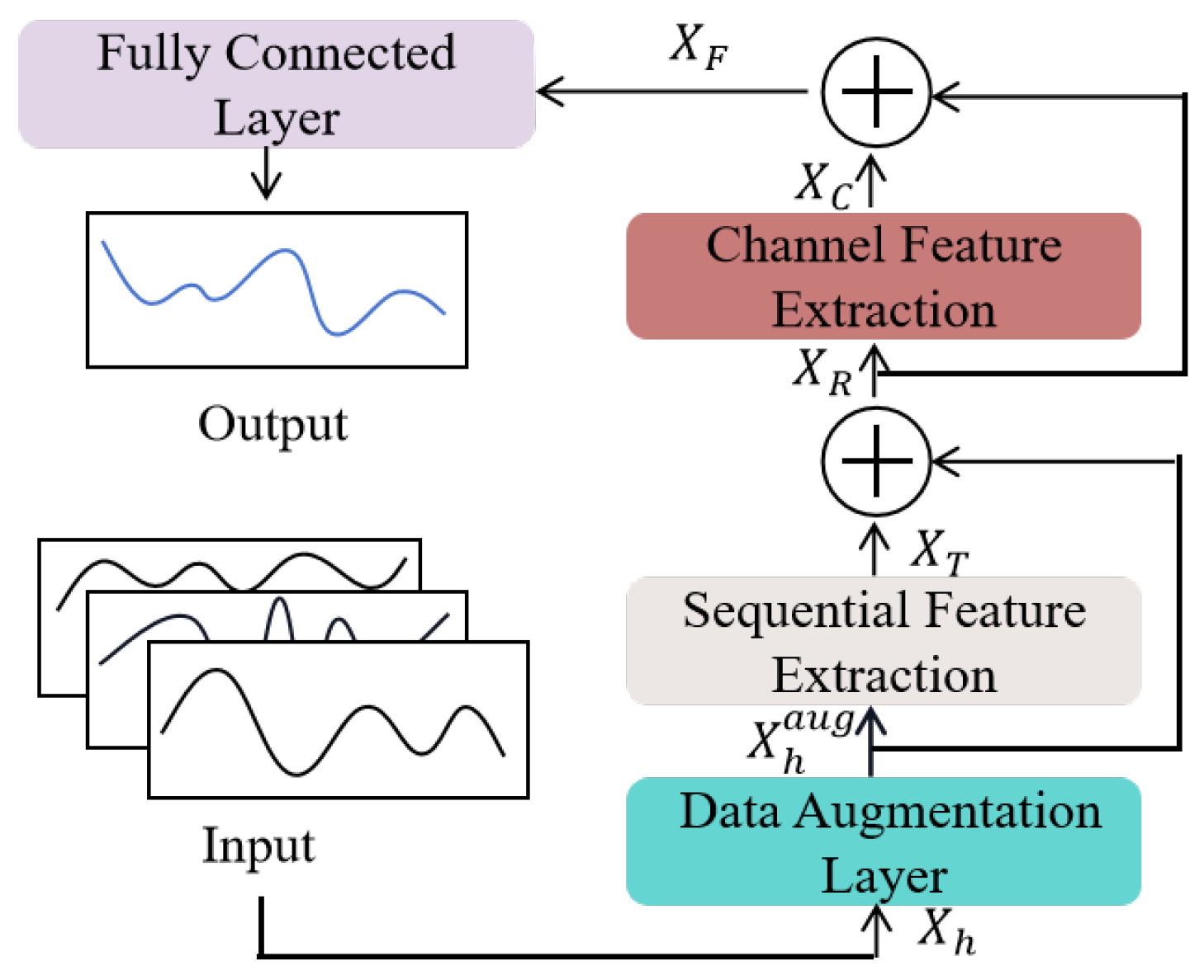
Figure 1. The overall architecture diagram of the WDF-mixer.
Water 16 01731 g001
Figure 2. Schematic diagram of WGAN-GP data enhancement layer network structure.
Water 16 01731 g002
Figure 3. Module structure diagram of sequential feature extraction.
Water 16 01731 g003
Figure 4. Module structure diagram of channel feature extraction.
Water 16 01731 g004
Figure 5. The water demand across four different datasets, with 2000 samples per dataset (the x-axis corresponds to the sample point number and the y-axis to the water demand value).
Water 16 01731 g005
Figure 6. Error score polygons for different water demand datasets, illustrating the performance of various models over a range of forecasting lengths.
Water 16 01731 g006
Figure 7. Box-line diagram of forecasting errors of different models for four types of water demand datasets. (“+” represents as the outlier).
Water 16 01731 g007
Table 1. Overview of the experimental datasets.
The Name of the DatasetData SourcesNumber of ChannelsTotal Amount of Data
CompanyThe city’s commercial center.7105,120
SchoolUniversities in the city.7105,120
MallThe city malls.7105,120
ApartmentResidential areas of the city.7105,120
Table 2. Time series error scores for predicting water demand in four distinct datasets, all initialized with an input length of 96 and extending to output lengths of 48, 72, 96, 192, 336, and 720. The best-performing results are displayed in bold, and near-optimal results are underscored.
ModelsInformerAutoformerFEDformer
MetricMSEMAE R 2 MSEMAE R 2 MSEMAE R 2
Company480.77390.52980.34720.63250.45340.13310.64340.44850.4022
720.69870.48270.30780.70600.50240.37650.93380.62520.4085
960.75990.52480.30880.68960.49630.28430.51180.38720.2571
1920.74830.52320.06430.76600.56470.28380.61020.45150.4025
3360.74660.53890.27520.75630.55210.14611.21260.71350.4127
7200.77130.5335−0.00060.76010.56320.29570.96540.6474−0.0401
School480.54160.59910.55691.07450.78470.01011.02660.78590.1506
720.60900.59260.34781.27060.8463−0.17951.22340.82150.0198
960.64790.63870.57321.15090.81330.05671.30610.8922−0.0949
1920.90560.71980.28101.26050.8732−0.17831.49360.9700−0.0840
3360.66030.60600.42731.10840.80370.07031.14980.82410.0122
7200.90770.71470.12811.07090.80810.02452.45511.21350.0367
Mall480.60600.56940.71001.34580.9247−0.06202.82191.17300.0193
720.83610.77040.52441.56401.03590.03222.07161.1201−0.3236
960.73270.66140.47321.91321.1360−0.26401.27370.9279−0.0661
1920.69980.66620.52221.67171.1238−0.36951.65391.0669−0.0341
3360.72660.73870.18521.38900.9653−0.20761.13640.87310.0684
7200.81820.68060.23061.16640.8849−0.36941.20840.9022−0.1449
Apartment480.79170.63390.59662.48581.2347−0.18413.39571.30730.1156
721.00330.77270.67122.42191.2265−0.14873.23441.35230.0530
961.04950.81050.57592.37671.2201−0.25714.07191.5199−0.2556
1921.01010.75000.66022.69001.3247−0.28483.46081.4361−0.0409
3360.96500.73660.57402.16081.1653−0.09474.14601.36300.1820
7201.53411.00180.47502.32091.2129−0.03874.45061.5262−0.0281
ModelsDLinerSCINetWDF-Mixer
MetricMSEMAE R 2 MSEMAE R 2 MSEMAE R 2
Company480.58640.45510.20150.57890.45390.22790.45280.35260.4575
720.60430.46590.17480.64260.49130.13410.45190.36040.4582
960.65120.50410.10330.70020.53240.06800.43410.34510.4613
1920.61580.47220.15260.68730.52480.05010.46510.35440.4449
3360.60190.45360.19160.63620.47790.14680.47430.35060.4400
7200.65880.49680.11880.68340.50230.10410.49990.36090.4103
School480.54370.57200.36920.52530.52780.39050.10990.23840.8826
720.61060.59370.29150.57050.57440.33800.10410.23840.8884
960.65150.61470.24810.57850.57120.33240.11330.24940.8781
1920.66700.61010.26300.66200.60960.26850.14150.27480.8496
3360.49770.50040.44820.51740.51700.24630.17090.29620.8203
7200.52750.53140.40710.54770.54390.38440.23770.36160.7490
Mall480.41880.47640.46600.63360.51120.19210.08760.19840.8999
720.48280.53390.36190.74000.58150.02190.10290.21570.8815
960.50760.55780.31790.78640.6148−0.05670.12680.24160.8532
1920.54470.58660.25000.89270.6788−0.22920.15490.26960.8175
3360.53310.56910.25140.70620.60110.00850.16210.27710.8042
7200.58090.59680.15810.91930.6869−0.33240.22710.32680.7161
Apartment481.00600.66050.32891.16480.70410.22300.18700.27800.8458
721.14990.74830.21851.34340.77640.08690.20460.29000.8299
961.13890.74950.21431.34910.78980.06930.21580.29910.8194
1921.15640.77100.19701.35700.82240.05770.23630.31440.8024
3361.01380.69260.31161.36560.77520.07270.25140.31840.7920
7201.25610.79160.17071.63070.8850−0.07650.27930.33420.7721
Table 3. MSE score table of ablation results (the input length was 96 and the output length was 48, 72, 96, 192, 336, 720, respectively. The best results are highlighted in bold, and the suboptimal results are highlighted with an underscore).
DatasetFLWDF-mixer
(None)
WDF-mixer
(C)
WDF-mixer
(E)
WDF-mixer
(C,E)
Company480.63870.58180.48800.4528
720.65010.65330.50170.4519
960.63150.59930.51540.4341
1920.65090.63050.54000.4651
3360.61800.61800.54520.4743
7200.68410.67900.58890.4999
School480.28820.30980.16710.1099
720.38090.34650.15460.1041
960.37250.34090.16190.1133
1920.41440.34260.20960.1415
3360.32930.32530.21760.1709
7200.44390.41470.30320.2377
Mall481.11140.71980.19810.0876
721.02800.92360.20310.1029
961.50541.30830.23490.1268
1921.19781.01260.24600.1549
3360.99211.16550.22380.1621
7201.03100.91600.29960.2271
Apartment482.97853.40510.23180.1870
723.19283.50350.27210.2046
963.45043.68430.28740.2158
1922.93783.55520.31530.2363
3362.47872.24050.30390.2514
7203.50424.14760.34210.2793
Improvement over WDF-mixer2.48%58.24%67.14%
Disclaimer/Publisher’s Note: The statements, opinions and data contained in all publications are solely those of the individual author(s) and contributor(s) and not of MDPI and/or the editor(s). MDPI and/or the editor(s) disclaim responsibility for any injury to people or property resulting from any ideas, methods, instructions or products referred to in the content.