Abstract
This study evaluates the performance of Global Climate Models (GCMs) in simulating extreme climate in three northeastern provinces of China (TNPC). A total of 23 GCMs from the Coupled Model Intercomparison Project Phase 6 (CMIP6) were selected and compared with observations from 1961 to 2010, using the 12 extreme climate indices defined by the Expert Team on Climate Change Detection and Indicators. The Interannual Variability Skill Score (IVS), Taylor diagrams and Taylor Skill Scores (S) were used as evaluation tools to compare the outputs of these 23 GCMs with the observations. The results show that the monthly minimum of daily minimum temperature (TNn) is overestimated in 55.7% of the regional grids, while the percentage of time when the daily minimum temperature is below the 10th percentile (TN10p) and the monthly mean difference between the daily maximum and minimum temperatures (DTR) are underestimated in more than 95% of the regional grids. The monthly maximum value of the daily maximum temperature (TXx) and the annual count when there are at least six consecutive days of the minimum temperature below the 10th percentile (CSDI) have relatively low regional spatial biases of 1.17 °C and 1.91 d, respectively. However, the regional spatial bias of annual count when the daily minimum temperature is below 0 °C (FD) is relatively high at 9 d. The GCMs can efficiently capture temporal variations in CSDI and TN10p (IVS < 0.5), as well as the spatial patterns of TNn and FD (S > 0.8). For the extreme precipitation indices, GCMs overestimate the annual total precipitation from days greater than the 95th percentile (R95p) and the annual count when precipitation is greater than or equal to 10 mm (R10 mm) in more than 90% of the regional grids. The maximum number of consecutive days when precipitation is below 1 mm (CDD) and the ratio of annual total precipitation to the number of wet days (greater than or equal to 1 mm) (SDII) are underestimated in more than 80% and 54% of the regional grids, respectively. The regional spatial bias of the monthly maximum consecutive 5-day precipitation (RX5day) is relatively small at 10.66%. GCMs are able to better capture temporal variations in the monthly maximum 1-day precipitation (RX1day) and SDII (IVS < 0.6), as well as spatial patterns in R95p and R10mm (S > 0.7). The findings of this study can provide a reference that can inform climate hazard risk management and mitigation strategies for the TNPC.
1. Introduction
With global warming, the intensity and frequency of extreme climate events have increased [1,2], resulting in far-reaching impacts on human societies and natural ecosystems [3]. For instance, California experienced a record temperature of 54.4 °C on 9 July 2021—it was the hottest summer on record averaged over the continental United States—and the city of Zhengzhou, a one-hour rainfall of 201.9 mm on 20 July 2021, which led to flooding and caused more than 302 deaths and USD 17.7 billion in economic losses in China [4]. It is worth noting that even relatively small incremental increases in global warming (+0.5 °C) can cause statistically significant changes in extreme climate on a global scale and over large regions [5]. Therefore, it is critical to study extreme climate and develop effective adaptation strategies.
Due to the complexity of extreme climate, projecting extreme climate events remains a recognized challenge [6,7,8]. GCMs are by far the most effective tool for simulating past and future climate [9]. At present, the Coupled Model Intercomparison Project has developed into the sixth phase (CMIP6) [10,11]. CMIP6 GCMs have significantly improved the capability of simulating climate change at global and regional scales [12], which could better simulate extreme climate [13,14]. Compared to older versions of CMIP, CMIP6 has higher spatial resolution, incorporates new physical processes and biogeochemical cycles, thereby contributing to a more accurate representation of key feedback mechanisms affecting climate change [15,16]. These improvements enhance the performance of GCMs in historical simulation and future projection. Nevertheless, several studies [8,15,17] have shown that despite the general improvement in the capacity of CMIP6 GCMs to simulate extreme climate, they are still constrained in regions with complex topographic [18] and climatic conditions [19]. Therefore, it is important to evaluate the study of GCMs in these regions.
As an important grain-producing area in China, the three northeastern provinces of China (TNPC) region has been continuously influenced by extreme high temperature, drought, flood, and other catastrophic climate events over the past few years [20,21,22]. The region has been significantly affected by these disasters, with serious consequences for both its socio-economic development and the well-being of its residents. Moreover, TNPC is located in the mid–high latitude region, with high fluctuations in temperature and precipitation [23], which makes it highly susceptible to extreme climate events. However, there are few studies of the capacity to simulate extreme climate in this region [9,24].
As a result, this study evaluates the performance of CMIP6 GCMs in simulating extreme temperature and extreme precipitation through Interannual Variability Skill Score (IVS), Taylor diagrams and Taylor Skill Scores (S) using observations and GCMs outputs from the TNPC region from 1961 to 2010. The results of this study can provide a valuable reference for anticipating and mitigating extreme climate in this region.
2. Materials and Methods
2.1. Study Area
TNPC (118° E–135° E, 48° N–55° N) is located in the northeastern part of China and includes the Heilongjiang, Jilin, and Liaoning Provinces, with a total area of 787,300 km2 (Figure 1). There are significant climate differences between internal regions, with average annual temperatures ranging from 2.75 to 5.72 °C and average annual precipitation ranging from 400 to 800 mm. The topography of TNPC is complex, characterized by a combination of plains, mountains, and numerous river systems. The Xiaoxing’an Mountains are located in the east, the Changbai Mountain Range is in the southeast, and the Northeast Plain, which is China’s largest plain, lies at the center. TNPC is also surrounded by rivers such as the Heilong Jiang and the Ussuri River. This region is an important base for the production of commercial grain in China, and the distribution of temperature and precipitation is uneven with obvious interannual fluctuations. Grain production is greatly affected by extreme climate events.
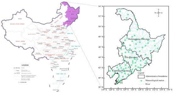
Figure 1.
Overview of the study area.
2.2. Data
The observations used in this study include three variables, precipitation, daily maximum temperature and daily minimum temperature, provided by the China Meteorological Data Network (http://data.cma.cn (accessed on 6 May 2023)) based on 86 stations located in the study area. The dataset was subjected to a strict quality control process and is widely used [25,26]. For missing values of one or two days, we used the average of adjacent days instead. For missing values that exceeded two days, we applied interpolation based on the multi-year average of the same day from other years [27].
This study used the simulated temperature and precipitation data from 23 CMIP6 models (Table 1) provided by the Earth System Grid Federation (https://esgf-node.llnl.gov/projects/esgf-llnl/ (accessed on 6 May 2023)), with the study period being from 1961 to 2010.

Table 1.
Basic information of the 23 CMIP6 GCMs.
Distance inverse interpolation and bilinear interpolation were used to interpolate the observations and the outputs of the selected GCMs into 418 grids of 50 km × 50 km resolution. These two interpolation methods are common approaches used for interpolation [28,29].
2.3. Extreme Climate Indices
Here, we focus on the 12 extreme climate indices defined by the Expert Team on Climate Change Detection and Indicators (Table 2) [30]. These indices represent the frequency, intensity, or duration of extreme climate events over a specific time period and are widely used in extreme climate study [7,31,32,33].
Table 2.
Definitions of extreme climate indices.
2.4. Evaluation Methods
2.4.1. Biases
We used the mean bias (MB) and mean relative bias (MRB) to evaluate the performance of the GCMs in simulating extreme temperature and extreme precipitation, respectively. However, R10mm and CDD in the extreme precipitation indices were evaluated using MB. Since the mean values could be highly influenced by a few abnormal values, the median is employed to display the ensemble of 23 CMIP6 models. The absolute regional spatial bias was obtained by calculating the median spatial bias of the 23 GCMs in each grid, accumulating the absolute values of these median values across all grids, and then averaging this cumulative result:
where and represent the average values of the GCMs outputs from 1961 to 2010, and represent the average values of observations from 1961 to 2010, and n and i represent extreme indices.
2.4.2. IVS
In this study, IVS was used to evaluate the temporal simulation capability of the CMIP6 GCMs [34]:
where STDm and STDo represent the standard deviation of the simulated and observations for each grid, respectively. A lower IVS indicates a stronger temporal simulation capability of the GCMs. The regional temporal simulation performance of the GCMs is obtained by weighting and averaging the IVS for all grid points.
2.4.3. Taylor Diagram and S
The regional spatial simulation performance of the GCMs was evaluated using Taylor diagram and S; the specific methodology is detailed in the literature [35]. The Taylor diagram provided a visual evaluation of the correlation coefficients (R), standard deviation ratios (σ), and root-mean-square errors (E′) between the GCMs outputs and the observations on a single figure. Among these indices, R represents the spatial correlation coefficient between observations and GCMs outputs, σ is the ratio of the spatial standard deviation of the GCMs outputs to that of the observations, and E′ indicates the average degree of deviation of the GCM from the observations [36]. The ideal simulation has E’ centered at 0, with both R and σ close to 1.
One of the least complicated scores S was used to evaluate the model’s regional simulation effectiveness, and was defined as shown in Equation (4):
where Rmax stands for the maximum value attainable for R. The spatial simulation performance of the GCMs is considered to be the best when the S is close to 1.
3. Results
3.1. Spatial Bias Analysis
3.1.1. Spatial Biases of Extreme Temperature Indices
The FD, TXx, TNn and CSDI of the multi-model median in the southwestern Heilongjiang and northwestern Jilin Provinces are similar to the observations (Figure 2). The FD, TXx and TNn of the multi-model median in most parts of Liaoning Province are also similar to the observations, except for the CSDI. Overall, the observations of both TN10p and DTR are higher than the multi-model median. The regional spatial biases of the FD, TXx, TNn, TN10p, CSDI and DTR are 9 d, 1.17 °C, 2.34 °C, 4.71 d, 1.91 d and 2.85 °C from 1961 to 2010, respectively (Figure 3, Figure 4, Figure 5, Figure 6, Figure 7 and Figure 8). The results indicate that the multi-model median can reproduce the spatial distributions of FD, TXx, TNn and CSDI in southwest Heilongjiang, northwest Jilin and northwest Liaoning Provinces, but performs poorly for the simulation of TN10p and DTR.
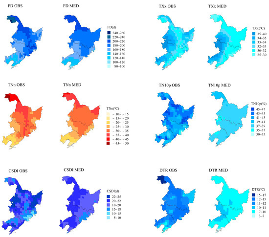
Figure 2.
The spatial distribution of observations and GCMs outputs (OBS represents observations and MED represents the median of 23 GCMs).
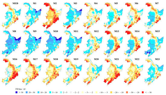
Figure 3.
The simulated biases of FD via 23 GCMs.
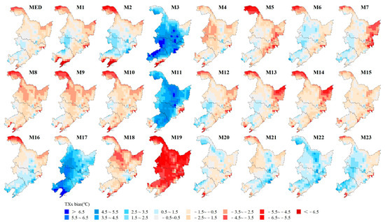
Figure 4.
The simulated biases of TXx via 23 GCMs.
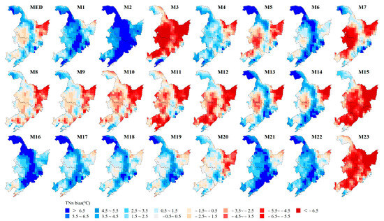
Figure 5.
The simulated biases of TNn via 23 GCMs.
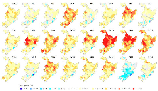
Figure 6.
The simulated biases of TN10p via 23 GCMs.
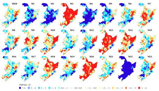
Figure 7.
The simulated biases of CSDI via 23 GCMs.
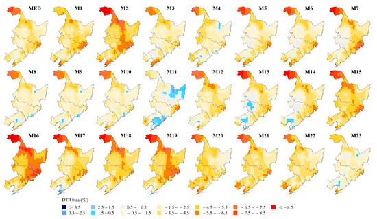
Figure 8.
The simulated biases of DTR via 23 GCMs.
From the MED, the multi-model median performs well in simulating TXx and CSDI, with spatial biases of ±3 °C and ±4 d, respectively. It is noteworthy that only TNn shows a positive bias in 55.7% of the regional grids, while the other indices show negative biases in more than half of the regional grids. In particular, TN10p and DTR have negative biases in more than 95% of the regional grids. These results indicate that GCMs may underestimate FD, TXx, TN10p, CSDI and DTR.
The spatial distributions of the TXx and TN10p indices are well simulated by nearly half of the GCMs, with M1, M7 and M16 simulating the spatial distribution of both indices better. The simulations of M3 and M11 for the TXx show positive biases of more than 1.5 °C, indicating that the simulated maximum temperature is more than 1.5 °C higher than the observations, resulting in an overestimation of the maximum temperature. When simulating the TN10p, M22 shows a considerable positive bias in the Jilin and Liaoning Provinces, indicating that the projected TN10p decreases 3–6 d. The simulation biases of FD, TNn and CSDI vary considerably among GCMs. In northern and central Heilongjiang Province and most regions of the Jilin and Liaoning Provinces, half of the GCMs simulations show a large negative bias in FD, while the TNn shows a significant positive bias. The CDSI simulated via M3 and M22 are opposite, with the M3 showing a negative bias while M22 shows a positive bias. Most GCMs consistently underestimate DTR. We also find that GCMs from the same organization have similar biases and ranges in spatial performance. For instance, M8, M9 and M10 from EC-Earth-Consortium all show similar simulation biases. In general, none of the GCMs accurately reproduce the spatial performance of six extreme temperature indices.
3.1.2. Spatial Biases of Extreme Precipitation Indices
The multi-model median for R95p and R10mm is higher than the observations in north-western and eastern Heilongjiang Province, northeastern Jilin Province and eastern Liaoning Province (Figure 9). For RX1day, the observations are higher than the multi-model median in southern Heilongjiang Province, northwestern Jilin Province and most of the Liaoning Province. For CDD, the observations in southwestern Heilongjiang Province, western Jilin Province, and southwestern Liaoning Province are higher than the multi-model median. As for the SDII, the regional observations are higher than the multi-model median. The regional spatial biases of the RX1day, RX5day, R95p, R10mm, CDD and SDII indices are 15.32%, 10.66%, 29.10%, 3.24d, 15.67d and 18.04% from 1961 to 2010, respectively (Figure 10, Figure 11, Figure 12, Figure 13, Figure 14 and Figure 15). The results show that there is a large bias between the observations and GCMs outputs in northern and southeastern Heilongjiang Province and northeastern Jilin Province.
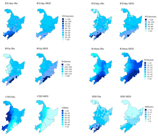
Figure 9.
The spatial distribution of observations and MED (OBS represents observations and MED represents the median of 23 GCMs).
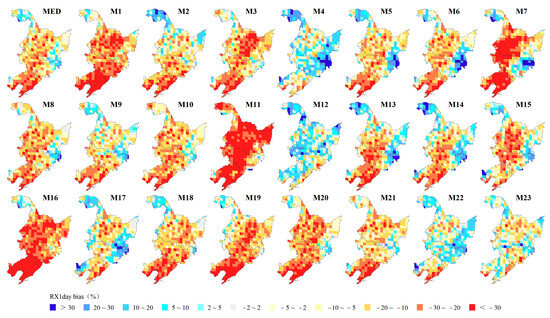
Figure 10.
The simulated biases of RX1day via 23 GCMs.
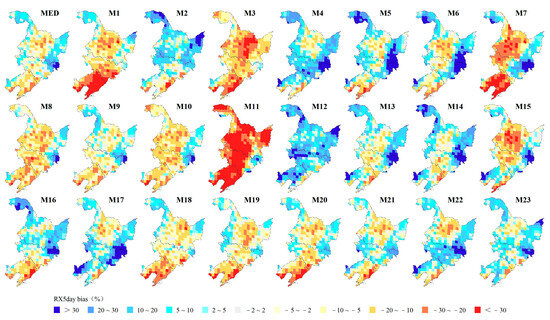
Figure 11.
The simulated biases of RX5day via 23 GCMs.
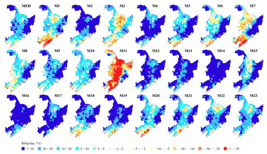
Figure 12.
The simulated biases of R95p via 23 GCMs.
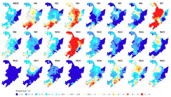
Figure 13.
The simulated biases of R10mm via 23 GCMs.
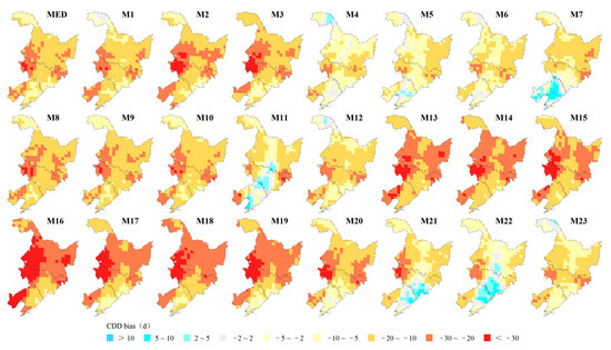
Figure 14.
The simulated biases of CDD via 23 GCMs.
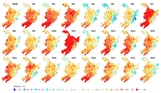
Figure 15.
The simulated biases of SDII via 23 GCMs.
Based on the MED, it can be seen that the multi-model median performs best for the RX5day, with spatial bias generally controlled within 10%, and worst for the R95p, with spatial bias at 29.10%. In more than 90% of the regional grids, the simulations of R95p and R10mm show positive biases, while the simulations of CDD and SDII have negative biases. In addition, the RX1day shows negative biases in exceeding 80% of the regional grids, and RX5day also has negative bias over 54% of the regional grids.
For RX1day, most of the GCMs show positive biases in the northern part of Heilongjiang Province, which overestimate the 1d maximum precipitation, and except for M4, M12, M17, M22 and M23, the other GCMs show negative biases in all regions except the northern part of Heilongjiang Province. For RX5day, R95p and R10mm, only M1, M3, M7 and M11 show significant negative biases over TNPC, and for R95p and R10mm, the other GCMs show great positive biases, especially in the southeastern part of Heilongjiang Province, where the positive biases are over 30% and 5d. For CDD and SDII, a vast number of GCMs have negative biases, underestimating the number of consecutive drought days and simple precipitation intensity index.
3.2. Temporal Simulation Capability
3.2.1. Temporal Simulation Capabilities of GCMs for Extreme Temperature Indices
All GCMs perform well in simulating the interannual variability of CSDI, with an IVS lower than 0.45, followed by TN10p, with an IVS lower than 0.63 (Figure 16). For interannual variability in FD, except M8 and M11, the other GCMs have an IVS within 0.25. However, most GCMs simulate the interannual variability of TXx and DTR poorly, with an IVS exceeding 1.0. It is noteworthy that the M15 has an excellent interannual variability performance for all indices, with an IVS below 0.58.
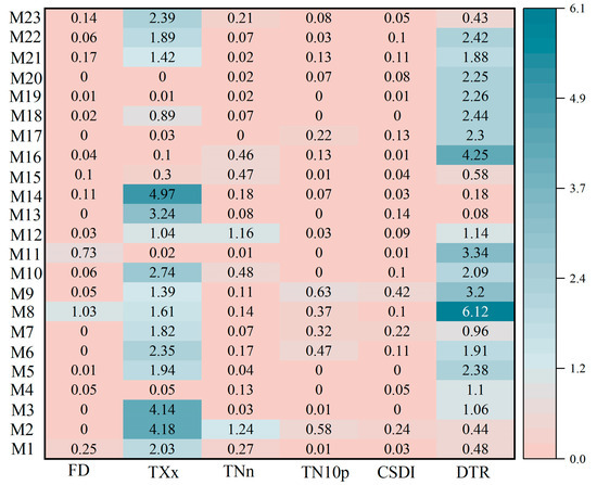
Figure 16.
Heat maps of the IVS in extreme temperature indices for 23 GCMs from 1961 to 2010 (the closer to the light pink color, the better the temporal simulation, the same meaning of the color in Figure 17, Figure 19 and Figure 20).
3.2.2. Temporal Simulation Capabilities of GCMs for Extreme Precipitation Indices
Compared to the temporal simulation capabilities of the extreme temperature indices, the GCMs can only simulate well the interannual variability of RX1day, with an IVS in the range of 0 to 0.65 (Figure 17). This is closely followed by SDII, which is only poorly simulated via M15, as the other GCMs have an IVS in the range of 0 to 0.6. More than half of the GCMs simulate RX5day and CDD well, but the interannual variability of R95p and R10mm is poorly simulated, with most of the GCMs having an IVS greater than 0.8. In terms of simulating the interannual variability of extreme precipitation, M1 and M10 perform the best, with an IVS below 0.36.
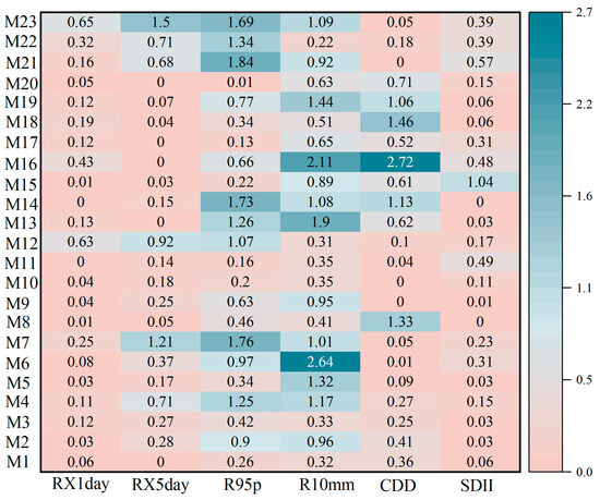
Figure 17.
Heat maps of the IVS in extreme precipitation indices for 23 GCMs from 1961 to 2010.
3.3. Spatial Simulation Capability
3.3.1. Spatial Simulation Capabilities of GCMs for Extreme Temperature Indices
The GCMs are the best at spatially simulating FD and TNn, with most of them having R above 0.85, σ close to 1, and E′ ranging between 0.25 and 0.75 (Figure 18). On the contrary, these seem to perform poorly in the simulation of TN10p and CSDI, with R below 0.20, σ close to 0.5, and E′ higher than 1. For TXx, the R ranges between 0.5 and 0.7, but the GCMs deviate considerably from the observations in terms of σ and E′. For DTR, most GCMs have σ between 0.6 and 0.8, and E′ below 1.25, indicating good spatial simulation performance, but the lower R (below 0.5) shows a relatively poor correlation compared to the other indices.
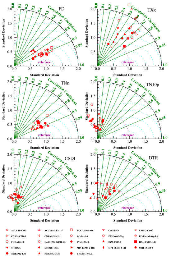
Figure 18.
The Taylor diagram of the spatial simulation capabilities of 23 GCMs for extreme temperature indices from 1961 to 2010.
The S of FD and TNn from CMIP6 GCMs are above 0.8 (Figure 19). In contrast, the spatial patterns of TN10p and CSDI perform poorly, with S below 0.5. The S of M5 and M9 all exceed 0.62, indicating that they perform well in spatially simulated extreme temperature indices, while M2, M17, M18 and M19 perform poorly.
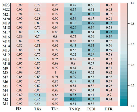
Figure 19.
Heat maps of the S in extreme temperature indices for 23 GCMs from 1961 to 2010.
3.3.2. Spatial Simulation Capabilities of GCMs for Extreme Precipitation Indices
The CDD has the highest R, close to 0.9, followed by RX1day and SDII, while R10mm performs relatively worse with R ranging from 0.2 to 0.8 (Figure 20). For R95p and R10mm, σ ranges from 0.8 to 1.2, while for RX1day, RX5day, CDD and SDII, σ is less than 0.8. The E’ for all indices ranges from 0.5 to 1. There are significant differences among the GCMs. For instance, M19 simulates R10mm best with R above 0.8, σ of 1, and E’ lower than 0.75, but it simulates the other indices poorly.
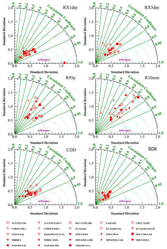
Figure 20.
The Taylor diagram of the spatial simulation capabilities of 23 GCMs for extreme precipitation indices from 1961 to 2010.
The spatial simulations of R95p and R10mm perform the best with S greater than 0.7, and the spatial simulations of RX1day and SDII are the worst, with some of the GCMs having an S lower than 0.3 (Figure 21). The spatial simulations of extreme precipitation indices are better with an S greater than 0.62 for M6, M15, M22 and M23, and relatively worse for M1, M2, M16, M18, M19 and M20.
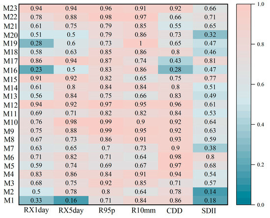
Figure 21.
The values of S in extreme precipitation indices for 23 CMIP6 GCMs from 1961 to 2010.
4. Discussion
The GCMs overestimate TNn and underestimate TXx in this study, and these findings are very much in agreement with the study carried out by Alexander et al. [37] in Australia. For the extreme precipitation indices, GCMs underestimated RX1day, RX5day, CDD and SDII, and similar situations occurred in the United States [38] and Thailand [39]. However, our study found that R10mm was overestimated, which is different from the results of Lei et al. [40]. The complexity of the climate system and the representation of the physical processes carried out by GCMs can lead to difficulties for models in accurately simulating extreme climate events [18]. Different parameterization schemes can affect the results [41,42]. For instance, TXx is directly influenced by solar radiation, whereas TNn is influenced by atmospheric radiative cooling and surface heat release, and these processes may be treated using different parameterization schemes in GCMs. Due to the low resolution of GCMs, GCMs may not be able to capture small-scale temperature changes, especially in regions with complex topography [43]. Previous studies [8,17] have demonstrated that increasing the spatial resolution of GCMs can improve the simulation of extreme climate events to some extent. However, high-spatial-resolution GCMs may increase simulation uncertainty due to their intrinsic complexity, which includes more parameters and processes [9]. Differences in observations, study periods, and downscaling methods, etc., may also lead to different biases.
The performance of GCMs can also vary in regions with different topographic complexity, as noted by Zhu et al. [3]. Our study shows spatial heterogeneity in the distribution of the biases. The higher biases are mainly located in the southern, eastern and northwestern regions of TNPC. This may be due to the proximity of the southeastern part of TNPC to the ocean, which affects the outputs of GCMs and causes higher biases [44]. In the northwestern region, higher latitudes may intensify temperature and precipitation variability, which may influence the simulation results [19]. TNPC is close to the Yellow Sea and Bohai Sea, with typical monsoon characteristics. Globally, the monsoon area is the region with the strongest extreme precipitation and the largest contribution to the total precipitation [45]. The influence of topography and monsoon on extreme climate events should be focused on when making future projections.
No single model can accurately reproduce the spatiotemporal variations of all indices. Most GCMs perform well in terms of spatiotemporal variations in FD and TNn, with the exception of M11 in simulating FD (as shown in Figure 22). However, GCMs perform poorly for TXx and DTR. It is worth noting that M15 performs well in simulating the spatiotemporal variation in all indices except DTR. Most GCMs effectively reproduce the temporal variations of RX1day, RX5day and CDD (Figure 23). About half of the GCMs show good results in the simulation of R95p, R10mm and SDII. As for M10, it performs well in the spatiotemporal simulation across all extreme precipitation indices. It is worth noting that the GCMs perform better in the spatiotemporal simulation of extreme temperature compared to the simulation of extreme precipitation, and this is consistent with the findings of Zhu et al. [41]. In contrast to extreme precipitation, extreme temperature is mainly influenced by relatively simple physical processes such as atmospheric pressure, solar radiation and greenhouse gas concentrations [46], and GCMs are usually able to accurately simulate atmospheric concentrations of greenhouse gases, which are a key factor influencing temperature [47]. However, precipitation processes involve more complex physical processes [48,49], such as evaporation, condensation and precipitation of water vapor, and cloud formation and evolution, which can be more complex and uncertain in spatial and temporal simulations [7,50], making it more difficult to accurately simulate extreme precipitation events.
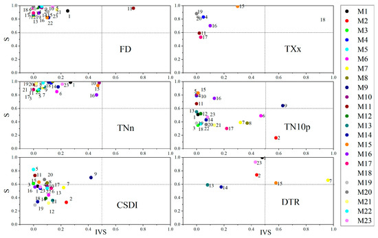
Figure 22.
Scatterplot of extreme temperature indices for 23 GCMs based on IVS (horizontal axis) and S (vertical axis). GCMs situated in the upper left quadrant demonstrate better spatiotemporal simulation performance, while those in the lower right quadrant exhibit the poorest simulation performance.
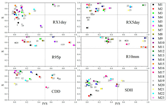
Figure 23.
Scatterplot of extreme precipitation indices for 23 GCMs based on IVS and S.
Furthermore, previous studies have shown that GCMs themselves have significant systematic biases, and bias revision techniques can effectively reduce the bias between model projections and actual observations. Yang et al. [51] found that the quality of bias-corrected data was superior to that of individual CMIP6 models with respect to extreme events. Additionally, downscaling techniques are considered a key method to improve the performance of meteorological models [52]. The study carried out by Wei et al. [43] pointed out that increasing the horizontal resolution of the model can improve the ability of GCMs to simulate average and extreme precipitation to some extent. Given the complexity of the climate system, a single climate model may not be able to capture all meteorological variations, and multi-model ensembles can improve the accuracy and reliability of projections by integrating the predictions of multiple models [18,51,53]. Since each model has its own uncertainties and limitations, combining projections from multiple models can effectively reduce these uncertainties and limitations. Taken together, how to accurately model extreme climate is a key issue for future research, and bias revision, downscaling, and model ensembles are key methods for achieving this goal. These methods not only improve the reliability of climate models, but also provide important support for more accurate simulations of climate change.
5. Conclusions
This study evaluated extreme climate indices over TPNC based on 23 CMIP6 GCMs outputs. The results of the study are as follows:
- (1)
- The GCMs could generally reproduce the spatial distribution of the extreme temperature indices, but underestimate most indices, with the exception of TNn, which shows a positive bias in 55.7% of the regional grids. TN10p and DTR exhibit negative biases in over 95% of the regional grids. The GCMs may perform better for spatial simulations of TXx and CSDI, with regional spatial biases of 1.17 °C and 1.91 d, respectively, while performing poorly in the spatial simulation of FD, with a regional spatial bias of 9d. Regionally, the spatial biases of the GCMs are larger in the northern and central parts of Heilongjiang Province and in most parts of Jilin and Liaoning Provinces.
- (2)
- The GCMs perform better in the spatial simulation of RX5day and R10mm, with regional spatial biases of 10.66% and 3.24 d, respectively, while the GCMs perform worse in the spatial simulation of R95p, with a regional spatial bias of 29.10%. Over 90% of grid simulations show positive biases for R95p and R10mm, but negative biases for CDD and SDII. RX1day and RX5day also exhibit negative biases in over 80% and 54% of the regional grids, respectively. Regionally, the simulated extreme precipitation in northern and southeastern Heilongjiang Province and northeastern Jilin Province shows positive biases.
- (3)
- The GCMs reproduce the interannual variability of FD, TNn, TN10p and CSDI (IVS < 0.5) but show inconsistency in capturing the interannual variabilities of TXx and DTR (IVS > 0.9). M15 has the best ability to reproduce interannual variability in six extreme temperature indices (IVS < 0.6). The GCMs perform well in temporal simulations of RX1day, RX5day, CDD and SDII (IVS < 0.65), but are poor in R95p and R10mm (IVS > 0.9). M1 and M10 reproduce the interannual variability well in six extreme precipitation indices (IVS < 0.4).
- (4)
- The GCMs have the strongest spatial simulation for FD and TNn (R > 0.85, σ ≈ 1, 0.25 < E′ < 0.75, S > 8). For TN10p and CSDI, the agreement between GCMs outputs and observations is generally poor (R < 0.20, σ ≈ 0.5, E′ > 1, S < 0.5). The spatial simulation of extreme temperature indices is best for M5, M9 and M15, while M2, M17, M18 and M19 perform poorly. The spatial simulation of the RX1day, RX5day, CDD and SDII (0.6 < R < 0.9, 0.4 < σ < 0.7, E’ < 1.0) is generally good in most GCMs. Except M1, M16 and M19, the other GCMs perform well in the spatial simulation of the R95p and R10mm.
Author Contributions
Methodology, H.X. and X.Z.; validation, K.P., Z.A. and X.Z.; formal analysis, Y.Z.; investigation, K.P. and H.S.; resources, Z.A. and H.S.; data curation, H.S.; writing—original draft preparation, H.X. and Y.Z.; writing—review and editing, H.X., Y.Z. and K.P. All authors have read and agreed to the published version of the manuscript.
Funding
This research was funded by the Key Scientific and Technological Project of Henan Province, China, grant number 222102320286; National Natural Science Foundation of China, grant number 51979106; and Henan Science and Technology R&D Program Joint Fund Project, grant number 232103810102.
Data Availability Statement
The datasets used and/or analyzed during the current study are available from the corresponding author on reasonable request.
Conflicts of Interest
The authors declare no conflict of interest.
References
- IPCC Climate Change 2021: The Physical Science Basis. Contribution of Working Group I to the Sixth Assessment Report of the Intergovernmental Panel on Climate Change; Cambridge University Press: Cambridge, UK; Available online: https://www.ipcc.ch/report/ar6/wg1/ (accessed on 1 June 2023).
- Sun, P.; Zou, Y.; Yao, R.; Ma, Z.; Bian, Y.; Ge, C.; Lv, Y. Compound and successive events of extreme precipitation and extreme runoff under heatwaves based on CMIP6 models. Sci. Total Environ. 2023, 878, 162980. [Google Scholar] [CrossRef] [PubMed]
- Liu, Z.; Huang, J.; Xiao, X.; Tong, X. The capability of CMIP6 models on seasonal precipitation extremes over Central Asia. Atmos. Res. 2022, 278, 106364. [Google Scholar] [CrossRef]
- World Meteorological Organization. State of Climate in 2021: Extreme Events and Major Impacts. 2021. Available online: https://public.wmo.int/en/media/press-release/state-of-climate-2021-extreme-events-and-major-impacts (accessed on 9 June 2023).
- Intergovernmental Panel on Climate Change, IPCC (Ed.) Global Warming of 15 °C: IPCC Special Report on Impacts of Global Warming of 1.5 °C above Pre-Industrial Levels in Context of Strengthening Response to Climate Change, Sustainable Development, and Efforts to Eradicate Roverty; Cambridge University Press: Cambridge, UK, 2018; pp. 601–616. [Google Scholar]
- Li, H.; Chen, H.; Wang, H.; Yu, E. Future precipitation changes over China under 1.5 °C and 2.0 °C global warming targets by using CORDEX regional climate models. Sci. Total Environ. 2018, 640–641, 543–554. [Google Scholar] [CrossRef] [PubMed]
- Qin, P.; Xie, Z.; Zou, J.; Liu, S.; Chen, S. Future Precipitation Extremes in China under Climate Change and Their Physical Quantification Based on a Regional Climate Model and CMIP5 Model Simulations. Adv. Atmos. Sci. 2021, 38, 460–479. [Google Scholar] [CrossRef]
- Fan, X.; Miao, C.; Duan, Q.; Shen, C.; Wu, Y. The performance of CMIP6 versus CMIP5 in simulating temperature extremes over the global land surface. J. Geophys. Res. Atmos. 2020, 125, e2020JD033031. [Google Scholar] [CrossRef]
- Liang, J.; Meng, C.; Wang, J.; Pan, X.; Pan, Z. Projections of mean and extreme precipitation over China and their resolution dependence in the HighResMIP experiments. Atmos. Res. 2023, 293, 106932. [Google Scholar] [CrossRef]
- Eyring, V.; Bony, S.; Meehl, G.A.; Senior, C.A.; Stevens, B.; Stouffer, R.J.; Taylor, K.E. Overview of the Coupled Model Intercomparison Project Phase 6 (CMIP6) experimental design and organization. Geosci. Model Dev. 2016, 9, 1937–1958. [Google Scholar] [CrossRef]
- Meehl, G.; Boer, G.; Covey, C.; Latif, M.; Ronald, S. CMIP Coupled Model Intercomparison Project. Bull. Am. Meteorol. Soc. 2000, 81, 313–318. [Google Scholar] [CrossRef]
- Raju, K.S.; Kumar, D.N. Review of approaches for selection and ensembling of GCMs. J. Water Clim. Chang. 2020, 11, 577–599. [Google Scholar] [CrossRef]
- Touzé-Peiffer, L.; Barberousse, A.; Le Treut, H. The Coupled Model Intercomparison Project: History, Uses, and Structural Effects on Climate Research. WIREs Clim. Chang. 2020, 11, e648. [Google Scholar] [CrossRef]
- Grose, M.R.; Narsey, S.; Delage, F.P.; Dowdy, A.J.; Bador, M.; Boschat, G.; Chung, C.; Kajtar, J.B.; Rauniyar, S.; Freund, M.B.; et al. Insights from CMIP6 for Australia’s Future Climate. Earths Future 2020, 8, e2019EF001469. [Google Scholar] [CrossRef]
- Zamani, Y.; Hashemi Monfared, S.A.; Azhdari Moghaddam, M.; Hamidianpour, M. A comparison of CMIP6 and CMIP5 projections for precipitation to observational data: The case of Northeastern Iran. Theor. Appl. Climatol. 2020, 142, 1613–1623. [Google Scholar] [CrossRef]
- Wyser, K.; van Noije, T.; Yang, S.; von Hardenberg, J.; O’Donnell, D.; Döscher, R. On the increased climate sensitivity in the EC-Earth model from CMIP5 to CMIP6. Geosci. Model Dev. 2020, 13, 3465–3474. [Google Scholar] [CrossRef]
- Chen, H.; Sun, J.; Lin, W.; Xu, H. Comparison of CMIP6 and CMIP5 models in simulating climate extremes. Sci. Bull. 2020, 65, 1415–1418. [Google Scholar] [CrossRef] [PubMed]
- Cui, T.; Li, C.; Tian, F. Evaluation of temperature and precipitation simulations in CMIP6 models over the Tibetan Plateau. Earth Space Sci. 2021, 8, e2020EA001620. [Google Scholar] [CrossRef]
- Mequanint, F.; Streck, T.; Tesfaye, K.; Gayler, S.; Weber, T. Comprehensive assessment of climate extremes in high-resolution CMIP6 projections for Ethiopia. Front. Environ. Sci. 2023, 11, 1127265. [Google Scholar]
- Ha, T.T.V.; Fan, H.; Shuang, L. Climate change impact assessment on Northeast China’s grain production. Environ. Sci. Pollut. Res. 2021, 28, 14508–14520. [Google Scholar] [CrossRef]
- Yu, X.; Ma, Y. Spatial and temporal analysis of extreme climate events over Northeast China. Atmosphere 2022, 13, 1197. [Google Scholar] [CrossRef]
- Liu, S.; Zhou, Z.; Liu, J.; Li, J.; Wang, P.; Li, C.; Xie, X.; Jia, Y.; Wang, H. Analysis of the runoff component variation mechanisms in the cold region of Northeastern China under climate change. Water 2022, 14, 3170. [Google Scholar] [CrossRef]
- Wei, J.; Liu, X.; Zhou, B. Sensitivity of vegetation to climate in mid-to-high latitudes of Asia and future vegetation projections. Remote Sens. 2023, 15, 2648. [Google Scholar] [CrossRef]
- He, X.; Jiang, C.; Wang, J.; Wang, X. Comparison of CMIP6 and CMIP5 models performance in simulating temperature in Northeast China. Chin. J. Geophys. 2022, 65, 4194–4207. (In Chinese) [Google Scholar]
- Xu, T.; Pang, H.; Zhan, Z.; Guo, H.; Wu, S.; Zhang, W.; Hou, S. Characteristics of water vapor isotopes and moisture sources for short-duration heavy rainfall events in Nanjing, eastern China. J. Hydrol. 2023, 622, 129731. [Google Scholar] [CrossRef]
- Guan, J.; Yao, J.; Li, M.; Li, D.; Zheng, J. Historical changes and projected trends of extreme climate events in Xinjiang, China. Clim. Dyn. 2022, 59, 1753–1774. [Google Scholar] [CrossRef]
- Chen, Y.D.; Li, J.; Zhang, Q.; Gu, X. Projected changes in seasonal temperature extremes across China from 2017 to 2100 based on statistical downscaling. Glob. Planet Chang. 2018, 166, 30–40. [Google Scholar] [CrossRef]
- Chen, F.; Liu, C. Estimation of the spatial rainfall distribution using inverse distance weighting (IDW) in the middle of Taiwan. Paddy Water Environ. 2012, 10, 209–222. [Google Scholar] [CrossRef]
- Mastyło, M. Bilinear interpolation theorems and applications. J. Funct. Anal. 2013, 265, 185–207. [Google Scholar] [CrossRef]
- PL, F.; Alexander, L.; Della-Marta, P.; Gleason, B.; Haylock, M.; Klein, T.; TC, P. Observed coherent changes in climatic extremes during 2nd half of the 20th century. Clim. Res. 2002, 19, 193–212. [Google Scholar]
- Zhang, X.; Alexander, L.; Hegerl, G.C.; Jones, P.; Tank, A.K.; Peterson, T.C.; Trewin, B.; Zwiers, F.W. Indices for monitoring changes in extremes based on daily temperature and precipitation data. WIREs Clim. Chang. 2011, 2, 851–870. [Google Scholar] [CrossRef]
- Zhu, C.; Yue, Q.; Huang, J. Projections of mean and extreme precipitation using the CMIP6 Model: A study of the Yangtze River Basin in China. Water 2023, 15, 3043. [Google Scholar] [CrossRef]
- Ávila, Á.; Guerrero, F.C.; Escobar, Y.C.; Justino, F. Recent precipitation trends and floods in the Colombian Andes. Water 2019, 11, 379. [Google Scholar] [CrossRef]
- Chen, W.; Jiang, Z.; Li, L. Probabilistic projections of climate change over China under the SRES A1B scenario using 28 AOGCMs. J. Clim. 2011, 24, 4741–4756. [Google Scholar] [CrossRef]
- Taylor, K. Summarizing multiple aspects of model performance in a single diagram. J. Geophys. Res. 2001, 106, 7183–7192. [Google Scholar] [CrossRef]
- Ullah, W.; Wang, G.; Lou, D.; Ullah, S.; Bhatti, A.S.; Ullah, S.; Karim, A.; Hagan, D.F.T.; Ali, G. Large-scale atmospheric circulation patterns associated with extreme monsoon precipitation in Pakistan during 1981–2018. Atmos. Res. 2021, 253, 105489. [Google Scholar] [CrossRef]
- Alexander, L.V.; Arblaster, J.M. Historical and projected trends in temperature and precipitation extremes in Australia in observations and CMIP5. Weather Clim. Extrem. 2017, 15, 34–56. [Google Scholar] [CrossRef]
- Schoof, J.T.; Robeson, S.M. Projecting changes in regional temperature and precipitation extremes in the United States. Weather Clim. Extrem. 2016, 11, 28–40. [Google Scholar] [CrossRef]
- Rojpratak, S.; Supharatid, S. Regional extreme precipitation index: Evaluations and projections from the multi-model ensemble CMIP5 over Thailand. Weather Clim. Extrem. 2022, 37, 100475. [Google Scholar] [CrossRef]
- Lei, X.; Xu, C.; Liu, F.; Song, L.; Cao, L.; Suo, N. Evaluation of CMIP6 Models and Multi-Model Ensemble for Extreme Precipitation over Arid Central Asia. Remote Sens. 2023, 15, 2376. [Google Scholar] [CrossRef]
- Zhu, H.; Jiang, Z.; Li, J.; Li, W.; Sun, C.; Li, L. Does CMIP6 inspire more confidence in simulating climate extremes over China? Adv. Atmos. Sci. 2020, 37, 1119–1132. [Google Scholar] [CrossRef]
- Hu, G.; Franzke, C.L.E. Evaluation of daily precipitation extremes in reanalysis and gridded observation-based data sets over Germany. Geophys. Res. Lett. 2020, 47, e2020GL089624. [Google Scholar] [CrossRef]
- Wei, L.; Xin, X.; Li, Q.; Wu, Y.; Tang, H.; Li, Y.; Yang, B. Simulation and projection of climate extremes in China by multiple Coupled Model Intercomparison Project Phase 6 models. Int. J. Climatol. 2023, 43, 219–239. [Google Scholar] [CrossRef]
- Dirmeyer, P.A. Land-sea geometry and its effect on monsoon circulations. J. Geophys. Res. Atmos. 1998, 103, 11555–11572. [Google Scholar] [CrossRef]
- Zhang, W.; Zhou, T. Significant increases in extreme precipitation and the associations with global warming over the global land monsoon regions. J. Clim. 2019, 32, 8465–8488. [Google Scholar] [CrossRef]
- Kong, X.; Wang, A.; Bi, X.; Wang, D. Assessment of temperature extremes in China using RegCM4 and WRF. Adv. Atmos. Sci. 2019, 36, 363–377. [Google Scholar] [CrossRef]
- Landwehrs, J.; Feulner, G.; Petri, S.; Sames, B.; Wagreich, M. Investigating mesozoic climate trends and sensitivities with a large ensemble of climate model simulations. Paleoceanogr. Paleoclimatol. 2021, 36, e2020PA004134. [Google Scholar] [CrossRef]
- Zhang, F.; Huang, T.; Man, W.; Hu, H.; Long, Y.; Li, Z.; Pang, Z. Contribution of recycled moisture to precipitation: A modified D-Excess-Based Model. Geophys. Res. Lett. 2021, 48, e2021GL095909. [Google Scholar] [CrossRef]
- Zhang, W.; Furtado, K.; Wu, P.; Zhou, T.; Chadwick, R.; Marzin, C.; Rostron, J.; Sexton, D. Increasing precipitation varia-bility on daily-to-multiyear time scales in a warmer world. Sci. Adv. 2021, 7, f8021. [Google Scholar] [CrossRef]
- John, A.; Douville, H.; Ribes, A.; Yiou, P. Quantifying CMIP6 model uncertainties in extreme precipitation projections. Weather Clim. Extrem. 2022, 36, 100435. [Google Scholar] [CrossRef]
- Yang, Y.; Zhang, Y.; Gao, Z.; Pan, Z.; Zhang, X. Historical and projected changes in temperature extremes over China and the inconsistency between multimodel ensembles and individual models from CMIP5 and CMIP6. Earth Space Sci. 2023, 10, e2022EA002514. [Google Scholar] [CrossRef]
- Xu, Z.; Han, Y.; Tam, C.; Yang, Z.; Fu, C. Bias-corrected CMIP6 global dataset for dynamical downscaling of the historical and future climate (1979–2100). Sci. Data 2021, 8, 293. [Google Scholar] [CrossRef]
- Ma, Z.; Sun, P.; Zhang, Q.; Zou, Y.; Lv, Y.; Li, H.; Chen, D. The characteristics and evaluation of future droughts across China through the CMIP6 multi-model ensemble. Remote Sens. 2022, 14, 1097. [Google Scholar] [CrossRef]
Disclaimer/Publisher’s Note: The statements, opinions and data contained in all publications are solely those of the individual author(s) and contributor(s) and not of MDPI and/or the editor(s). MDPI and/or the editor(s) disclaim responsibility for any injury to people or property resulting from any ideas, methods, instructions or products referred to in the content. |
© 2023 by the authors. Licensee MDPI, Basel, Switzerland. This article is an open access article distributed under the terms and conditions of the Creative Commons Attribution (CC BY) license (https://creativecommons.org/licenses/by/4.0/).