
A Horizontal Distribution Model of Static Ice Cover Generated by Static and Dynamic Water Considering the Heat Transfer of Riverbanks


Abstract
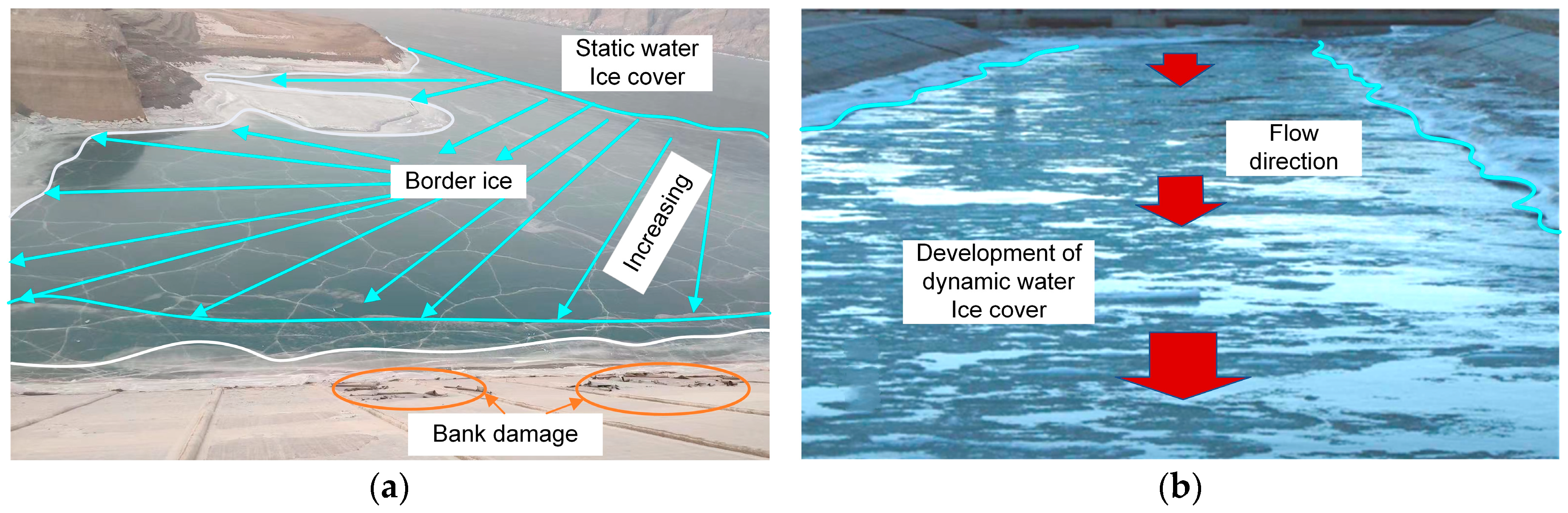
:1. Introduction
2. Horizontal Distribution Model of Static Ice Cover Considering Heat Transfer of River Banks
2.1. Temperature Control Equation
2.1.1. Water Flow Temperature Calculation Model
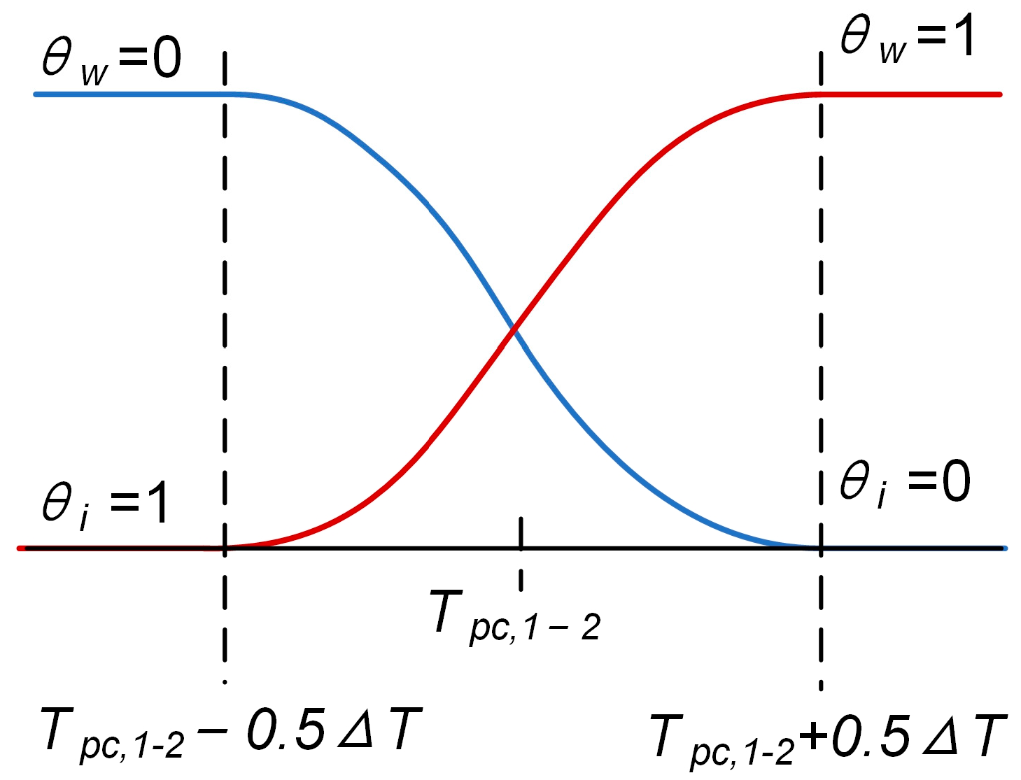
2.1.2. Water Flow Icing Model
2.1.3. Coupled Moisture-Heat Transport Model of Frozen Soil on Banks
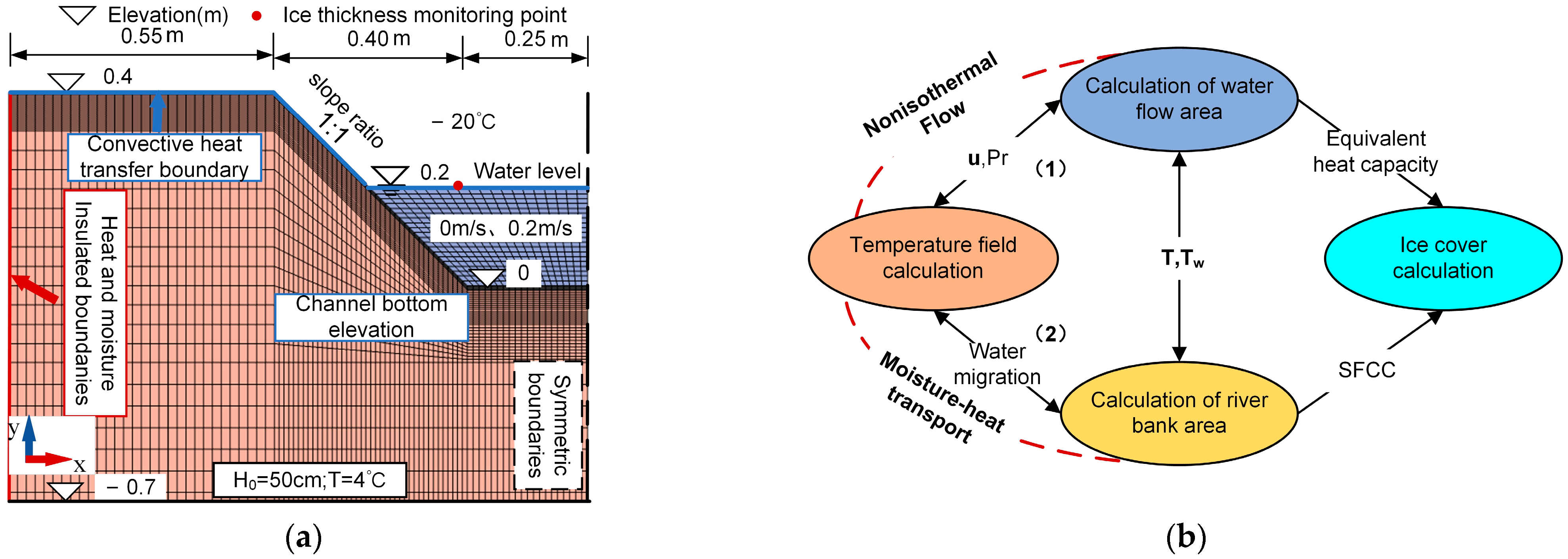
2.2. Model Boundary Condition and Solving Process
3. Results
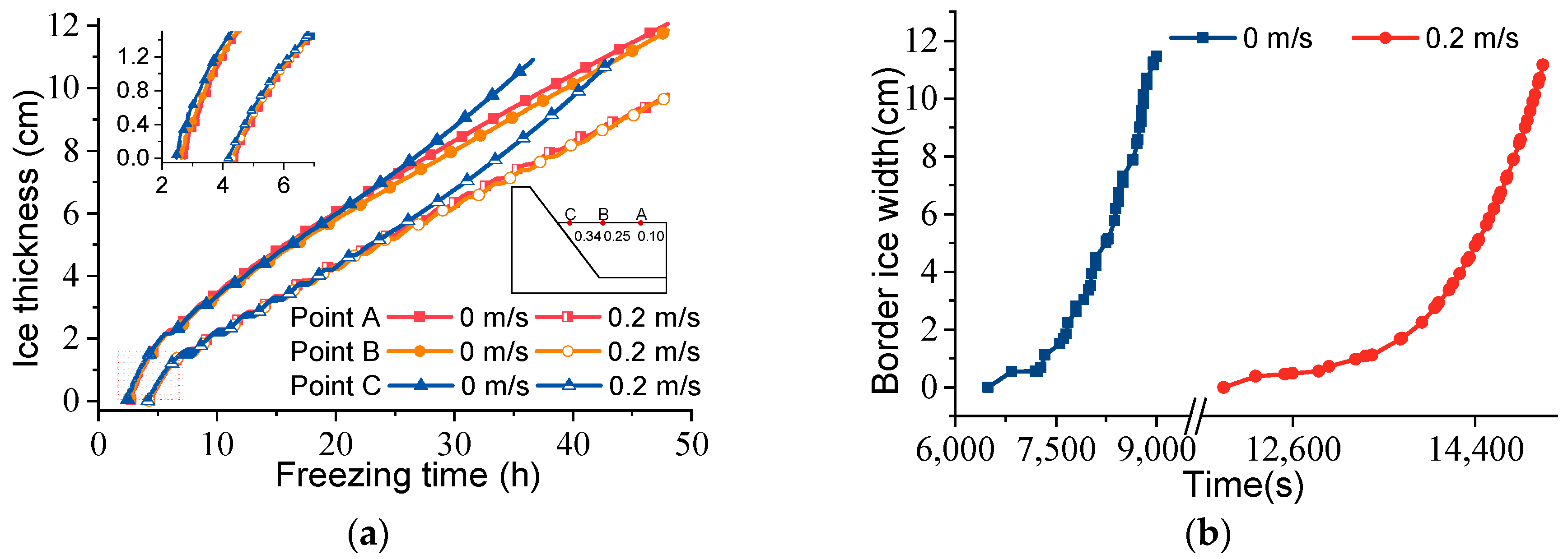
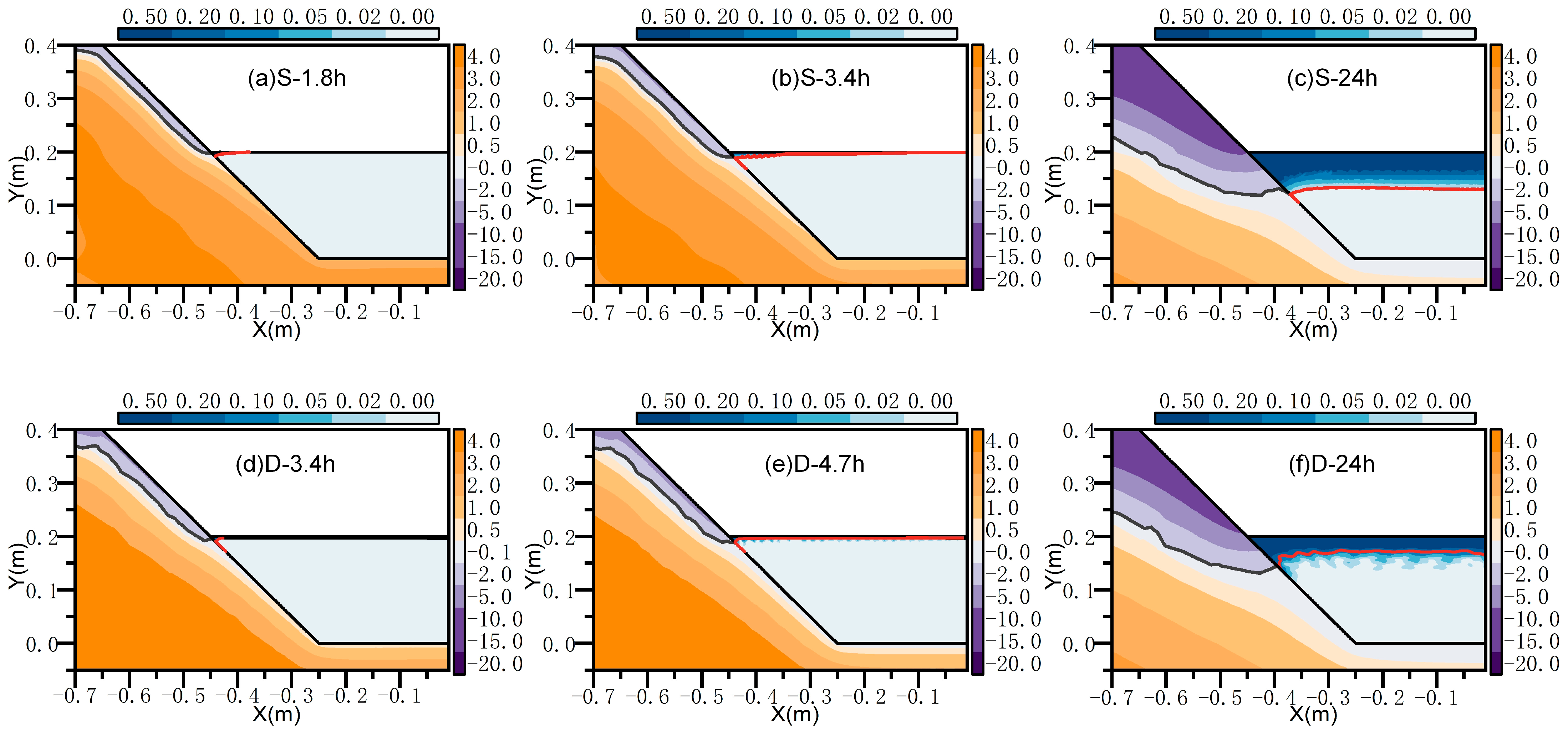
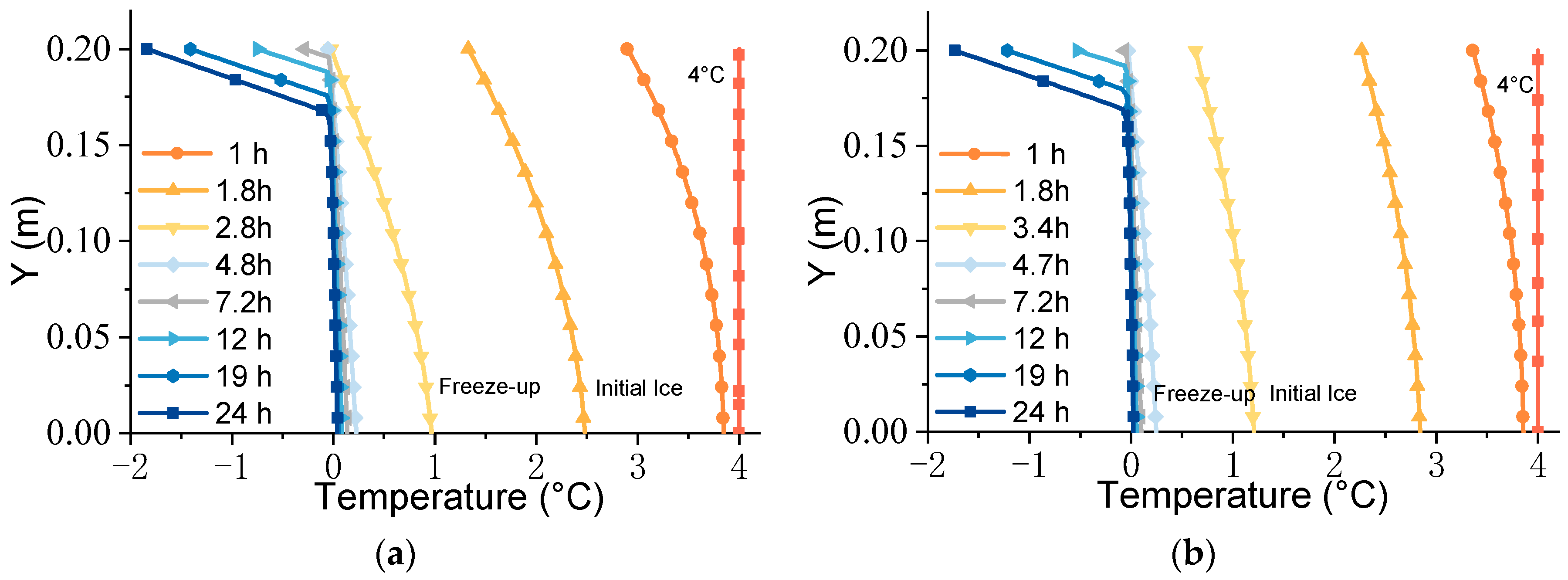
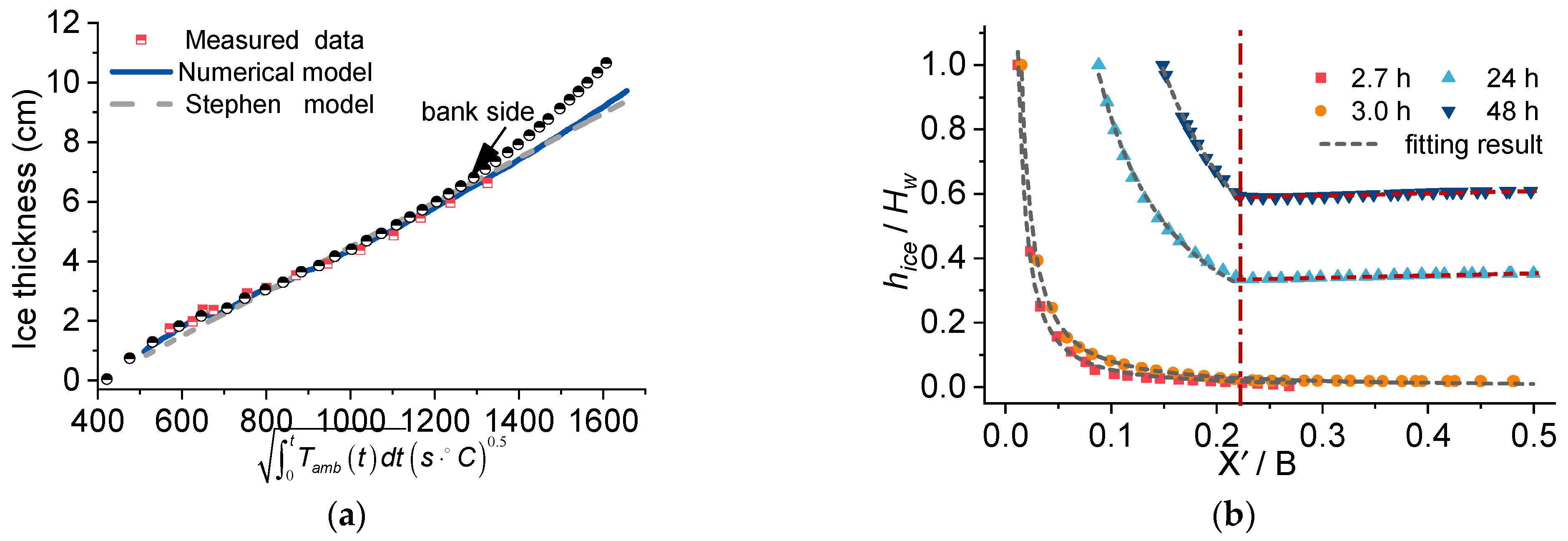
3.1. Analysis of Ice Thickness Growth Generated by Static and Dynamic Water
3.2. Coupling Analysis of Ice Thickness Growth and Riverbank Freezing Process
4. Discussion
4.1. The Influence of Temperature and Water Velocity on the Formation of Static Ice Cover
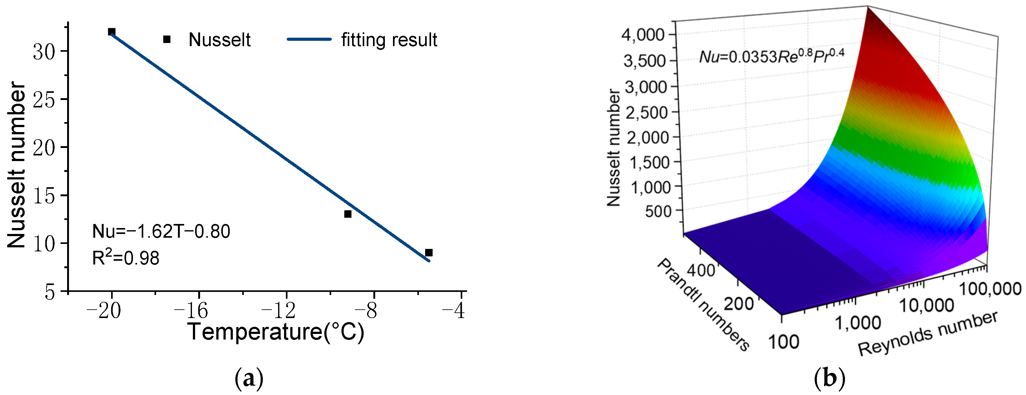
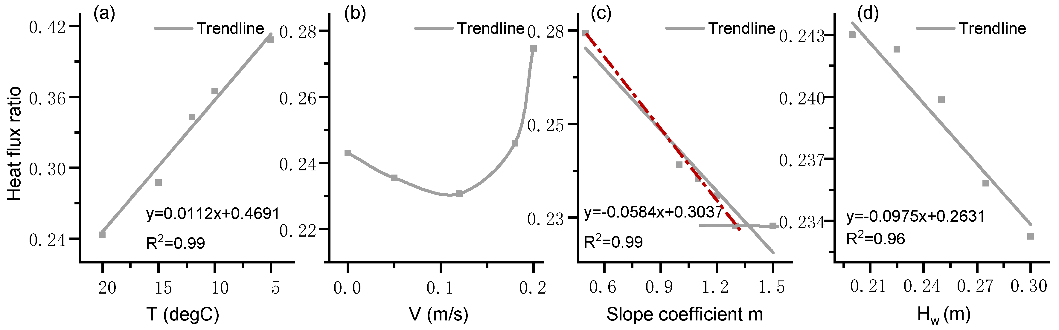
4.1.1. Analysis of Model Coupling Parameters
4.1.2. Analysis of the Horizontal Difference of Static Ice Cover
4.1.3. The Influence of Riverbed Heat Transfer on Water and Heat Exchange
4.2. Horizontal Distribution Regression Model of Ice Cover
5. Conclusions
Author Contributions
Funding
Data Availability Statement
Acknowledgments
Conflicts of Interest
References
- Saadé, R.G.; Sarraf, S. Simulation of Ice Cover Melting in Turbulent Flow. Int. J. Numer. Methods Heat Fluid Flow 1995, 5, 647–663. [Google Scholar] [CrossRef]
- Rokaya, P.; Budhathoki, S.; Lindenschmidt, K.-E. Trends in the Timing and Magnitude of Ice-Jam Floods in Canada. Sci. Rep. 2018, 8, 5834. [Google Scholar] [CrossRef]
- Adalaiti, H.J.; Yu, S.S. Study and Prospect of Ice Damage Prevention and Control in Xinjiang’s Water Conveyance Projects. J. Water Resour. Archit. Eng. 2010, 8, 46–49. (In Chinese) [Google Scholar]
- Yang, K. Advances of ice hydraulics, ice regime observation and forecasting in rivers. J. Hydraul. Eng. 2018, 49, 81–91. (In Chinese) [Google Scholar] [CrossRef]
- Guo, X.; Wang, T.; Fu, H.; Pan, J.; Lu, J.; Guo, Y.; Li, J. Progress and Trend in the Study of River Ice Hydraulics. Theor. Appl. Mech. 2021, 53, 655–671. (In Chinese) [Google Scholar]
- Shen, H.T. River Ice Processes. In Advances in Water Resources Management; Wang, L.K., Yang, C.T., Wang, M.-H.S., Eds.; Springer International Publishing: Cham, Switzerland, 2016; pp. 483–530. ISBN 978-3-319-22923-2. [Google Scholar]
- Peters, M.; Dow, K.; Clark, S.P.; Malenchak, J.; Danielson, D. Experimental Investigation of the Flow Characteristics beneath Partial Ice Covers. Cold Reg. Sci. Technol. 2017, 142, 69–78. [Google Scholar] [CrossRef]
- Pan, J.; Shen, H.T. Modeling Ice Cover Effect on River Channel Bank Stability. Environ. Fluid Mech. 2022, 22, 1121–1133. [Google Scholar] [CrossRef]
- Duan, W.; Huang, G.; Yang, J.; Liu, M. Ice regime analysis and safe dispatch research on long distance water diversion project in winter. South-North Water Transf. Water Sci. Technol. 2016, 14, 96–104. (In Chinese) [Google Scholar] [CrossRef]
- Shen, H.T. Mathematical Modeling of River Ice Processes. Cold Reg. Sci. Technol. 2010, 62, 3–13. [Google Scholar] [CrossRef]
- Svensson, U.; Billfalk, L.; Hammar, L. A Mathematical Model of Border-Ice Formation in Rivers. Cold Reg. Sci. Technol. 1989, 16, 179–189. [Google Scholar] [CrossRef]
- Huang, F.; Shen, H.T.; Knack, I. Modeling Border Ice Formation and Cover Progression in Rivers. In Proceedings of the IAHR International Symposium on Ice, Dalian, China, 11–15 June 2012. [Google Scholar]
- Mao, Z.; Dong, Z.; Chen, C. Review on mathematical simulation of river ice. Water Power 1996, 12, 58–61. (In Chinese) [Google Scholar]
- Mao, Z.; Chen, C. Simulation of Heat Transfer between Streambed and River Flow. Water Resour. Hydropower Eng. 1999, 5, 11–13. (In Chinese) [Google Scholar] [CrossRef]
- Bernard, M. Comparison of Field Data with Theories on Ice Cover Progression in Large Rivers. Can. J. Civ. Eng. 2011, 11, 798–814. [Google Scholar] [CrossRef]
- Shen, H.T.; Yapa, P.D. A Unified Degree-Day Method for River Ice Cover Thickness Simulation. Can. J. Civ. Eng. 1985, 12, 54–62. [Google Scholar] [CrossRef]
- Yang, K.; Guo, X.; Wang, T.; Fu, H.; Pan, J. Effects of solar radiation and ground temperature on water temperature under ice cover. J. Hydraul. Eng. 2022, 53, 530–538+548. (In Chinese) [Google Scholar] [CrossRef]
- Lian, J.; Zhao, X. Radiation degree-day method for predicting the development of ice cover thickness under the hydrostatic and non-hydrostatic conditions. J. Hydraul. Eng. 2011, 42, 1261–1267. (In Chinese) [Google Scholar] [CrossRef]
- Gordon, M. Greene Simulation of Ice-Cover Growth and Decay in One Dimension on the Upper St. Lawrence River. Available online: https://repository.library.noaa.gov/view/noaa/10432 (accessed on 30 June 2023).
- Khan, Z.H.; Ahmad, R.; Sun, L. Effect of Instantaneous Change of Surface Temperature and Density on an Unsteady Liquid–Vapour Front in a Porous Medium. Exp. Comput. Multiph. Flow 2020, 2, 115–121. [Google Scholar] [CrossRef]
- Peters, G.W.M.; Baaijens, F.P.T. Modelling of Non-Isothermal Viscoelastic Flows. J. Non-Newton. Fluid Mech. 1997, 68, 205–224. [Google Scholar] [CrossRef]
- Xiao, H.; Dong, Z.; Long, R.; Yang, K.; Yuan, F. A Study on the Mechanism of Convective Heat Transfer Enhancement Based on Heat Convection Velocity Analysis. Energies 2019, 12, 4175. [Google Scholar] [CrossRef]
- Lienhard, J.H. A Heat Transfer Textbook; Phlogiston Press: Cambridge, MA, USA, 2011; Available online: https://ahtt.mit.edu (accessed on 3 August 2023).
- Kays, W.M. Turbulent Prandtl Number—Where Are We? Asme Trans. J. Heat Transf. 1994, 116, 284–295. [Google Scholar] [CrossRef]
- Thonon, M.; Fraisse, G.; Zalewski, L.; Pailha, M. Towards a Better Analytical Modelling of the Thermodynamic Behaviour of Phase Change Materials. J. Energy Storage 2020, 32, 101826. [Google Scholar] [CrossRef]
- Moench, S.; Dittrich, R. Influence of Natural Convection and Volume Change on Numerical Simulation of Phase Change Materials for Latent Heat Storage. Energies 2022, 15, 2746. [Google Scholar] [CrossRef]
- Jiang, H.; Liu, Q.; Wang, Z.; Gong, J.; Li, L. Frost Heave Modelling of the Sunny-Shady Slope Effect with Moisture-Heat-Mechanical Coupling Considering Solar Radiation. Sol. Energy 2022, 233, 292–308. [Google Scholar] [CrossRef]
- Liu, Q.; Wang, Z.; Li, Z.; Wang, Y. Transversely Isotropic Frost Heave Modeling with Heat–Moisture–Deformation Coupling. Acta Geotech. 2020, 15, 1273–1287. [Google Scholar] [CrossRef]
- Harlan, R.L. Analysis of Coupled Heat-Fluid Transport in Partially Frozen Soil. Water Resour. Res. 1973, 9, 1314–1323. [Google Scholar] [CrossRef]
- Hansson, K.; Imnek, J.; Mizoguchi, M.; Lundin, L.C.; Van Genuchten, M.T. Water Flow and Heat Transport in Frozen Soil: Numerical Solution and Freeze–Thaw Applications. Vadose Zone J. 2004, 3, 693–704. [Google Scholar] [CrossRef]
- Liu, X.; Liu, J.; Tian, Y.; Shen, Y.; Liu, J. A Frost Heaving Mitigation Method with the Rubber-Asphalt-Fiber Mixture Cylinder. Cold Reg. Sci. Technol. 2020, 169, 102912. [Google Scholar] [CrossRef]
- Li, S.; Zhang, M.; Tian, Y.; Pei, W.; Zhong, H. Experimental and Numerical Investigations on Frost Damage Mechanism of a Canal in Cold Regions. Cold Reg. Sci. Technol. 2015, 116, 1–11. [Google Scholar] [CrossRef]
- Xu, X. Physics of Frozen Soil; Physics of Frozen Soil: Beijing, China, 2010; ISBN 978-7-03-028867-7. [Google Scholar]
- Lu, N.; Likos, W.J. Unsaturated Soil Mechanics; John Wiley & Sons, Inc.: Hoboken, NJ, USA, 2004; Available online: https://webapps.unitn.it/Biblioteca/it/Web/EngibankFile/5802626.pdf (accessed on 15 June 2023).
- Nan, L.I.; Tuo, Y.C.; Deng, Y.; Jia, L.I.; Liang, R.F.; Rui-Dong, A.N. Heat Transfer at Ice-Water Interface under Conditions of Low Flow Velocities. J. Hydrodyn. 2016, 28, 603–609. [Google Scholar] [CrossRef]
- Sarraf, S.; Zhang, X.T. Modeling Ice-Cover Melting Using a Variable Heat Transfer Coefficient. J. Eng. Mech. 1996, 122, 930–938. [Google Scholar] [CrossRef]
- Dong, S.; Cui, H. Analysis of Calculating Formula and Improvement of Empirical Formula for Saturation Vapour Pressure. Q. J. Appl. Meteorol. 1992, 3, 501–508. (In Chinese) [Google Scholar]
- Yang, K. Heat exchange model between river-lake and atmosphere during ice age. J. Hydraul. Eng. 2021, 52, 556–564+577. (In Chinese) [Google Scholar] [CrossRef]
- Hanley, T.O.; Michel, B. Laboratory Formation of Border Ice and Frazil Slush. Can. J. Civ. Eng. 1977, 4, 153–160. [Google Scholar] [CrossRef]
- Michel, B.; Ramseier, R.O. Classification of River and Lake Ice. Can. Geotech. J. 1971, 8, 36–45. [Google Scholar] [CrossRef]
- Turcotte, B.; Morse, B. A Global River Ice Classification Model. J. Hydrol. 2013, 507, 134–148. [Google Scholar] [CrossRef]
- Blokhina, N.S.; Ordanovich, A.E. The Influence of Ice Cover on a Reservoir on the Development of a Spring Thermal Bar. Mosc. Univ. Phys. 2012, 67, 109–115. [Google Scholar] [CrossRef]
- Marsh, P.; Prowse, T.D. Water Temperature and Heat Flux at the Base of River Ice Covers. Cold Reg. Sci. Technol. 1987, 14, 33–50. [Google Scholar] [CrossRef]
- Yu, S.; Li, Q.; Song, L. Forecast of Ice State in Open Canal with Water Delivered in Ice Periods. China Rural Water Hydropower 2008, 9, 108–109+113. (In Chinese) [Google Scholar]


| Variable | Value | Variable | Value |
|---|---|---|---|
| ΔT (K) | 0.1 | λsa (W/(m·K)) | 0.024 |
| ρsp (kg/m3) | 2700 | L (kJ/kg) | 334 |
| ρsw (kg/m3) | 1000 | θs (1) | 0.43 |
| ρsi (kg/m3) | 931 | θr (1) | 0.03 |
| Csp (kJ/(m3·K)) | 2000 | α (1/m) | 0.38 |
| Csw (kJ/(m3·K)) | 4220 | m (1) | 0.36 |
| Csi (kJ/(m3·K)) | 1935 | Ks (m/s) | 2 × 10⁻⁷ |
| λsp (W/(m·K)) | 1.5 | a (1) | 6.89 |
| λsw (W/(m·K)) | 0.55 | b (1) | 0.57 |
| λsi (W/(m·K)) | 2.22 | ρd (kg/m3) | 0.7 |
| Case | T /°C | V /(m·s−1) | Hw /m | Slope Coefficient m | Initial Nu | Initial Ice Time /h | Freeze-Up Period /h | Ice Cover Thickness /cm | Thickness Difference /cm |
|---|---|---|---|---|---|---|---|---|---|
| 1 | −5 | 0.00 | 0.2 | 1.0 | 20 | 3.5 | 6.0 | 4.16 | 0.21 |
| 1 | −10 | 0.00 | 0.2 | 1.0 | 23 | 2.3 | 4.3 | 5.42 | 0.22 |
| 1 | −20 | 0.00 | 0.2 | 1.0 | 68 | 1.9 | 2.8 | 12.06 | 0.42 |
| 2 | −20 | 0.00 | 0.3 | 1.0 | 68 | 1.8 | 3.4 | 11.47 | 1.75 |
| 3 | −20 | 0.00 | 0.2 | 1.1 | 68 | 1.8 | 2.8 | 12.08 | 0.52 |
| 4 | −20 | 0.00 | 0.2 | 1.5 | 68 | 1.5 | 2.9 | 12.17 | 0.54 |
| 5 | −20 | 0.12 | 0.2 | 1.0 | 80 | 1.9 | 3.0 | 9.73 | 1.45 |
| 6 | −20 | 0.20 | 0.2 | 1.0 | 95 | 3.4 | 4.7 | 9.78 | 1.23 |
| Freezing Time (h) | a | c | R2 |
|---|---|---|---|
| 2.7 | 0.00221 | −1.3839 | 0.99632 |
| 3.0 | 0.00366 | −1.33003 | 0.99769 |
| 24 | 0.06690 | −1.08838 | 0.99426 |
| 48 | 0.12089 | −1.08153 | 0.99391 |
Disclaimer/Publisher’s Note: The statements, opinions and data contained in all publications are solely those of the individual author(s) and contributor(s) and not of MDPI and/or the editor(s). MDPI and/or the editor(s) disclaim responsibility for any injury to people or property resulting from any ideas, methods, instructions or products referred to in the content. |
© 2023 by the authors. Licensee MDPI, Basel, Switzerland. This article is an open access article distributed under the terms and conditions of the Creative Commons Attribution (CC BY) license (https://creativecommons.org/licenses/by/4.0/).
Share and Cite
Xue, B.; Wang, Z.; Liu, Q.; Li, H. A Horizontal Distribution Model of Static Ice Cover Generated by Static and Dynamic Water Considering the Heat Transfer of Riverbanks. Water 2023, 15, 3893. https://doi.org/10.3390/w15223893
Xue B, Wang Z, Liu Q, Li H. A Horizontal Distribution Model of Static Ice Cover Generated by Static and Dynamic Water Considering the Heat Transfer of Riverbanks. Water. 2023; 15(22):3893. https://doi.org/10.3390/w15223893
Chicago/Turabian StyleXue, Boxiang, Zhengzhong Wang, Quanhong Liu, and Hanxiang Li. 2023. "A Horizontal Distribution Model of Static Ice Cover Generated by Static and Dynamic Water Considering the Heat Transfer of Riverbanks" Water 15, no. 22: 3893. https://doi.org/10.3390/w15223893
APA StyleXue, B., Wang, Z., Liu, Q., & Li, H. (2023). A Horizontal Distribution Model of Static Ice Cover Generated by Static and Dynamic Water Considering the Heat Transfer of Riverbanks. Water, 15(22), 3893. https://doi.org/10.3390/w15223893