Abstract
Water demand forecasting plays an important role in the sustainable management of water resources, especially in countries facing water scarcity challenges, such as the United Arab Emirates (UAE). Al-Ain, the second-largest city within the Emirate of Abu Dhabi and the fourth largest in the UAE, faces the dual challenge of anticipated population growth and forthcoming development initiatives. These factors are set to exert added pressure on the city’s water resources. Hence, Al-Ain City requires an immediate assessment of future water demands as a critical step toward achieving sustainable development. The main objective of this study is to conduct a systematic analysis of historical consumption patterns and other relevant factors to predict future water demand and to present a water demand forecasting model to project the water requirements of Al-Ain City up to the year 2030. The proposed “Linear Forecast Model” for Al-Ain City is developed using the IWR-MAIN software (Version 6.0), with its core code developed by the U.S. Army Corps of Engineers’ Institute for Water Resources. The results of this model suggest that the total water demand is projected to increase by 45% by the year 2030. Among the sectors, the residential sector is expected to have the highest water demand, accounting for approximately 61% of the total water demand by 2030. The governmental and agricultural sectors are estimated to contribute 20% and 10% to the total demand, respectively, with the remaining 9% distributed across the other four sectors.
1. Introduction
Water demand forecasting is a crucial aspect of efficient water resource management and urban planning to achieve sustainable development. Accurate predictions of water demand are necessary since the lack of water resources has become a significant barrier to sustainable economic growth. Forecasting is a planning method that depends heavily on historical data to help future water supplies [1]. For several reasons, reliable water demand forecasting is necessary to make long-term operational and strategic decisions regarding the provision of public water [1]. Moreover, a water demand forecast serves as a cornerstone in water resources planning, enabling the preparation for projected future demands. Precise forecasts are instrumental in ensuring the provision of an adequate water supply, guaranteeing the delivery of safe and abundant water while minimizing associated costs [2]. Long-term water demand forecasting is imperative for proper water infrastructure and capital planning, as well as the formulation of effective water policies to prevent domestic water supply shortages and promote sustainable water resource management [3]. Conversely, short-term forecasting is particularly advantageous for establishing water rates.
Nowadays, several mathematical models and techniques have been employed to forecast urban water demand, which could be quantitative or qualitative water demand forecasting [4]. These methods include Time Series Analysis Method [5,6,7,8], Artificial Neural Networks (ANNs) [7,9,10,11], Regression [12,13,14], Fuzzy models [15,16,17], Kalman Filter Technique [18,19,20], Linear Quadratic Estimator (LQE) [19,21], and Hybrid Models [22,23,24]. All these methods are based on the big data available to forecast the demands. However, when historical data are not available, qualitative forecasting methods are employed to forecast water demand based on the opinion of consumers and the judgment of experts [25]. On the other hand, quantitative forecasting models are well-suited for situations where historical data is accessible since they are designed to predict future data by analyzing patterns and trends from the past.
The countries in the Middle East, including the UAE, are situated in arid and semi-arid regions marked by limited rainfall, elevated temperatures, high humidity, and intense evapotranspiration rates. These challenging environmental conditions, combined with a scarcity of freshwater resources, present significant obstacles to achieving sustainable development in these nations [26]. Oil and gas serve as the foundation for economic development in the Gulf Cooperation Council (GCC) countries [27]. The rapid expansion of agricultural and industrial activities in recent years has led to an increased demand for water. While desalination plants have been constructed to address this need for a freshwater source, they are relatively expensive, and their primary use is predominantly for potable water purposes [27]. The UAE lacks surface water resources and predominantly renewable groundwater resources [27]. Moreover, various researchers have reported that the per capita water consumption in Abu Dhabi is more than double the global average [28]. Water supply in the UAE is derived from various sources, namely, groundwater, desalinated seawater, treated sewage, and surface runoff from rainfall [29]. These water sources can be classified into two categories, potable and non-potable, depending on the type of demands they are capable of meeting. Desalinated seawater is the sole source that satisfies potable water demand and is produced by desalination. Groundwater serves as the primary source for non-potable sectors such as agriculture, forestry, and amenities. Treated sewage and surface runoff contribute to a lesser extent to non-potable demand. Treated sewage is specifically supplied to fulfill the requirements of the forestry and amenities sectors. It is an unconventional water source generated by treating wastewater to a reusable quality. Hence, it becomes imperative to scale up water policies and conservation methods while also focusing on wastewater treatment, surface water harvesting, and artificial groundwater recharge. Simultaneously, there is a pressing need for increased government and research institute involvement in bridging the gap between water demands and the availability of water resources. Furthermore, [30] mentioned that if future plans increase the percentage of treated wastewater to around 50% of domestic water supplies, the GCC countries have a chance to meet more than 11% of total water demands and more than 14% of agricultural demands. The Emirate of Abu Dhabi has reduced and is further planning to minimize groundwater withdrawal in order to extend the sustainability of groundwater reserves [30]. In the literature, several methodologies are presented for forecasting water demand. The choice of a forecasting methodology depends, to some extent, on the data that can be obtained through data collection efforts. The forecasting methodologies commonly used include end-use forecasting, econometric forecasting, and time series forecasting [29,31,32,33,34,35,36,37].
The lack of water resources is a major obstacle to the UAE’s economic development, and water demand needs to be scientifically estimated at all cities and population centers in order to implement targeted growth in the country. The key objective goal of this research is to forecast the long-term water demand in the city of Al Ain in the United Arab Emirates using the water demand management suite IWR-MAIN (Institute of Water Resources-Municipal and Industrial Needs). IWR-MAIN is a flexible software package developed for U.S. Army Corps of Engineers, Institute for Water Resources by Planning and Management Consultants Ltd (Carbondale, IL, USA). The IWR-MAIN can assist in decision-making processes across various facets of water resource management, including water demand forecasting, drought planning, master planning, rate analysis, watershed planning, capital improvement planning, integrated resource planning, as well as conservation planning and evaluation, and has been used by water researchers and policymakers [38,39,40,41]. In the Middle East, Mohamed and Mualla [14,42] used IWR-MAIN Software for forecasting water demand in a city in the Middle, using two different forecast models. They considered multiple factors and water use drivers to forecast the long-term water demands of the city of Umm Al Quwain in the UAE. These capabilities of IWR-MAIN have made it a choice for water demand forecasting in this study.
In this paper, we propose the development of a water forecast model aimed at predicting the long-term water demand for Al-Ain City, the capital of Saudi Arabia. This study has two primary objectives. The first objective is to formulate a mathematical model for estimating water requirements. The second objective is to analyze the long-term water demand, extending up to the year 2030, and to conduct simulations to assess the impacts of water strategies, economic and population growth, and variations in water loss scenarios.
The remainder of the paper is organized as follows. In Section 2, the details of the study area are provided. The methodology in Section 3 discusses how the Linear forecast model of IWR-MAIN is used to forecast the water demand in Al Ain City. The results of the model calibration and verification and the water forecast scenarios are discussed in Section 4. The conclusions from the study are given in Section 5.
2. Study Area
The UAE is a federation comprising seven emirates, with Abu Dhabi as the capital of the nation. The other emirates are Dubai, Sharjah, Ajman, Umm Al-Quwain, Ras Al-Khaimah, and Fujairah. The union of these seven emirates was officially established on 2 December 1971. Since its formation, the UAE has achieved remarkable economic development, a feat that would be challenging even for some of the most developed societies. This rapid progress encompasses both social and physical aspects, mainly because of the revenue generated from its abundant oil resources.
The UAE is situated in the Middle East, north of the equator, positioned between 22° and 26° 30′ North latitudes and 51° and 56° 30′ East longitudes. To the north, it is bordered by the Arabian Gulf, while to the south, it shares borders with the Sultanate of Oman and the Kingdom of Saudi Arabia. To the east, it is bounded by the Gulf of Oman, and to the west, it is bordered by the State of Qatar and the Kingdom of Saudi Arabia. Additionally, the total land area of the UAE is 83,600 km², and it includes an archipelago that spans approximately 5900 km² [43]. Being located on the coastal areas of both the Arabian Gulf and the Gulf of Oman, the UAE’s climate is influenced by the Indian Ocean. Consequently, during the summer months, the temperature is consistently high, accompanied by elevated humidity levels. In contrast, between November and March, the UAE experiences a moderate warm climate throughout the day (with an average temperature of 26 °C) and a pleasantly cool climate during the night (with an average temperature of 15 °C). Furthermore, humidity levels tend to be higher between June and August. The prevailing winds in the UAE change direction, alternating between southern or southeastern, western, or northern, and northwesterly winds. Rainfall is relatively scarce, with an annual average not exceeding 6.5 cm, primarily occurring from November to April. Interestingly, more than half of the rainfall is concentrated in the months of December and January [44].
Al-Ain City, often referred to as the “Garden City of the Gulf”, is the fourth-largest city in the United Arab Emirates (UAE). This city boasts exceptionally fertile land, abundant greenery, and a wealth of farms and public parks. Located approximately 160 km to the east of the UAE’s capital, Abu Dhabi, and about 120 km south of Dubai, Al-Ain City shares its border with the Sultanate of Oman (see Figure 1). Encompassing an area of approximately 13,100 km², the city has a population of 690,932 as of the year 2013 [45]. One of its most renowned landmarks is Hafeet Mountain, which lies to the southeast and stands at an impressive height of 1249 m.
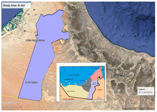
Figure 1.
Location map of Al Ain city (Google Map, 2014).
Al-Ain City experiences an arid climate characterized by consistently high temperatures throughout the year. In the winter season, temperatures typically range from 10 °C to 30 °C and rarely drop below 10 °C. Conversely, during the summer season, temperatures can soar to as high as 50 °C. Rainfall in the city is sporadic, primarily occurring in the winter months from November to March, with an average annual rainfall of around 100–120 mm in most parts of the Emirates. Al-Ain City specifically records a mean annual rainfall of 96.40 mm, while the relative humidity levels vary widely, from a very dry 13% to a very humid 88% throughout the year [46]. This gives Al-Ain City an advantage during the summer season, as it boasts low humidity levels, a preference for many people during this time of the year. Additionally, the city experiences wind speeds ranging from 1 m/s to 8 m/s (from light air to fresh breeze) throughout the year [47].
Currently, the groundwater wells in Al Ain play a crucial role in supplying water for the irrigation of agricultural and forestry sectors. These wells extract brackish water from depths of 20 m or more [44]. To supplement its water supply, Al Ain relies on water transmission systems that import water to the city. The region sources its drinking water from desalination plants located in Fujairah, Umm Al Nar, and Taweelah. The primary sectors that utilize this drinking water include residential, commercial, industrial, and governmental sectors.
3. Materials and Methods
In the study, the Linear Forecasting Model in IWR-MAIN software was used for projecting long-term demands of different urban water use in Al Ain city. The study focused on forecasting the future water use in Al-Ain city in two cases, namely, overall monthly water demand and sector-wise monthly water demand. The water consumption sectors in Al Ain were identified to be residential, agricultural, commercial, government, industrial, public services, and non-metered services. Modeling water demand required data collection of all water sectors in Al Ain for several years. Relevant data were collected from the Al-Ain Distribution Company (AADC) [45] and the Statistic Centre, Abu Dhabi (SCAD) [48]. These collected data were classified according to different variables such as population and consumption pattern to calibrate the linear forecast model and then to forecast water demand till the year 2030 in Al-Ain City. To accomplish this, data on water consumption patterns for seven distinct demand sectors (agricultural, residential, non-metered services, commercial, government, industrial, and public services) in Al-Ain City for a 15-year span spanning from 1998 to 2012 was sourced from AADC [45]. The available dataset primarily consisted of population figures for Al-Ain city, along with average monthly temperature and average rainfall data for each of the twelve months for the period 1998 to 2012. To analyze this dataset, the Statistical Package for Social Science (SPSS), Version 21 for Windows, was employed.
The data were analyzed statistically using analysis of variance (ANOVA). Statistical significance is achieved when a p-value is equal to or smaller than the chosen significance level (α), often set at 5%. When the p-value is less than or equal to the significance level, it leads to the rejection of the null hypothesis, which typically asserts “no difference.” In the context of this analysis, the relationship between water consumption (the dependent variable) and population size is considered statistically significant. This conclusion was drawn because the p-value is equal to 0.000, which is less than the threshold of 0.05. On the other hand, the analysis showed that water consumption is not significantly associated with temperature and rainfall. The calculated p-values for these variables were 0.394 and 0.232, respectively, which are both greater than the significance level of 0.05. Consequently, in this study, the sole independent variable considered is the population size of Al-Ain city. In summary, based on this analysis, water consumption, the dependent variable, is deemed to be significantly influenced by the population size, and thus, only the population size of Al-Ain City is utilized as the independent variable in this study.
This proposed forecasting method calculates the future water demand for each subsector in the future by considering the model intercept and the explanatory variables. The forecasted subsector water demand is determined using a linear forecasting model within IWR-MAIN, represented by Equation (1):
where:
= Estimated daily use rate per unit in subsector (s) in the month (m) in the base year (y).
α = Model intercept for subsector (s) in the month (m).
X = Value of explanatory variable (j) in subsector (s) in month (m).
β = Coefficient of per unit use for a variable (j) in subsector (s) in month (m).
Then, the estimated daily use rate per unit per day for the month (q) was then multiplied by the number of units (N) and by the number of days in the month to determine the sub-sector demand as given in Equation (2):
where:
Q = Cubic meters of water used in sector (s) in the month (m) in year (y).
N = Number of units in subsector (s) in month (m) in year (y).
q = Average daily use rate per unit in subsector (s) in the month (m) in base year (b).
d = Number of days in the month (m).
The next step in the calibration process was to compare the actual water use and simulated water demand of all selected base years. The calibration with minimum simulated error was used in the forecast scenarios. Equations (3)–(6) depict how the error calculations were performed for each of the calibration simulations. These calculations encompass the Absolute Relative Error (AREi), the Average Absolute Relative Error (AARE), the Standard Deviation of the Absolute Relative Error (SDARE), and the Average Root Mean Square Error (ARMSE).
where:
CDi is the calibrated demand of year i of the calibration period.
ADi is the actual demand of year i of the calibration period.
n is the number of years in the calibration period.
In the study, for the linear forecasting model, the rate of water use per unit () for the base year was computed by dividing the base year water use by the number of counting units in each subsector. This calculated rate of water use remains constant for all forecast years within each subsector. To project the water, use for each subsector in future years, this rate () (cubic meters per unit per day) is multiplied by the forecasted counting units, and the result is then multiplied by the number of days in the specified month (dm). This process yields the estimated water demand () for the given subsector (s), month (m), and year (y), with the use rate expressed in cubic meters per unit per day.
The Forecast Manager within the IWR-MAIN program was employed to project the water demand in Al Ain City for the years leading up to 2030. The study categorizes the forecasted results into three main classifications: (i) the overall yearly demand, (ii) the overall monthly demand, and (iii) the sector-wise yearly water demands.
4. Results and Discussion
The IWR-MAIN Specify Forecasting Linear Model is calibrated using available data. In the calibration process, multiple simulations were conducted using different base years to identify the base year that most accurately represents the demand. Once this optimal base year was determined, it was then used as the basis for making the forecast. The calibration process was conducted independently for both the overall monthly water demand and sector-wise monthly water consumption. Throughout the calibration period, SPSS was utilized to calculate the values of intercepts and coefficients. These determined intercepts and coefficients were subsequently integrated into the IWR-MAIN software for the purpose of water demand forecasting.
4.1. Model Calibration for Overall Annual Water Demand
Before utilizing the program, the model’s explanatory coefficient and intercept were determined through the use of SPSS. In this particular study, the sole explanatory variable for estimating the overall annual demand is the population size of Al-Ain City. The intercept and coefficient values (α, β) were derived from SPSS, resulting in estimated values of α = −16,585.61646 and β = 0.122673 for the overall annual demand forecast.
Using the linear forecasting model, changes in estimated water usage from year to year for different sectors are attributed to alterations in the explanatory variables. Thirteen distinct simulations were executed, each employing different base years, to pinpoint the base year that provides a more accurate representation of water demand. Figure 2 depicts the comparison between actual and simulated overall water usage in a million cubic meters per year (MCMY) using different base years (B 1998 to B 2010) for the calibration period spanning from 1998 to 2012, using the historical water consumption data. The actual water consumption generally exhibits an upward trend over time, with the exception of a decrease in 2010. The exception of the water consumption trend of 2010 can be attributed to the reduction in the expat population because of the economic crisis that affected the entire world. The highest actual water usage occurs in the year 2012. Notably, all calibration simulations depict a gradual increase in water demand throughout the calibration period.
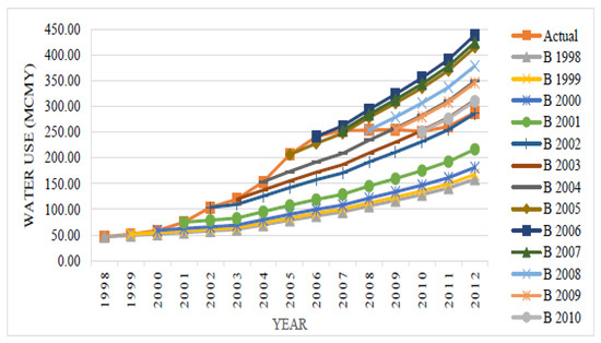
Figure 2.
Actual and simulated overall annual water demand.
The AARE, SDARE, and ARMSE were computed using Equations (3)–(5) for each calibration simulation. Figure 3 illustrates that the error values tend to increase in later base years (2005–2008). This increase is primarily due to fluctuations in actual water usage in the later years, leading to differences between the actual and simulated water usage. Interestingly, the simulation based on the year 2010 exhibits the lowest errors in comparison to other years. Therefore, the calibration simulation utilizing the base year 2010 has been selected for forecasting water demand scenarios in this model.
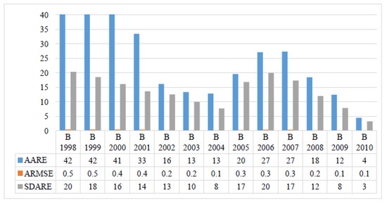
Figure 3.
Error-values of all calibration simulations for overall annual water demand.
4.2. Model Calibration for Overall Monthly Water Demand
Figure 4 shows the monthly water use data in million cubic meters for the period 1998–2012, comparing the actual values with those simulated using the IWR-MAIN program. Throughout the calibration period, SPSS was utilized to determine the intercepts and coefficients for the independent variables, as outlined in Equation (1), utilizing historical water consumption data. Table 1 provides the coefficients and intercepts (β, α) for overall monthly water demands, which were derived from SPSS.
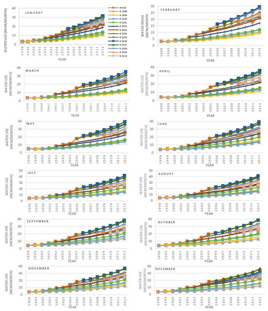
Figure 4.
Actual and simulated monthly water demand based on different base years.

Table 1.
Explanatory coefficients and intercepts (β, α) for overall monthly water demand.
The historical water consumption trends, indicating a general increase over time with some exceptions during specific months in 2010 and 2011, are shown in Figure 4. The highest overall consumption was recorded in the year 2012, with the peak monthly consumption observed in July of the same year. July typically coincides with the hottest temperatures (with an average of 38 °C) in Al-Ain, which results in a substantial increase in water usage, especially for cooling and other purposes [45]. Conversely, the lowest monthly consumption is observed in February. This can be attributed to the fact that February is a rainy month in Al-Ain City, with an average precipitation of 4.3 mm [48]. The presence of rainfall reduces the demand for irrigation water, contributing to the overall decrease in water consumption during this month. Additionally, the absolute temperature in February tends to be lower, with an average of 21 °C in the year 2012 [45], further contributing to the lower total water consumption during that period.
The values of each base year were employed to simulate water demand over the calibration period, and subsequently, the simulated results were compared to the actual demand. The base year that demonstrated the least disparities between simulated and actual water demand was chosen for forecasting future water demands. Error-values are computed for each calibration simulation, and Figure 5 provides a summary of the calculated values of AARE, ARMSE, and SDARE for all calibration simulations utilizing different base years. This analysis helped to identify the most accurate base year for forecasting purposes.
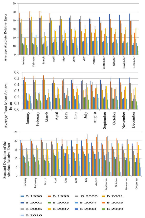
Figure 5.
Error-values of all calibration simulations for overall monthly water demand.
The simulations using the base year 1999 showed the highest AARE and ARMSE values for the initial four months, whereas the simulations using the base year 2000 exhibited these highest values for the months of May, June, and July. Notably, for the last five months of the base year, 1998 simulations showed the highest AARE and ARMSE. The simulations based on the base year 1998 exhibited the highest SDARE values for the initial three months of the year (Figure 5). In contrast, May of 1999 recorded the highest SDARE, while October and December, based on the base year 2005, exhibited the highest SDARE values. For the remaining six months, the simulations utilizing the base year 2006 showed the highest SDARE. Applying the same criteria employed during the calibration of overall annual water demand, Table 2 presents the optimal base year for each month, which was taken into account for the forecasting scenarios.
Table 2.
Best base years for monthly water demand.
4.3. Model Calibration of Sector-Wise Monthly Water Demand
Therefore, the calibration of monthly water demand for seven sectors was performed using different base years. To facilitate the presentation of results, each sector is individually discussed below. In Table 3, the model coefficients and intercepts (β, α) acquired through the SPSS program for each sector are included.
Table 3.
Explanatory coefficients and intercepts (β, α).
4.3.1. Agricultural Sector
The graphical representation of the actual and simulated monthly water usage for the agricultural sector over twelve months, considering various base years, is shown in Figure 6. The figure highlights that the peak actual water consumption occurred in 2012. Notably, within that year, the highest monthly water consumption was recorded in October, having an average temperature of 31 °C [45].
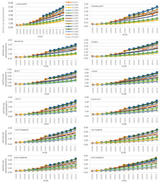
Figure 6.
Actual and simulated monthly water use for the agricultural sector.
The AARE, ARMSE, and SDARE for all simulated base years are depicted in Figure 7 for the 12 months of the year. It can be observed that the highest AARE and ARMSE for the first four months of the year are exhibited by the simulation of the base year 1999. The base year 2000 showed the highest AARE and ARMSE for the months of May, June, and July; however, the highest AARE and ARMSE for the last five months of the year were obtained by the simulation of the base year 1998. The first three months got the highest SDARE for the base year 1998, while the highest SDARE for May was recorded in the base year 1999. October and November exhibited the highest SDARE values in the base year 2005, while the other months showed this pattern in the base year 2006. Utilizing the same criteria to select the most suitable base year, the months of April and the last six months of the year demonstrated the least AARE and ARMSE when using the base year 2010. However, the minimum SDARE, considering a longer calibration period, is achieved for March, May, and June with the base year 2009, whereas the base year 2004 is optimal for the months of January and February.
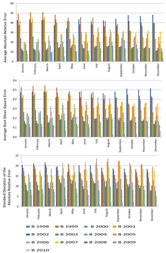
Figure 7.
Error-values of all calibration simulations for the agricultural sector.
4.3.2. Residential Sector
The actual and simulated monthly water usage for the residential sector using various base years is illustrated in Figure 8. It is evident that the highest actual consumption was observed in 2012, with the highest monthly consumption recorded in March, characterized by an average temperature of 24 °C and average precipitation of around 0.5 mm. Conversely, the lowest monthly consumption was noted in February, with an average temperature of 21 °C and average precipitation of approximately 4.3 mm [45,48].
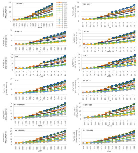
Figure 8.
Actual and simulated monthly water use for the residential sector.
The calculated AARE, ARMSE, and SDARE for all calibration simulations across the twelve months of the year are presented in Figure 9. Figure 9 was also employed to select the best base year for forecasting water demand for specific months. The results indicated that the base year 2010 is best for April and the last six months of the year, while March, May, and June are best with the base year 2009, and the months of January and February are best with the base year 2004.
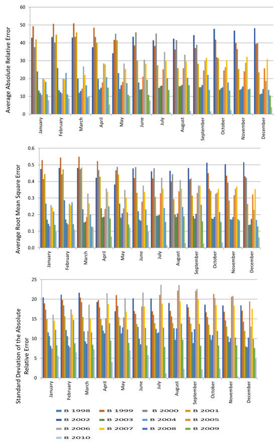
Figure 9.
Error-values of all calibration simulations for the residential sector.
4.3.3. Government Sector
The actual and simulated monthly water use for the government sector is displayed in Figure 10. In 2012, the highest actual consumption was observed in August (with an average temperature of 37 °C), while the lowest actual consumption was recorded in March (with an average temperature of 24 °C) [45].
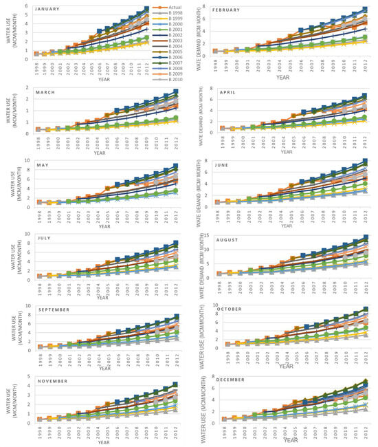
Figure 10.
Actual and simulated monthly water use for the government sector.
The values of AARE, ARMSE, and SDARE for all calibration simulations are shown in Figure 11. The year 2010 is identified as the best base year for forecasting future demand in April and the last six months of the year. Meanwhile, the year 2009 is determined to be the most suitable base year for March, May, and June, while the year 2004 is considered the best for January and February.
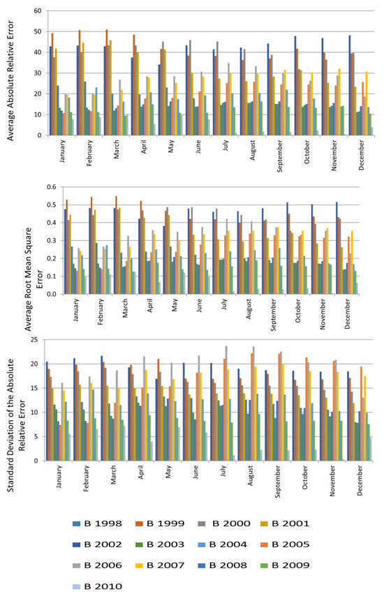
Figure 11.
Error-values of all calibration simulations for the government sector.
4.3.4. Other Sectors
The other four sectors, namely the non-metered services sector (services without a water meter to measure usage), commercial sector, industrial sector, and public services sector, underwent an analysis. In the non-metered services sector, the results indicate that the highest and lowest actual consumption occurred in the year 2012 during the months of August (with an average temperature of 37 °C) and February (with a low average temperature of 21 °C), respectively [45].
In the commercial sector, the results showed that the highest actual consumption occurred in August (with an average temperature of 37 °C) in the year 2012, while the lowest actual consumption was observed in February (with an average temperature of 21 °C) in the same year [45].
In the industrial sector, the results indicated that the highest actual consumption was observed in June of the year 2012, characterized by high temperatures (with an average of 35 °C) and minimal rainfall (with an average of 0.0 mm). Conversely, the lowest actual consumption was recorded in the same year in February, a month with lower temperatures (averaging 21 °C) and increased rainfall (with an average of around 4.3 mm) [45,48].
The simulation results for the public services sector indicate that the highest and lowest actual consumption occurred in the year 2012, with the highest consumption in April (with an average temperature of 30 °C) and the lowest consumption in February (with an average temperature of 21 °C) [45]. Figure 12, Figure 13 and Figure 14 represent the calculated AARE, ARMSE, and SDARE, respectively, for all calibration simulations for the four sectors.
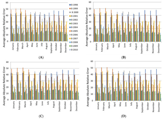
Figure 12.
The AARE values of all calibration simulations for (A) non-metered services, (B) commercial, (C) industrial, and (D) public services.
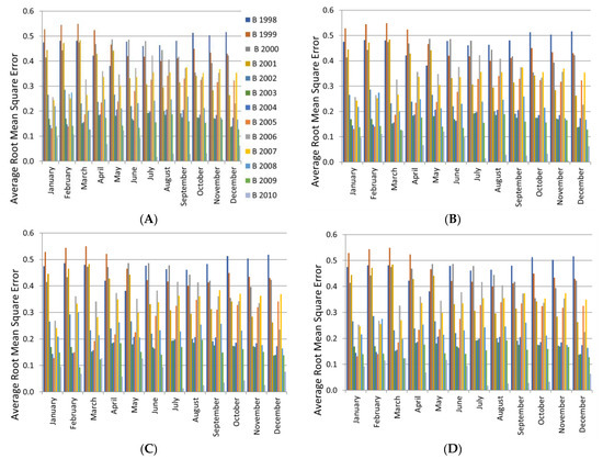
Figure 13.
The ARMSE values of all calibration simulations for (A) non-metered services, (B) commercial, (C) industrial, and (D) public services.
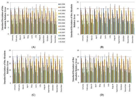
Figure 14.
The SDARE values of all calibration simulations for (A) non-metered services, (B) commercial, (C) industrial, and (D) public services.
The results from Figure 12, Figure 13 and Figure 14 indicate that for the non-metered services sector, the base year 2010 is best for April and the last six months of the year. The base year 2009 is selected for March, May, and June, while the base year 2004 is chosen for the months of January and February. In the case of the commercial sector, the results suggest that the base year 2010 is suitable for April and the last six months of the year. For March, May, and June, the best base year is 2009, while January and February are best represented by the base year 2004. Figure 12, Figure 13 and Figure 14 also reveal that for the industrial sector, the base year 2010 is appropriate for April, May, and the last six months of the year. However, for March and June, the calibration simulation with the base year 2009 is selected, and the base years 2004 and 2005 are chosen for January and February, respectively. Lastly, for the public services sector, the base year 2010 is recommended for April and the last six months of the year. March, May, and June are best represented by the base year 2009, while January and February are accurately captured by the base year 2004. Table 4 summarizes the best base year for monthly water use for each sector that will be considered for the forecasting scenarios.
Table 4.
Sector-wise, the best base year for demand forecast.
4.4. Model Verification
The purpose of model verification is to ensure the accuracy of the model’s implementation. In this study, verification was carried out using data from the years 2009 to 2012 out of the total available data spanning from 1998 to 2012. Two different base years, 2008 and 2010, were employed for model verification. The results clearly demonstrated that the optimal base year for forecasting water demand is 2010, consistent with the findings from model calibration. These results, as shown in Figure 15, provided assurance regarding the correct implementation of the IWR-MAIN program, and were subsequently utilized to simulate various water demand scenarios. It is noteworthy that the average errors did not exceed 3% when comparing the model’s output to the actual data, affirming the model’s reliability.
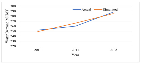
Figure 15.
Actual and simulated values for the years 2010–2012 for verification of the model with the base year 2010.
4.5. Water Scenarios Development
Demand forecasting involves the process of estimating future water demand. Scenarios play a crucial role in helping decision-makers explore various options, anticipate potential developments, and formulate new strategies. The Forecast Manager within the IWR-MAIN program is a valuable tool that can assist water planners in projecting future water demands under different scenarios. Indeed, the future water demand in Al Ain city is influenced by a multitude of factors, including population growth, urbanization trends, improvements in living standards, income levels, and more. The Al-Ain 2030 plan outlines a vision for the city’s future development, with a strong emphasis on achieving sustainability across environmental, economic, cultural, and social dimensions. To align with this vision and support the goal of water sustainability, this study has developed scenarios to explore and anticipate the city’s future water demand. These scenarios provide valuable insights for effective water resource management and planning, ensuring that Al Ain can thrive while maintaining a sustainable and balanced approach to its development. Nonetheless, in order to maintain an equilibrium between development and conservation, the Al-Ain 2030 strategy aims to foster genuine Arabic cultural heritage while also supporting the progression toward a more contemporary nation [49]. Additionally, the future development of Al-Ain City involves strategies to enhance renewable water sources and reduce the utilization of non-renewable water resources [50].
Population growth, governmental policies, and other external drivers, such as water loss, served as the foundation for the scenario development in Al Ain. Two clusters of scenarios are developed. Namely, population-tied scenarios and water loss impact scenarios.
4.5.1. Population-Tied Scenarios
In the suite of Population-tied Scenarios, a reference scenario named Baseline Water Scenario, and four other sub-scenarios named Moderate Population Growth (MPG) water scenario, Megaprojects (MP) water scenario, Tourism Focused (TF) water scenario and High Population Growth (HPG) water scenario were developed to study the change in water demands of Al Ain. Figure 16 illustrates the population projections for the various scenarios.
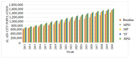
Figure 16.
Population forecast of Al Ain city for different scenarios.
Base Water Scenario
A plausible future water demand scenario was developed for Al Ain, considering the natural population growth of Al Ain. For the scenario named as the base scenario, the expected population growth in Al Ain was considered to grow exponentially rather than linearly. By 2030, it is projected that the population will nearly double. According to the Urban Structure Framework Plan [48], the population of Al Ain city in the year 2005 stood at 338,970. By the baseline year of 2007, the population had grown to 374,000, with an annual tourist visitation rate of 200,000 in that same year. Therefore, the population of Al Ain was predicted using exponential regression in SPSS based on the available data, as shown in Figure 16.
Moderate Population Growth Water Scenario
The MPG scenario explores the impact of moderate population growth on water demand in Al Ain city. This scenario envisions a population size for residents in 2030 that is approximately 8% higher than the population size expected in the base scenario (Figure 16). This scenario assumes that all essential factors and elements remain the same as in the base year, with socioeconomic and demographic parameters growing at the officially anticipated rate. Within this scenario, it is assumed that water usage remains sustainable, with a medium percentage change that is higher than that of the base scenario.
Megaprojects Water Scenario
The MP scenario examines the potential impact of immigration to fulfill the labor needs for expected megaprojects in Al Ain city. In a world characterized by continuous progress, cities aim for advanced technology and a very high standard of living through the development of megaprojects and industries. This scenario places a strong emphasis on market solutions and globalization, which suggests that cities will likely experience significant migration. Accordingly, this scenario was designed to assess the trend in water demand in Al Ain resulting from a potential increase in immigrants to the city. Given the UAE government’s emphasis on security and the implementation of barriers, we assumed a moderate level of migration to Al Ain, primarily driven by improved access to high-quality education and healthcare services, which are part of the megaprojects planned for Al Ain.
Tourism-Focused Water Scenario
The TF scenario took into account the expected visitors to Al-Ain city, which includes the population size derived from the Megaprojects scenario, as well as the number of tourists expected to spend two to four weeks in Al-Ain. Al-Ain city boasts a wide range of tourist attractions, including Al Ain Museum, Al Ain Zoo, Ain Al Fayda Resort, and Al Hili Fun City. In this scenario, as tourism continues to grow in Al Ain, the city experiences the emergence of a middle class.
High Population Growth Water Scenario
The HPG scenario takes into account the impacts of population growth resulting from various plausible causes, including tourism, immigration, and megaprojects. This sub-scenario considers a high population growth rate without a balanced focus on environmental and economic growth rates. This is achieved by assuming high economic growth rates, as outlined in The Abu Dhabi Water Strategy [51], which would result in higher immigration rates of workers into Al Ain.
4.5.2. Water Loss Scenarios
One of the major external drivers of water demand is the significant water losses occurring in the distribution network system, making it challenging to quantify these losses accurately. These water losses are categorized into two main groups: losses stemming from pipe networks and ad losses resulting from illegal connections and government-subsidized water. Data obtained from the Al-Ain Distribution Company [45] indicated that losses within the water distribution system of Al Ain City account for approximately 20%. In the broader context, the UAE addresses its potable water deficit by supplying desalinated water [48]. Therefore, accounting for water loss is essential when estimating water demand. It is crucial to reduce the volume of lost water, as numerous studies have highlighted the environmental consequences of desalination plants in the Arabian Gulf [26]. Hence, effective management of desalinated water supply is vital for the long-term water resource development of the region. Consequently, this study considers water loss in the distribution system of desalinated water to create a range of water scenarios, aiming to assess their impact on overall water demand. These scenarios investigate the effects of gradually increasing the percentage of lost water from the current 20%.
4.6. Simulation Results for Population-Tied Water Scenarios
The simulation results from IWR-MAIN for the population-tied water scenarios are discussed in this section.
4.6.1. Overall Annual Water Demand
The total annual water demand forecast from 2013 to 2030 (in million cubic meters per year) is presented in Figure 17. It shows that the simulated result depends on the model coefficient and intercept (β, α) that depends on the population growth. By 2030, the estimated annual demand will reach 722 million cubic meters per year, and the water demand increase will be around 46% by 2030 as compared to 2012.
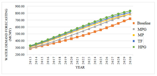
Figure 17.
Al-Ain City forecast overall annual water demand for population-tied scenarios.
Furthermore, a comparison of yearly water demands for other water scenarios that were developed was carried out. It is evident from Figure 17 that changes in water demand projections are directly correlated with changes in the population size. In general, water demand is projected to increase by 1.5%, 2%, and 2.5% in 2020, 2025, and 2030, respectively, compared to water use in 2013. Additionally, Figure 17 illustrates that the difference between the baseline scenario and the MPG water scenario is nearly 10% and 8% in 2020 and 2030, respectively. Scenario 2’s water demand projection indicates that mega-developments will require 16.5% more water than the base scenario in 2020 due to the increased number of workers, and this demand will decrease to 8% in 2030 as construction work concludes. The HPG water scenario shows a 2.8% increase in water demand compared to the TF water scenario.
4.6.2. Overall Monthly Water Demand
This simulation was aimed to identify the month with the highest water demand in Al Ain. The simulation results for the baseline scenario carried out until the year 2030 are depicted in Figure 18. It is evident that the months of August and September exhibit the highest water demand. August records the highest water demand from 2013 to 2025, while September surpasses it from 2026 to 2030. Conversely, June consistently has the lowest water demand in the majority of years within the study period.
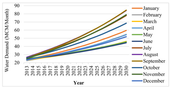
Figure 18.
Overall Monthly water demand forecasted for the baseline scenario.
4.6.3. Sector-Wise Monthly Water Demand Forecast
The monthly water demand forecasts for seven sectors considered in the study in Al Ain are shown in Figure 19. The simulations of the Linear Forecasting Model are dependent on the model’s intercept and coefficient (α, β). As a result, the water demand for certain months does not consistently increase over the years. In Figure 19, it is evident that the agricultural sector exhibits the highest water demand in October, while April shows the lowest demand. Both the commercial and government sectors experienced their peak water demand in August. On the other hand, the government sector has the lowest demand in March, while the commercial sector has its lowest demand in February from 2013 to 2023 and in May from 2024 to 2030. November witnessed the most significant increase in water demand for the residential and public services sectors. The non-metered services sector shows the lowest water demand from June 2017 to 2030 and the highest demand in August. As for the industrial sector, June and August have the lowest estimated water demand during the periods of 2013–2021 and 2022–2030, respectively, with the least amount of water required in February. Figure 19 also illustrates that for the government and industrial sectors, the months with the lowest demand, March and February, respectively, maintain a relatively constant pattern.
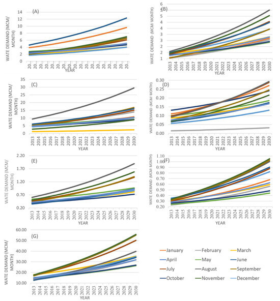
Figure 19.
Monthly water demand forecast for (A) agricultural, (B) commercial, (C) government, (D) industrial, (E) non-metered services, (F) public services, and (G) residential.
A simulation was conducted to determine the month with the highest water demand in Al Ain. The simulation results for the baseline scenario carried out until the year 2030 are presented in Figure 18. It is evident that the months of August and September consistently have the highest water demand. Specifically, August exhibits the highest water demand from 2013 to 2025, while September takes over as the month with the highest demand from 2026 to 2030. Conversely, June consistently has the lowest water demand for the majority of the years in the study period.
4.7. Simulation Results for Water Loss Scenarios
Three sub-scenarios, namely, Low Loss (LL), Medium Loss (ML), and High Loss (ML) were simulated. The water loss was assumed to reach 25%, 30%, and 35% of the total water production for the scenarios LL, ML, and HL, respectively. Therefore, in IWR-MAIN, the expected percentages of lost/ unaccounted water were entered for the forecasting years. Figure 20 shows the comparison of the water demands as simulated by the model.
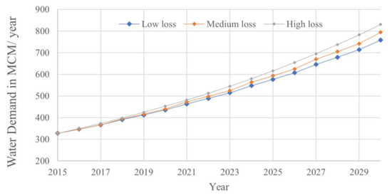
Figure 20.
Simulated overall annual water demand for the water loss scenarios.
Figure 20 illustrates the increase in total water demand across three scenarios over the years. As previously mentioned, the IWR-MAIN program computes losses based on provided values. Consequently, as long as loss percentages continue to rise in all projected years, the total water demand (comprising metered, unmetered, and losses) will also continue to climb. Figure 20 unmistakably highlights that the total demand in the HL scenarios surpasses that of the other two scenarios, with the difference becoming more pronounced as it approaches 2030.
5. Conclusions
This study has provided water demand predictions for Al-Ain city till year 2030. The research utilized various available databases across different water use sectors, population size, average temperature, and average rainfall. Through simulations conducted with the SPSS program, it was determined that population size is the sole significant independent variable in this study, whereas average temperature and rainfall amount did not exhibit significant correlations with water consumption. The calibration and prediction of the Linear Forecasting Model were carried out in this study using the IWR-MAIN program. This model relies on population size, model coefficient (β), and model intercept (α). Calibration of the model involved the utilization of two datasets: total monthly water usage and monthly water usage for seven distinct sectors. These sectors encompass agricultural, residential, non-metered services, commercial, government, industrial, and public services.
Several factors contribute to uncertainties in the provided data by AADC, including uncertainties in reading and recording procedures. For instance, if a reading was not taken for a specific month, an average consumption reading is often used. It is important to note that the uncertainty in projected water demand tends to rise as the projection period increases. Additionally, the uncertainty in forecasting water demand is intrinsically linked to the prediction of population growth. As a result, the accuracy of the assumptions made plays a crucial role in determining the reliability of the results.
The results indicate that the peak water demand takes place in August until 2025 and then shifts to September from 2026 to 2030. Additionally, the agricultural sector experienced its highest water demand in October. As for the commercial and government sectors, their highest water demand is anticipated in August. Furthermore, the industrial sector is projected to have the lowest water demand in the month of August until 2030.
To achieve the necessary supply for water demand outlined in each scenario, it is crucial to implement specific programs. Regulations and water conservation alone will not suffice to reach these goals unless there is a recognition of the necessity for change. The potential for integrating water supply and renewable energy sources in Abu Dhabi to enhance sustainability has to be explored. In this context, the integration refers to the use of renewable energy technologies to power water supply and treatment processes, making them more environmentally friendly and efficient. By integrating renewable energy into water supply and treatment processes, the UAE can reduce its reliance on fossil fuels, decrease greenhouse gas emissions, and move towards a more sustainable and environmentally friendly water management system. This not only benefits the environment but also enhances the long-term resilience of the water supply in the face of climate change and resource constraints.
Author Contributions
Conceptualization, M.M.M. and H.I.Y.; Data curation: H.I.Y.; Formal analysis: M.M.M. and H.I.Y.; Funding acquisition: M.M.M.; Investigation: M.M.M. and H.I.Y.; Methodology: M.M.M. and H.I.Y.; Software: H.I.Y.; Validation: M.M.M. and M.I.K.; Writing—original draft, H.I.Y.; Review and editing, M.M.M. and M.I.K. All authors have read and agreed to the published version of the manuscript.
Funding
This research was funded by the national water and energy center, United Arab Emirates University, through the Asian University Alliance (AUA) program, grants number 12R176-AUA-NWEC-4-2023. Initial results of this work was supported by the UAE National Research Foundation under the university-industry research collaboration program [grant number UIRCA 24826].
Data Availability Statement
The datasets generated during and/or analyzed during the current study are available from the corresponding author upon reasonable request.
Conflicts of Interest
The authors declare no conflict of interest.
References
- Billings, R.B.; Jones, C.V. Forecasting Urban Water Demand; American Water Works Association: Denver, CO, USA, 2008. [Google Scholar]
- Armstrong, J.S.; Fildes, R. Making progress in forecasting. Int. J. Forecast. 2006, 22, 433–441. [Google Scholar] [CrossRef]
- Proskuryakova, L.N.; Saritas, O.; Sivaev, S. Global Water Trends and Future Scenarios for Sustainable Development: The Case of Russia. J. Clean. Prod. 2018, 170, 867–879. [Google Scholar] [CrossRef]
- Rinaudo, J.-D. Long-Term Water Demand Forecasting. In Understanding and Managing Urban Water in Transition; Grafton, Q., Daniell, K.A., Nauges, C., Rinaudo, J.-D., Chan, N.W.W., Eds.; Springer: Dordrecht, The Netherlands, 2015; pp. 239–268. [Google Scholar]
- Almutaz, I.; Ajbar, A.; Khalid, Y.; Ali, E. A probabilistic forecast of water demand for a tourist and desalination dependent city: Case of Mecca, Saudi Arabia. Desalination 2012, 294, 53–59. [Google Scholar] [CrossRef]
- Cresswell, M.; Naser, G. Forecasting Water Demands—A Case Study for the South East Kelowna Irrigation District. In World Environmental and Water Resources Congress 2012; American Society of Civil Engineers: Reston, VA, USA, 2014; pp. 2739–2747. [Google Scholar]
- Donkor Emmanuel, A.; Mazzuchi Thomas, A.; Soyer, R.; Alan Roberson, J. Urban Water Demand Forecasting: Review of Methods and Models. J. Water Resour. Plan. Manag. 2014, 140, 146–159. [Google Scholar] [CrossRef]
- Zhou, S.L.; McMahon, T.A.; Walton, A.; Lewis, J. Forecasting daily urban water demand: A case study of Melbourne. J. Hydrol. 2000, 236, 153–164. [Google Scholar] [CrossRef]
- Ajbar, A.; Ali, E.M. Prediction of municipal water production in touristic Mecca City in Saudi Arabia using neural networks. J. King Saud Univ. Eng. Sci. 2015, 27, 83–91. [Google Scholar] [CrossRef]
- Bennett, C.; Stewart, R.A.; Beal, C.D. ANN-based residential water end-use demand forecasting model. Expert Syst. Appl. 2013, 40, 1014–1023. [Google Scholar] [CrossRef]
- Ghiassi, M.; Fa’Al, F.; Abrishamchi, A. Large metropolitan water demand forecasting using DAN2, FTDNN, and KNN models: A case study of the city of Tehran, Iran. Urban Water J. 2017, 14, 655–659. [Google Scholar] [CrossRef]
- Dziegielewski, B.; Baumann, D.D. Tapping Alternatives: The Benefits of Managing Urban Water Demands. Environ. Sci. Policy Sustain. Dev. 1992, 34, 6. [Google Scholar] [CrossRef]
- Lowry, J.H.; Ramsey, R.D.; Kjelgren, R.K. Predicting urban forest growth and its impact on residential landscape water demand in a semiarid urban environment. Urban For. Urban Green. 2011, 10, 193–204. [Google Scholar] [CrossRef]
- Mohamed, M.M.; Al-Mualla, A.A. Water demand forecasting in Umm Al-Quwain using the constant rate model. Desalination 2010, 259, 161–168. [Google Scholar] [CrossRef]
- Altunkaynak, A.; Özger, M.; Çakmakci, M. Water Consumption Prediction of Istanbul City by Using Fuzzy Logic Approach. Water Resour Manag. 2005, 19, 641–654. [Google Scholar] [CrossRef]
- Mitrică, B.; Bogardi, I.; Mitrică, E.; Mocanu, I.; Minciună, M. A forecast of public water scarcity on Leu-Rotunda Plain, Romania, for the end of the 21st century. Nor. Geogr. Tidsskr.-Nor. J. Geogr. 2017, 71, 12–29. [Google Scholar] [CrossRef]
- Tabesh, M.; Dini, M. Fuzzy and neuro-fuzzy models for short-term water demand forecasting in Tehran. Iranian J. of Sci. Tech. Trans. B Eng. 2009, 33, 18. [Google Scholar]
- Chen, G.; Long, T.; Bai, Y.; Zhang, J. A Forecasting Framework Based on Kalman Filter Integrated Multivariate Local Polynomial Regression: Application to Urban Water Demand. Neural Process. Lett. 2019, 50, 497–513. [Google Scholar] [CrossRef]
- Nasseri, M.; Moeini, A.; Tabesh, M. Forecasting monthly urban water demand using Extended Kalman Filter and Genetic Programming. Expert Syst. Appl. 2011, 38, 7387–7395. [Google Scholar] [CrossRef]
- Wang, X.; Babovic, V. Application of hybrid Kalman filter for improving water level forecast. J. Hydroinform. 2016, 18, 773–790. [Google Scholar] [CrossRef]
- Peña-Guzmán, C.; Melgarejo, J.; Prats, D. Forecasting Water Demand in Residential, Commercial, and Industrial Zones in Bogotá, Colombia, Using Least-Squares Support Vector Machines. Math. Probl. Eng. 2016, 2016, 5712347. [Google Scholar] [CrossRef]
- Kim, J.H.; Hwang, S.H.; Shin, H.S. A neuro-genetic approach for daily water demand forecasting. KSCE J. Civ. Eng. 2001, 5, 281–288. [Google Scholar] [CrossRef]
- Msiza, I.S.; Nelwamondo, F.V.; Marwala, T. Artificial Neural Networks and Support Vector Machines for water demand time series forecasting. In Proceedings of the 2007 IEEE International Conference on Systems, Man and Cybernetics, Montreal, QC, Canada, 7–10 October 2007; pp. 638–643. [Google Scholar]
- Pulido-Calvo, I.; Gutiérrez-Estrada, J.C. Improved irrigation water demand forecasting using a soft-computing hybrid model. Biosyst. Eng. 2009, 102, 202–218. [Google Scholar] [CrossRef]
- Hillier, F.; Lieberman, G. Introduction to Operations Research, 7th ed.; MacGraw Hill: New York, NY, USA, 2001. [Google Scholar]
- Al-Zubari, W. Water Resource Management Challenges in the GCC Countries: Four Scenarios. In Exploiting Natural Resources: Growth, Instability, and Conflict in the Middle East and Asia; The Henry L. Stimson Center: Washington, DC, USA, 2009; pp. 3–19. [Google Scholar]
- Al-Rashed, M.F.; Sherif, M.M. Water Resources in the GCC Countries: An Overview. Water Resour. Manag. 2000, 14, 59–75. [Google Scholar] [CrossRef]
- Peck, M.C. The A to Z of the Gulf Arab States; Scarecrow Press: Lanham, MD, USA, 2010. [Google Scholar]
- Kizhisseri, M.I.; Mohamed, M.M.; El-Shorbagy, W.; Chowdhury, R.; McDonald, A. Development of a dynamic water budget model for Abu Dhabi Emirate, UAE. PLoS ONE 2021, 16, e0245140. [Google Scholar] [CrossRef] [PubMed]
- Al-Zubari, W.K. Towards the establishment of a total water cycle management and re-use program in the GCC countries. Desalination 1998, 120, 3–14. [Google Scholar] [CrossRef]
- Albannay, S.; Kazama, S.; Oguma, K.; Hashimoto, T.; Takizawa, S. Water Demand Management Based on Water Consumption 845 Data Analysis in the Emirate of Abu Dhabi. Water 2021, 13, 2827. [Google Scholar] [CrossRef]
- Kizhisseri, M.I.; Mohamed, M.M.; Hamouda, M.A. A mixed-integer optimization model for water sector planning and policy making in arid regions. Water Resour. Ind. 2022, 28, 100193. [Google Scholar] [CrossRef]
- Lindhe, A.; Rosén, L.; Johansson, P.-O.; Norberg, T. Dynamic Water Balance Modelling for Risk Assessment and Decision Support on MAR Potential in Botswana. Water 2020, 12, 721. [Google Scholar] [CrossRef]
- Mohamed, M.M.; El-Shorbagy, W.; Kizhisseri, M.I.; Chowdhury, R.; McDonald, A. Evaluation of policy scenarios for water resources planning and management in an arid region. J. Hydrol. Reg. Stud. 2020, 32, 100758. [Google Scholar] [CrossRef]
- Ibrahim Kizhisseri, M.; Mostafa Mohamed, M.; Hamouda, M.A. Prediction of Capital Cost of RO Based Desalination Plants Using Machine Learning Approach. E3S Web Conf. 2020, 158, 06001. [Google Scholar] [CrossRef]
- Mohamed, M.M.; El-shorbagy, W.; Chowdhury, R.K.; Kizhisseri, M.I.; Nawaz, R.; McDonald, A.; Tompkins, J. Developing a Dynamic Approach to Water Budgeting for the Emirate of Abu Dhabi: Final Report; Environment Agency: Abu Dhabi, United Arab Emirates, 2016. [Google Scholar]
- Kizhisseri, M.I. Development of a Decision Support System for Sustainable Water Planning in Abu Dhabi. Ph.D. Thesis, United Arab Emirates University, Al Ain, United Arab Emirates, June 2021. Available online: https://scholarworks.uaeu.ac.ae/all_dissertations/169 (accessed on 12 December 2022).
- Baumann, D. Demand Management and Urban Water Supply Planning; ASCE: Reston, VA, USA, 1987; pp. 174–196. [Google Scholar]
- Davis, W.; Rodrigo, D.; Opitz, E.; Eziegielewski, B.; Baumann, D.; Boland, J. IWR- MAIN Water U se Forecasting System Description; lWR- Report 88-R-6; U.S. Army Crops of Engineer Institute for Water Resources: Fort Belvior, VA, USA, 1988. [Google Scholar]
- Boland, J.J. Assessing Urban Water Use and the Role of Water Conservation Measures under Climate Uncertainty. Clim. Chang. 1997, 37, 157–176. [Google Scholar] [CrossRef]
- Dziegielewski, B.; Boland, J.J. Forecasting Urban Water Use: The IWR-MAIN MODEL1. JAWRA J. Am. Water Resour. Assoc. 1989, 25, 101–109. [Google Scholar] [CrossRef]
- Mohamed, M.M.; Al-Mualla, A.A. Water Demand Forecasting in Umm Al-Quwain (UAE) Using the IWR-MAIN Specify Forecasting Model. Water Resour Manag. 2010, 24, 4093–4120. [Google Scholar] [CrossRef]
- Rizk, Z.S.; Alsharhan, A.S. Water resources in the United Arab Emirates. In Developments in Water Science; Alsharhan, A.S., Wood, W.W., Eds.; Elsevier: Amsterdam, The Netherlands, 2003; pp. 245–264. [Google Scholar]
- Environment Agency—Abu Dhabi. Abu Dhabi Water Resources Master Plan; Environment Agency: Abu Dhabi, United Arab Emirates, 2009. [Google Scholar]
- Al Ain Distribution Company. Al Ain Distribution Company Report; Al Ain Distribution Company: Al Ain, United Arab Emirates, 2013. [Google Scholar]
- Murad, A.; Mahgoub, F.; Hussein, S. Hydrogeochemical Variations of Groundwater of the Northern Jabal Hafit in Eastern Part of Abu Dhabi Emirate, United Arab Emirates (UAE). IJG 2012, 3, 410–429. [Google Scholar] [CrossRef][Green Version]
- Weatherspark. Climate Condition. 2014. Available online: https://weatherspark.com/y/148887/Average-Weather-at-Al-Ain-International-Airport-United-Arab-Emirates-Year-Round (accessed on 12 December 2020).
- Statistics Centre-Abu Dhabi. Statistical Yearbook of Abu Dhabi—2015. 2015. Available online: https://www.scad.gov.abudhabi/en/pages/GeneralPublications.aspx?pubid=79&themeid=7 (accessed on 12 December 2020).
- UPC. Abu Dhabi Urban Planning Council (UPC). 2011. Available online: https://en.wikipedia.org/wiki/Abu_Dhabi_Urban_Planning_Council (accessed on 12 December 2020).
- Abu Dhabi Council for Economic Development (ADCED). 2011. Available online: https://sharaka.added.gov.ae/en/About/About-Us (accessed on 12 December 2020).
- Environment Agency-Abu Dhabi. The Water Resources Management Strategy for the Emirate of Abu Dhabi (2015–2020), Strategy and Action Plan; Environment Agency: Abu Dhabi, United Arab Emirates, 2014. [Google Scholar]


Disclaimer/Publisher’s Note: The statements, opinions and data contained in all publications are solely those of the individual author(s) and contributor(s) and not of MDPI and/or the editor(s). MDPI and/or the editor(s) disclaim responsibility for any injury to people or property resulting from any ideas, methods, instructions or products referred to in the content. |
© 2023 by the authors. Licensee MDPI, Basel, Switzerland. This article is an open access article distributed under the terms and conditions of the Creative Commons Attribution (CC BY) license (https://creativecommons.org/licenses/by/4.0/).