Abstract
An existing Boussinesq wave model, solved in a hybrid format of the finite-difference method (FDM) and finite-volume method (FVM), with good merits of stability and shock-capturing, was used as the wave driver to simulate the beach evolution under nearshore wave action. By coupling the boundary layer model, the sand transport model, and the terrain updating model, the beach evolution model is established. Based on the coupled model, the interaction process between sandbars and waves was simulated, reproducing the process of the original sand bars diminishing, new sandbars creating, and finally disappearing. At the same time, the formation and movement process of sand bars under solitary and regular waves are numerically simulated, in the breaking zone, the water bottom has a larger shear stress, which promotes the sediment activation, transport and erosion formation, and near the breaking point, the decrease of sand-carrying capacity is the main reason for the formation of sandbars, the numerical model can accurately describe the changes in the shoreline profile under wave action.
1. Introduction
In the coastal environment, sediment disturbance is mainly caused by wave action. Accurate prediction of sediment particle suspension, settling and transport requires consideration of hydrodynamic variations during the wave cycle, such as: wave boundary layer thickness, bed shear stress and energy dissipation generated by the waves (e.g., [1,2,3]). Wave nonlinearity and irregularity outside the surf zone influence the distribution of suspended sediment concentrations [4], and in the surf zone the large-scale turbulent flow structures generated by wave breaking can lift a large amount of sediment into suspension [5,6,7]. Due to the complexity of hydrodynamics and sediment movement in the nearshore, the evolution of beach profiles under wave action has long been a focus of scientific research.
Most of the available sediment transport models mainly use phase-averaged wave models, which can only approximate the short-wave effect (e.g., wave asymmetry), so there is a need to develop a model that combines a phase-resolved wave model with a detailed intra-wave sediment transport model. The Boussinesq-type (hereafter BT) models [8,9,10,11] are phase-solving and have many advantages in terms of computational efficiency and nonlinear wave interactions. There are many sophisticated versions of Boussinesq-type models (e.g., FUNWAVE, based on the equations of Wei and Kirby [12]; MIKE21 BW, based on the equations of Madsen and Srensen [13]), and the BT models have been significantly enriched and widely applied in the modelling of coastal waves and currents in complex bathymetric configurations [14,15,16]. Some of these models have been presented to couple either a one-dimensional BT wave model [17,18,19] or a two-dimensional BT wave model [20,21,22,23,24,25], with the sediment transport and morphological model presented. The results of the above studies showed that the phase-resolving coupled model is capable of reproducing the erosion and siltation changes in the shoreline profile under wave action.
To achieve high numerical efficiency, the finite-difference method (hereafter FDM) is mainly used in the BT wave models, such as the method proposed by Wei and Kirby [12] to solve fully nonlinear equations. However, the models based on FDM solvers tend to be noisy or at least weakly unstable at high wavenumbers near the grid Nyquist limit [26], which are usually stabilized by numerical filters. In addition, wave breaking and the wet–dry interface are treated empirically in the Boussinesq models, which introduces additional sources of noise and introduces some uncertainty in the computational results. These shortcomings can be overcome by using hybrid finite-volume and finite-difference schemes (e.g., [27,28,29,30]). For these hybrid schemes, the Boussinesq-type equations were written in conservation form, the convective flux terms were discretized by the finite-volume method (hereafter FVM), and the remaining terms were approximated by the FDM. When wave breaking or the wet–dry interface occurs, higher-order nonlinear and dispersive terms have less effect on the flow field, and the Boussinesq equations degenerate to nonlinear shallow water equations (NLSW) by switching off the higher-order terms. In this way, wave breaking and the wet–dry interface are treated as a bore and a local Riemann problem, respectively, which could be solved numerically using high-resolution finite-volume numerical formats [31,32].
Sediment transport models are important for studying the evolution of beach profiles. Most early sediment transport models used energy flux approaches such as the CERC equation [33]. Later, the force balance approach was more commonly used, modelling sediment transport fluxes as a function of local hydrodynamic and bed conditions, and often formulating the sediment transport rate as a function of the Shields parameter. The force balance approach is more appropriate for wave–sediment coupling. For example, Simpson and Castelltort [34] predicted the morphological changes caused by a train of long-period waves over a shallow beach. Madsen and Durham [35] investigated the effect of the subsurface horizontal pressure gradient induced by breaking waves. Young et al. [36] and Xiao et al. [37] simulated the change in shoreline profile over a fine sand beach under a breaking solitary wave. Based on the BT wave model, Sabaruddin et al. [38] coupled a sediment transport model with a bedload transport equation to validate the Bagnold-type transport equation. Francesco et al. [39] proposed a model to simulate bed evolution dynamics in coastal regions characterized by articulated morphology. Georgios et al. [40] developed a two-horizontal-dimensional composite model to simulate coastal sediment transport and bed morphology evolution, where wave asymmetry and phase lag effects were analyzed. Although many modified formulations have been proposed, many researchers still use the classical model based only on Shields parameters, such as Meyer-Peter and Müller [41] because of its simplicity and ease of use, and it is one of the most cited models.
To better predict the topographic changes in the surf zone with strong water level variations, it is particularly necessary to use a high-precision phase-resolved wave model coupled with a beach profile model to calculate the hydrodynamic and topographic changes in the surf zone. A hybrid finite-volume and finite-difference method in the numerical solution of the Boussinesq equations is shown to be a great improvement over the traditional FDM solver, which has not been used to calculate sediment transport and beach evolution.
The aim of this study was to combine an existing BT model based on the hybrid FVM/FDM scheme with a beach profile model. Meanwhile, numerical simulations of surface evolution and beach deformation over complex nearshore terrain and wave conditions were performed to validate the accuracy of the coupled model. The rest of the paper is laid out as follows. The coupled model development is detailed in Section 2, including the wave module, the boundary layer module and the morphology module. In Section 3 and Section 4, the hydrodynamic and morphological validations are briefly described, and the analysis of the experimental data and numerical results are also given, respectively. The conclusions are presented in Section 5.
2. Model Development
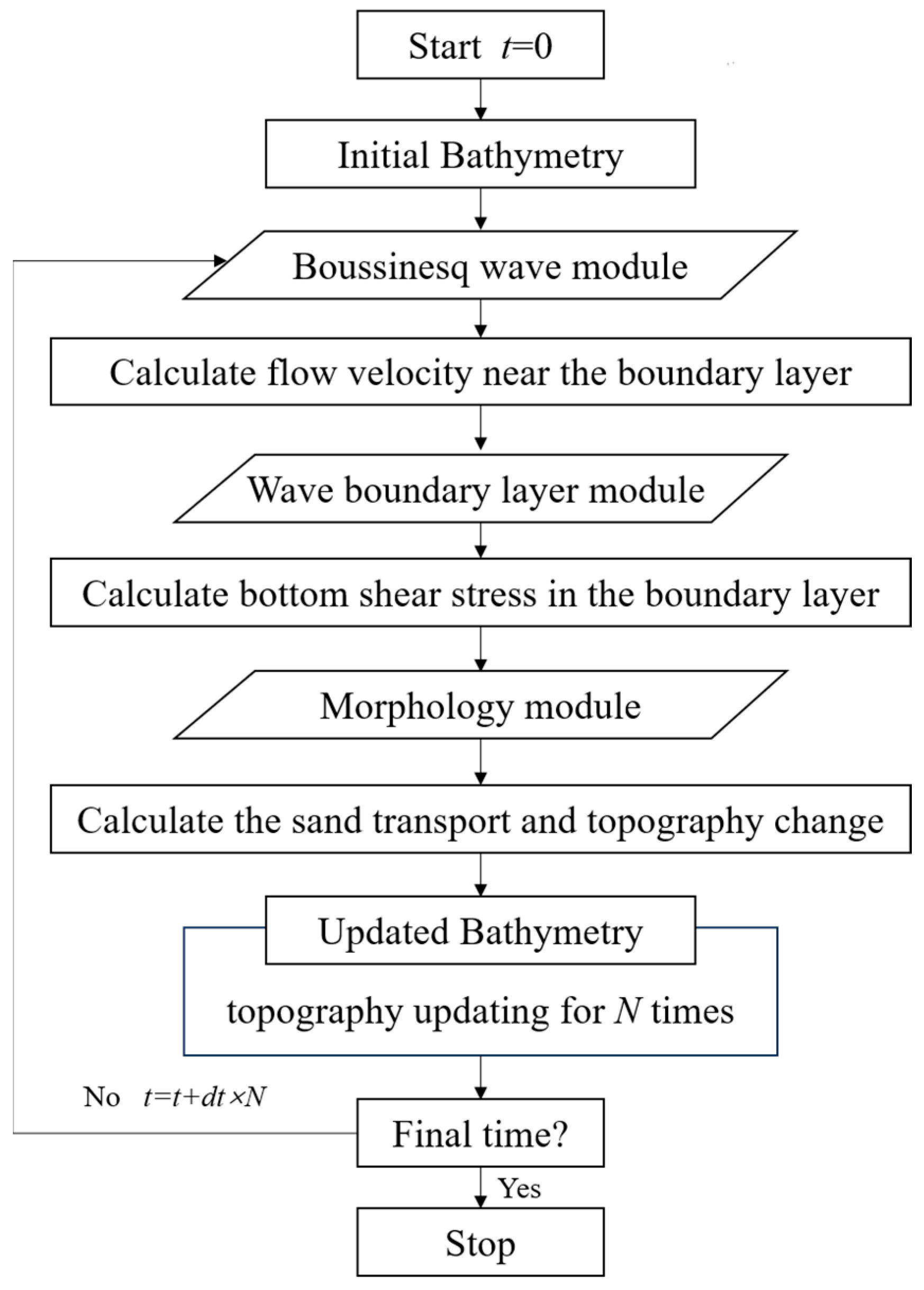
The Boussinesq wave module, the wave boundary layer module and the morphology module are dynamically integrated to predict the evolution of the beach profile. The flowchart of the coupled model is shown in Figure 1. The details of the above three modules will be given in the following subsections.
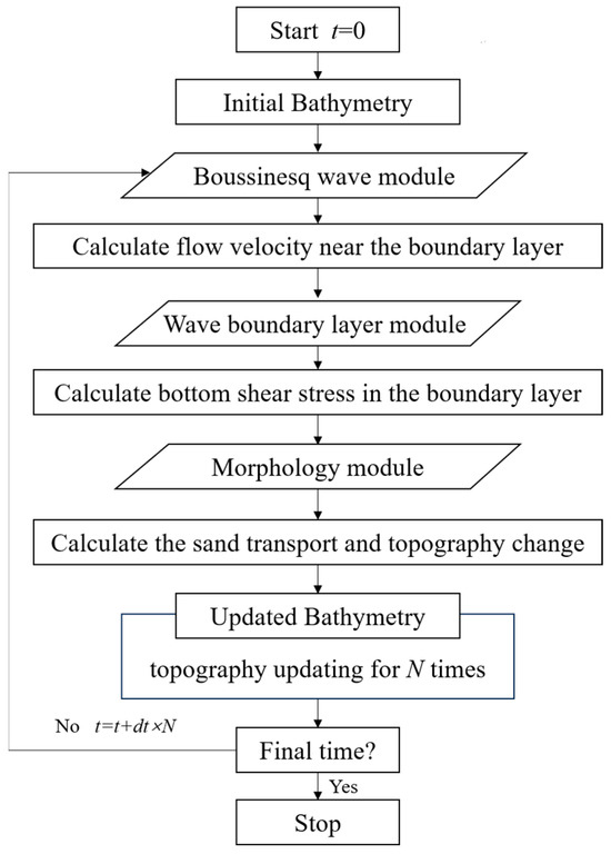
Figure 1.
Flow chart of the model.
First, the phase-resolving Boussinesq wave module is used to simulate the wave propagation process over the beach profile. The input to the wave module is the bathymetry, wave height and period, while the output is the time series of bottom velocity and other parameters related to wave breaking. Secondly, the velocity in the bottom boundary layer is computed, and the bottom shear stress is obtained by the boundary layer module. Thirdly, the calculated bottom shear stress is used to calculate the total sediment transport rate, and this instantaneous intra-wave sediment transport rate is then time-averaged to obtain the final sediment transport rate, which is finally used to update the beach profile by numerically solving the sediment conservation equation.
2.1. Wave Module
Kim et al. [42] extended the Boussinesq equation of Madsen and Sorensen [13] to obtain:
In the above equations, represents the free surface elevation measured from the still water level, represents the still water depth, is the total water depth, defined as , is the dispersive term and the subscripts x and t represent the derivative with respect to horizontal coordinate and time. The corresponding relationship of the above variables is shown in Figure 2. denotes the fluxes, is the depth-averaged velocity vector and is the gravity acceleration. B = 1/15 is the dispersion parameter and represents Padé [2, 2] approximation of the exact linear dispersion relation.
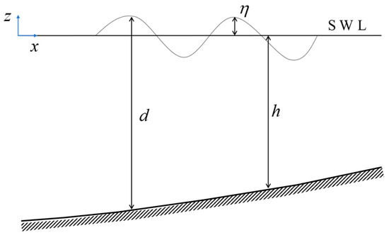
Figure 2.
The sketch of variable definitions.
To facilitate the finite-volume numerical discretization, the above Equations (1) and (2) are rewritten in the conservation form as follows:
In the above equation, is the conserved variable vector, is the flux vector and is the source term. To obtain the equilibrium between the numerical flux and the source term, the equation is rewritten as , then each vector can be defined as follows:
The specific expressions for U(q) and Sd in the above equations are shown below:
In Equation (7), f represents the coefficient of bottom friction, which is approximately in the range of 0.0001–0.01.
The details of the hybrid numerical implementation are referred to Fang et al. [43], and the main procedures are summarized for completeness. The conservative governing Equation (4) is integrated over an arbitrary control volume Ω by using the cell-centered FV method.
where Ω is the boundary of the control volume, dΓ is the arc element and nx is the outward unit vector normal to Ω. The computation domain is discretized into finite rectangular cells, and integrating the control Equation (10) in the conservation form within the finite volume and applying Green Theorem, the discrete equations can be obtained as follows:
The terms and in Equation (11) represent the numerical fluxes at the cell boundaries and , respectively, and represents the spatial numerical averages of in the cell at the moment; denotes the numerical source term.
The numerical solution of Equation (11) must begin with the calculation of the numerical fluxes at the cell interface. There are many high-resolution methods (e.g., Roe format, HLL format) available for the calculation of numerical fluxes, of which the HLL format is the most widely used. The traditional HLL format [44] not only calculates the characteristic wave velocity but also determines the Riemann solution of the characteristic wave state, which is a complicated computational process. In recent years, Toro [45] proposed the novel format of MUSTA, which not only has the characteristics of intuitive and concise expression but also does not need to solve the characteristic wave state of the Riemann solution and the characteristic wave velocity. In this model, the MUSTA format is used to solve the interface numerical fluxes, and the fourth-order accuracy interpolation method is used to reconstruct the interface left and right variables to further improve the accuracy.
The time integration of the equations is carried out using the third-order Runger-Kutta method [27] with TVD properties, and the time step is chosen using the CFL stability condition to ensure computational convergence. In the case of wave breaking, a mixed format is employed. When breaking occurs, the nonlinear terms and dispersion in Boussinesq Equations (1)–(3) are omitted and do not participate in the calculations. This results in the degradation of the equations to the fully nonlinear shallow water equations and treating the wave-breaking process as a water jump. For handling dynamic boundaries, the model adopts the effective thin-layer water body method [46]. In this paper, a very small water depth threshold is set at 0.001 m. If the water depth at a grid point exceeds this threshold, the location is classified as a water area; otherwise, it is considered as land. Simultaneously, the water depth over land is adjusted to 0.001 m, and the flow velocity is set to zero.
2.2. Wave Boundary Layer Module
In the boundary layer, the nonlinear term is usually considered to be of higher order and can therefore be ignored, resulting in a linear one-dimensional equation of the following form:
where is the flow velocity near the outer surface of the boundary layer, is the water velocity in the boundary layer, is the bottom shear stress.
Based on the Boussinesq assumption:
Equation (12) can be written as:
The boundary conditions are:
In the above equation, is the bed level, is the elevation of the outer surface of the boundary layer, and refer to the water kinematic viscosity coefficient and turbulent viscosity coefficient, respectively, and the value of υt is obtained by using the mixing-length theory:
where = 0.41 is the Kamen constant, and is the friction velocity and can be obtained from the following equation:
The driving force of the boundary layer is provided by the water–bottom velocity, which can be calculated by the following equation:
Equation (14) belongs to the classical horizontal flow and diffusion equations and can be solved using the second-order C-N format, as described in the literature [47].
2.3. Morphology Module
Numerical models of beach evolution based on dynamical processes (e.g., [17,18]) have incorporated a coastal hydrodynamic module, a boundary layer module, a sand transport module, and a topography updating module, and have become a trend in numerical modelling of beach evolution.
Hsu and Hanes [48] pointed out that the instantaneous sand transport rate under unsteady flow is closely related to the bottom shear stress in the study of two-phase laminar flow. Hsu et al. [49] also solved the sand transport rate by using the instantaneous shear stress, and in this paper, we use the Meyer-Peter–Muller sand transport rate formula strengthened by the bottom shear stress, with the expression as follows:
where is the volumetric rate of sand transport, is the rate of sand transport due to bottom shear stress and is the rate of sand transport due to the average velocity of the water outside the boundary layer. can be solved by the Meyer-Peter–Muller formula:
where can be obtained from the following equation:
In the above equations, is the Shields constant, is the Shields number at the beginning of the sand transport and and are determined empirically, with Ribberink [50] suggesting and . is the instantaneous bottom shear stress obtained from the boundary layer model.
is calculated by Bailard’s formula:
where is the time-averaged value of the bottom velocity , is the bed slope angle relative to horizontal plane, is the combined wave current friction coefficient, is the bedload transport efficiency, is the suspension transport efficiency and is the sediment fall velocity.
Sediment mass conservation equations can be used to solve the changes of beach topography under the waves.
where
In Equation (25), represents the total volumetric sand transport rate; denotes the total buoyant weight transport rate; zd is the topographic height; ρs is the density of sediment and ρ is the density of water; and ξ is the sediment porosity, which is usually taken to be 0.4 in size.
Equation (25) has strong nonlinear characteristics, which makes it difficult to solve, and topographic instability will occur due to the accumulation of time when it is solved using the ordinary differential format, which requires a higher-resolution computational format. In this paper, the Euler-WENO numerical format derived by Long [47] is used for the solution, which is suitable for calculating smooth structures containing several complex flows and different types of discontinuities.
3. Hydrodynamic Validations
3.1. Validations of Wave Boundary Layer
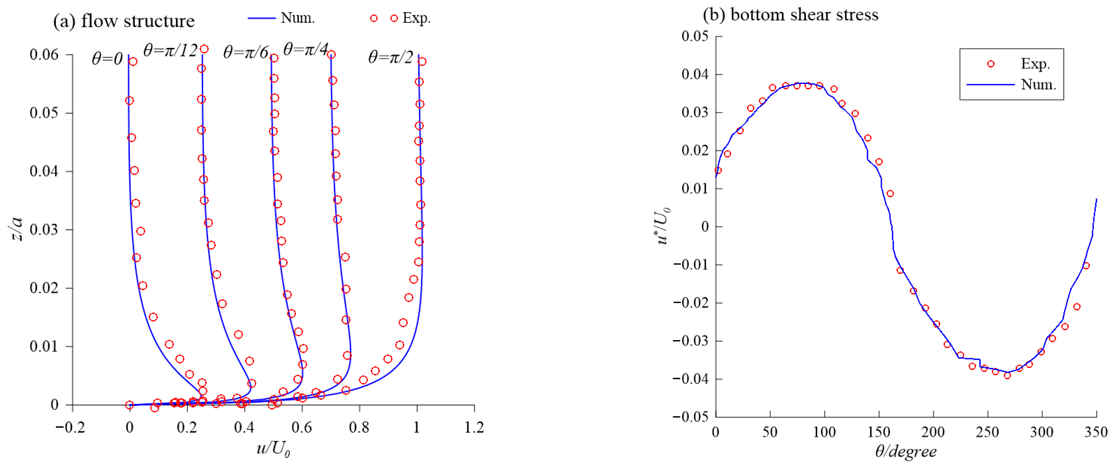
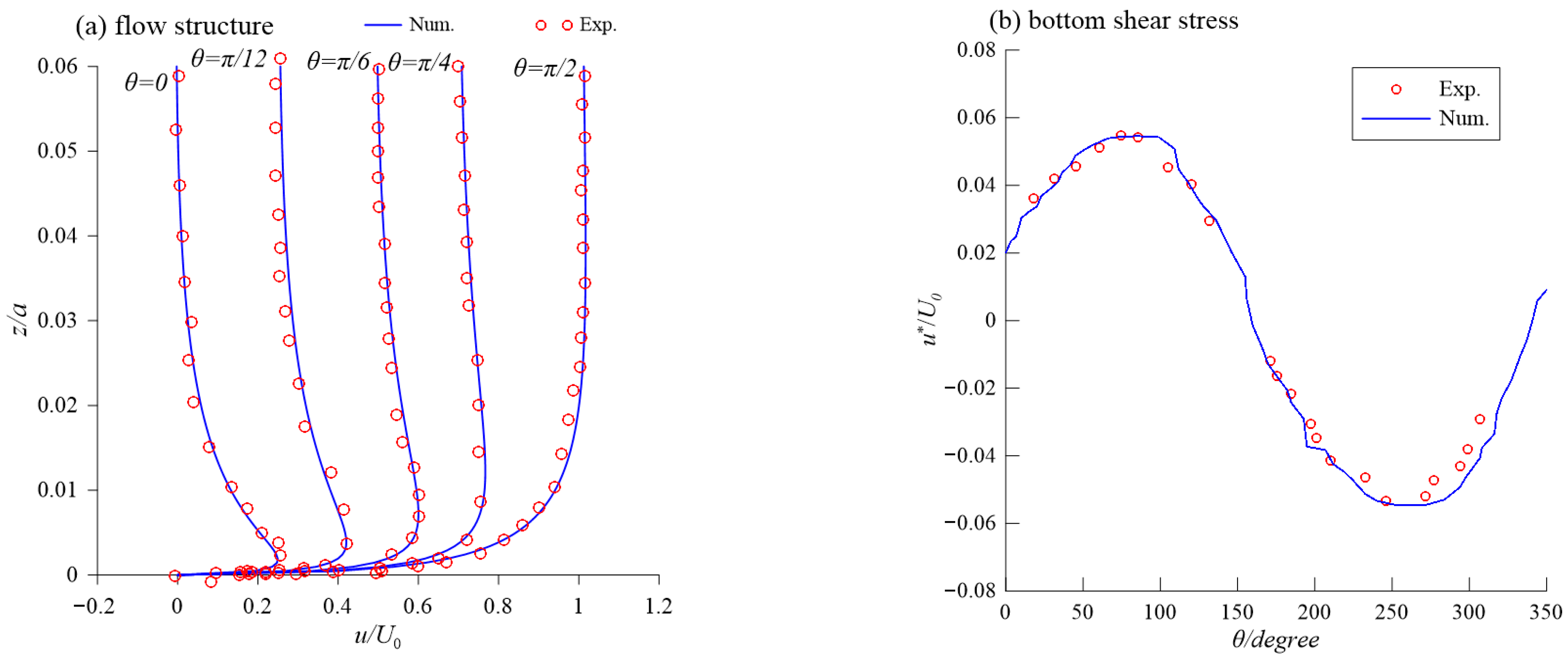
In this section, the boundary layer model is investigated under smooth and turbulent flow conditions using experiments Test 10 and Test 13 from Jensen and Fredsøe [51]. The experiments were conducted inside a U-shaped pipe, so the vertical velocity can be considered zero. The experimental area is 10 m long, 0.39 m wide and 0.28 m high, and the expression for the bottom flow velocity is:
where U0 is the amplitude of the flow velocity, and tanh is used to control the ub so that it can change smoothly. In Test 10, the amplitude of the free stream velocity is U0 = 2 m/s, the orbital excursion amplitude is a = 3.1 m, the viscosity is υ = 0.0114 cm2/s, the period of free stream oscillatory flow is T = 9.72 s and the Reynolds number is Re = 6 × 10⁶. The vertical grid size in the boundary layer is Δz = 0.0015 m, and the time step is Δt = 0.01 s. In Test 13, the parameters are unchanged and the bottom bed roughness is set to Ks = 0.84 mm.
Figure 3 shows the comparison between the experimental data and numerical results of the flow structure and the friction velocity in the boundary layer under smooth flow conditions (Test 10), and Figure 4 shows the comparison between the experimental data and numerical results under turbulent flow conditions (Test 13). The parameters in the figure are dimensionless, and the bottom shear stress is indicated by the friction velocity u* in Figure 3b and Figure 4b. The experimental data and the numerical simulation results are in good agreement, and the model is able to accurately characterize the flow velocity distribution in the boundary layer under different conditions.
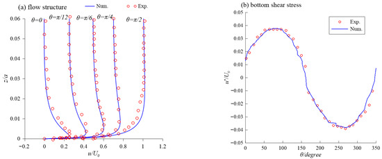
Figure 3.
Flow structure and bottom shear stress for smooth wall boundary layer in Test 10.
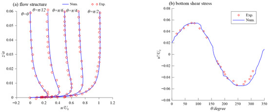
Figure 4.
Flow structure and bottom shear stress for rough wall boundary layer in Test 13.
3.2. Validations of Solitary Wave
The solitary wave is a limiting case of the cnoidal wave, and the wave surface elevation η can be represented by a first-order solution of the Boussinesq equation:
where η is the water surface elevation; H is the solitary wave height; h is the water depth; t is the time; c is the wave speed; g is the gravity acceleration.
Synolakis [52] experimentally studied the propagation of solitary waves on a uniform slope, and the experiments showed that the magnitude of the wave nonlinearity in shallow water is mainly affected by the relative wave height ε = H/h, and as the relative wave height increases, the nonlinear effects become progressively stronger, which in turn leads to a change in the waveform of the solitary waves.
The slope gradient in the Synolakis experiment is 1:19.85, and the experiment result shows that the solitary wave will break up when ε > 0.029. Firstly, the non-breaking condition of the solitary wave is examined, the wave height is H = 0.006 m, the still water depth is h = 0.3106 m and the relative wave height is ε = 0.019. In the numerical calculation, the length of the computational domain is 60 m, the foot of the slope is 19.85 m away from the left boundary of the model and the slope is 1:19.85. The spatial step length is Δx = 0.2 m, the time step length is Δt = 0.1 s and the total simulated time is 50 s. An internal wave generation method is used in the numerical model, and the wavemaker is located 5.17 m from the left end of the model, the right end of the model is the solid boundary, and a sponge layer with a length of 4.0 m is placed at the left end to dissipate the waves.
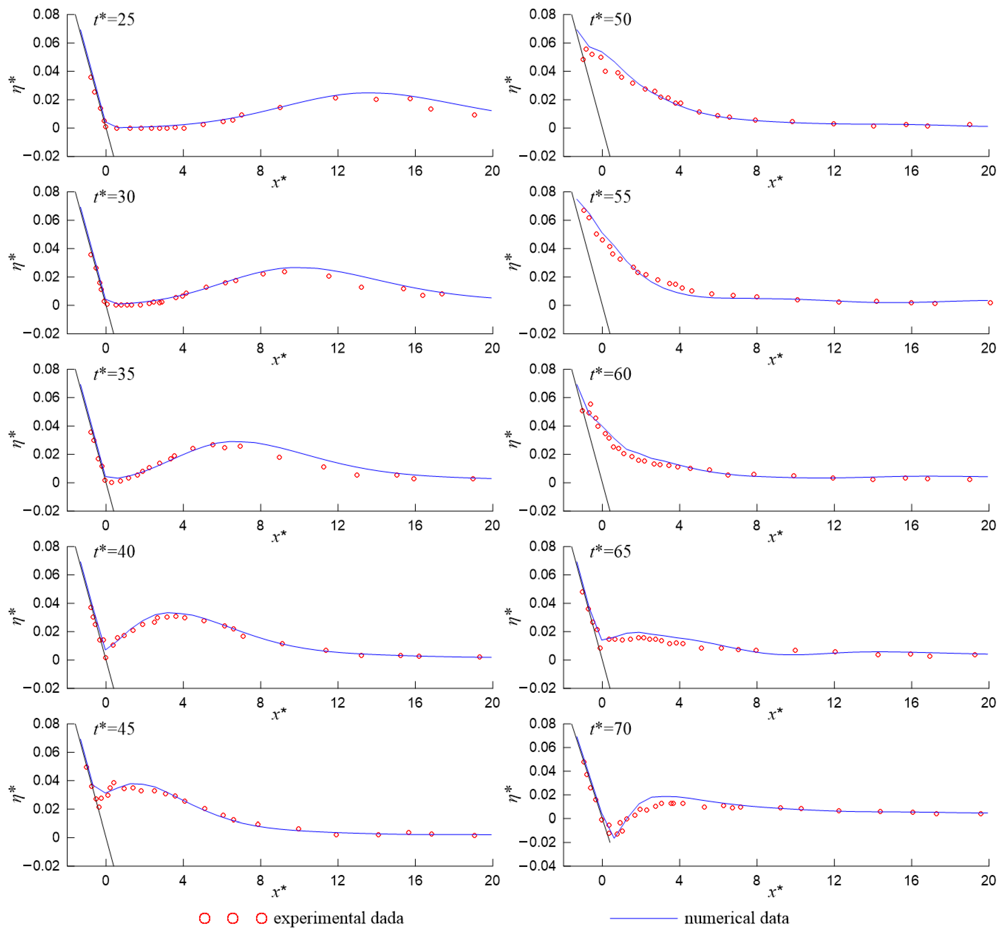
The comparison of the calculated results with the measured data is shown in Figure 5, where is the non-dimensional length, is the non-dimensional water surface elevation, and is the non-dimensional time. As can be seen from the figure, the numerical simulation results are in good agreement with the experimental results, and the numerical results are slightly larger than the experimental results because the model does not consider the bottom friction in the calculation.
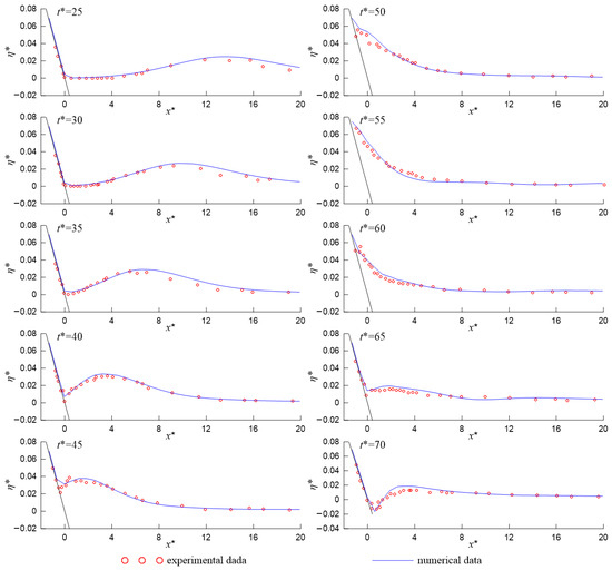
Figure 5.
Comparisons of wave evaluations between numerical results and experimental data at different moments of the non-breaking condition.
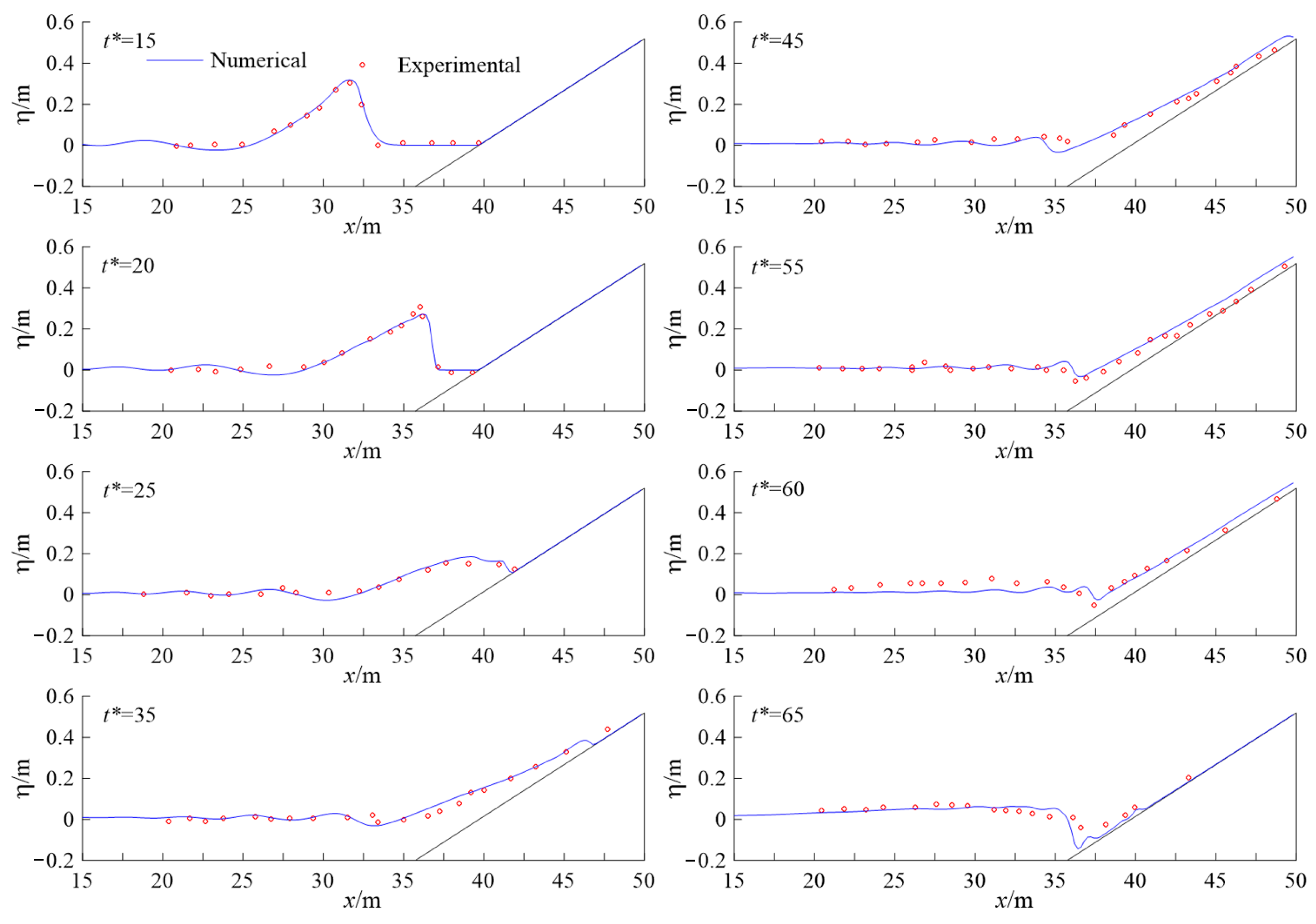
Secondly, the breaking condition is calculated, the solitary wave will break up at ε = 0.3 on a slope of 1:19.85; at this time, the wave height is H = 0.3 m, the still water depth is h = 1.0 m, the length of the computational domain is 60 m, the foot of the slope is 19.85 m away from the left boundary of the model. Other settings of the numerical model are consistent with the non-breaking condition. The comparison between the model and the experimental data is shown in Figure 6, and the numerical simulation results are in good agreement with the experimental data both in terms of the waveforms of the solitary waves and the changes in the wave heights.
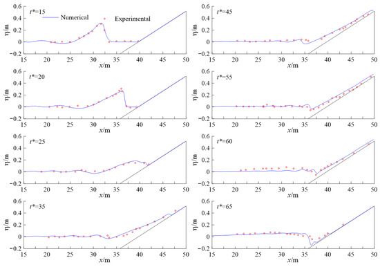
Figure 6.
Comparisons of wave evaluations between numerical results and experimental data at different moments of the breaking condition.
From the simulation process, it can be seen that when the solitary wave propagates in the region of constant water depth, the wave shape remains essentially unchanged. On the slope, as the water depth gradually decreases, the solitary wave is affected by the shallow water effect, the amplitude of the water point in front of the wave crest decreases and the wave height also decreases, as can be seen from the figure at the moment of t* = 20, the whole solitary wave is in a right-leaning state. As the wave crest moves towards the slope, the whole wave starts to climb up the slope. At the moment of t* = 25 in the figure, there is a “trough” in the middle of the wave surface, which is caused by the speed of the water point behind the wave crest being less than the speed of the crest point. As the solitary wave climbs up the slope, the wave breaks, then jumps forward, and finally reaches its maximum height. At this point, the kinetic energy of the water particle is completely converted into potential energy. After that, the body of water is affected by gravity, and the water particle falls back and slides down the slope, leaving a thin layer of water on the slope, as shown in the figure at the moment t* = 65.
Through the above simulation of non-breaking solitary waves and breaking solitary waves propagating on a uniform slope, it can be found that the numerical simulation results are in good agreement with the experimental results of Synolakis [52], which verifies that the model has a good ability to capture the dry and wet dynamic boundaries and to deal with the breaking case. More simulation experiments of hydrodynamic processes have been given by Fang et al. [43]. The comparison and discussion between other methods show that the MUSTA scheme has almost identical numerical accuracy but requires slightly less computation time and is much easier to code.
4. Morphology Validations
4.1. Sandbar Evolution under Bragg Resonance
The interaction between sandbars and waves has been studied, and it has been found that waves erode the crests of the sandbars, while the troughs are filled with sediment, causing sandbars on the inshore side to disappear and new sandbars to form on the flat bed offshore. If the wave length of the sandbank is similar to that of the waves, the deformation of the sandbank is mainly influenced by local standing waves and gravity.
In this section, the previously developed wave model is used to simulate the wave propagation, the bottom shear stress is calculated by the boundary layer model and the sand transport rate is calculated using the bedload sediment transport equation of Meyer-Peter and Muller [41]. In the numerical model, several sandbars with sinusoidal regular shape variations are given on a flat bed. Initially, the sandbars are placed in an area of 400 m < x < 700 m, while the rest of the area is flat. The wavelength of the sandbar is half of the wavelength of the incident wave, the depth of the still water is h = 7 m, the wave is incident at x = 160 m with amplitude A0 = 0.5 m and period T = 8.0 s. A sponge layer is placed at x = 860 m to absorb the wave. The shape amplitude of the underwater sandbar is given by the following equation:
Based on Equation (29), the amplitude of the sandbar can be calculated as Ab = 0.64 m. In the numerical calculations, the time step is ∆t = 0.05 s, the spatial step is ∆x = 0.2 m, the sediment density is ρs = 2650 kg/m3, the sediment grain size is d = 0.4 mm, the porosity is ξ = 0.4 and the coefficients are A = 11.0 and b = 1.65.
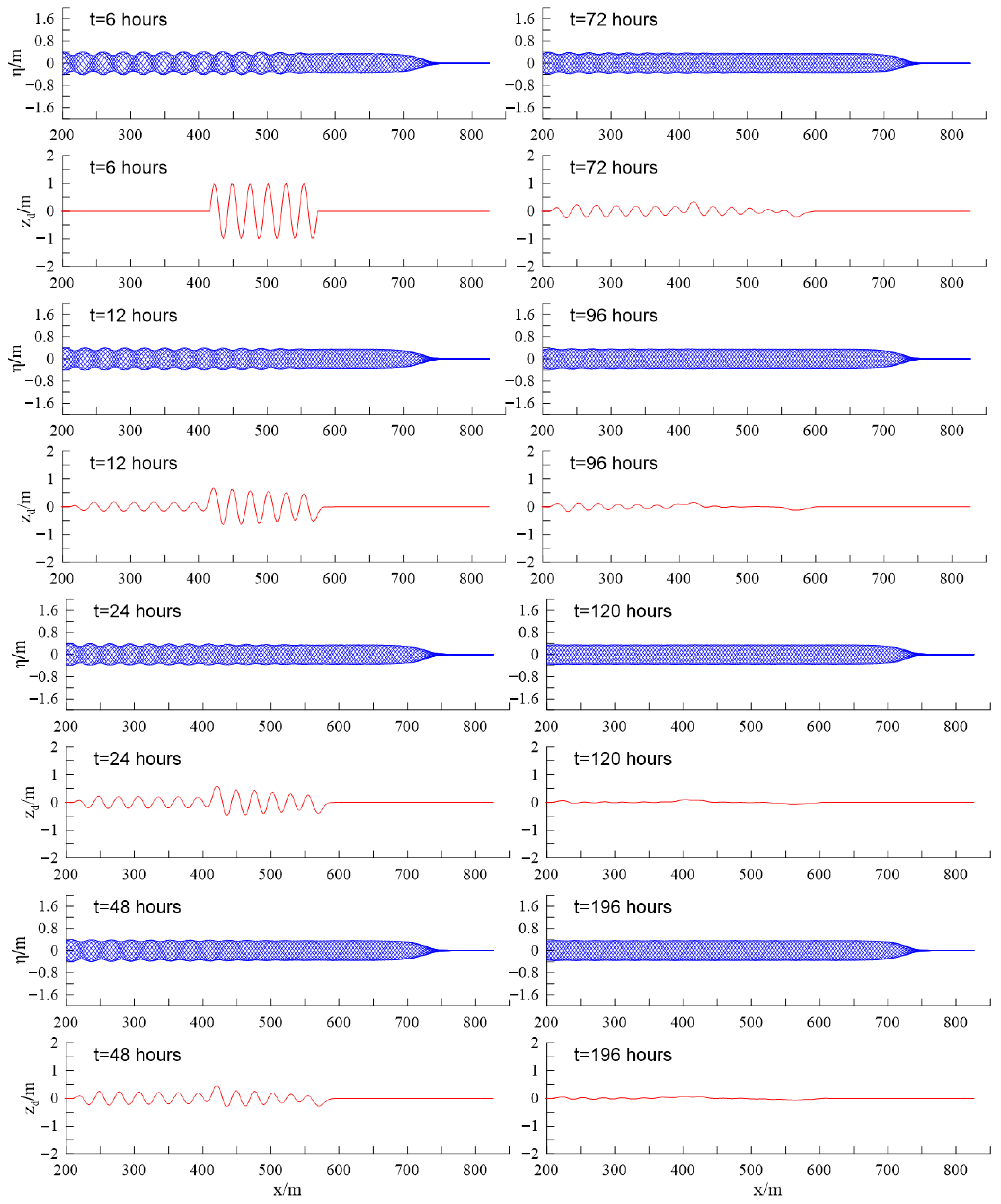
Figure 7 shows the evolution of wave surface and underwater sandbars over time. As the crest of each sandbar is π/4 phase ahead of the wave node and lags π/4 phase behind the next wave loop, when the wave passes over the sandbar, the sandbar on the shore side is affected by Bragg’s reflection, the wave crest is eroded and thus reduced, while the trough of the sandbar is silted up and gradually filled in; at the same time, a new sandbar is created on the offshore side, and the increase rate of the new sandbar is faster in the beginning, such as the moment of t =12 h.
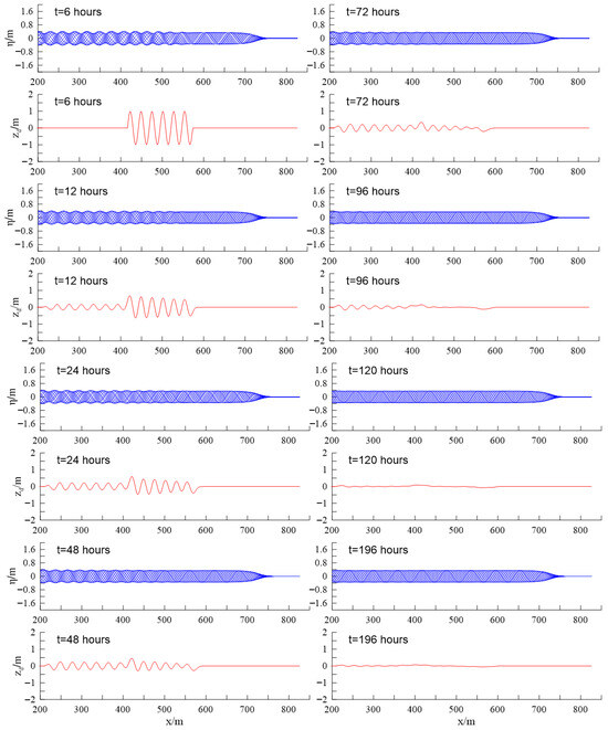
Figure 7.
Wave envelopes and bed elevations at different moments.
In the following moments, the initial sandbars gradually shrink, and the growth rate of new sandbars gradually slows down. As time passes, at t = 196 h, the preexisting sandbars slowly flatten under the influence of the Bragg reflection, while the newly formed sandbars on the offshore side are also attenuated by the weakened Bragg reflection, and eventually all these sandbars will disappear. The numerical simulation results in Figure 7 show the process of the original sandbars decreasing, new sandbars emerging and finally all sandbars disappearing, resulting in a flattened terrain.
4.2. Sandbar Generation under Solitary Waves
Young et al. [36] carried out an experimental study of beach deformation under a solitary wave height of H = 0.6 m. In the experiment, the slope front was a flat-bottomed terrain, and the still water depth in front of the slope was h = 1.0 m. The experimental terrain was a 1:15 gradient slope with a slightly undulating surface similar to an S-shaped distribution.
In the experiment, the foot of the slope is located at x = 12 m, the wave maker is located at x = 10 m and the waves begin to generate and propagate towards the shore at the moment t = 0 s. In the experiment, the wave height gauges were placed at four positions, x = 23 m, 25 m, 27 m and 29 m, to measure the change in the water surface. The velocity instruments were placed at x = 23 m, 28 m and 29 m to measure the water velocity. At the same time, Young et al. [36] counted the topographic changes of the shoreline after 3, 6 and 9 groups of solitary waves, and waiting 15 min after the end of the previous group of waves in order to ensure that the water surface and the topography were in a stable state each time.
In the numerical model as shown in Figure 8, the foot of the slope is located at x = 140 m, the wavemaker is located at x = 40 m and a 20 m long sponge layer is installed on the left to absorb the waves. The numerical model has time step ∆t = 0.01 s and space step ∆x = 0.2 m, and the terrain is updated every 0.01 s in the model calculation. The water density is ρ = 1000 kg/m3, the sediment grain size is D50 = 0.4 mm, the sediment density is ρs = 2650 kg/m3, the sediment settling speed is = 0.02 m/s, the sediment porosity is ξ = 0.4, the suspending mass efficiency coefficient is εs = 0.01, the bedload mass efficiency coefficient is εb = 0.135, the sediment internal friction angle is = 32° and the friction coefficient is = 0.02. In the experiment, the locations of four wave height gauges in the numerical model correspond to x = 151 m, 153 m, 155 m and 157 m, respectively, and the locations of the velocity instruments correspond to x = 151 m, 156 m and 157 m, respectively.
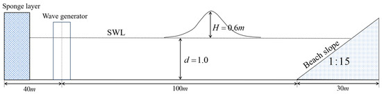
Figure 8.
The illustrative diagram of the numerical water tank.
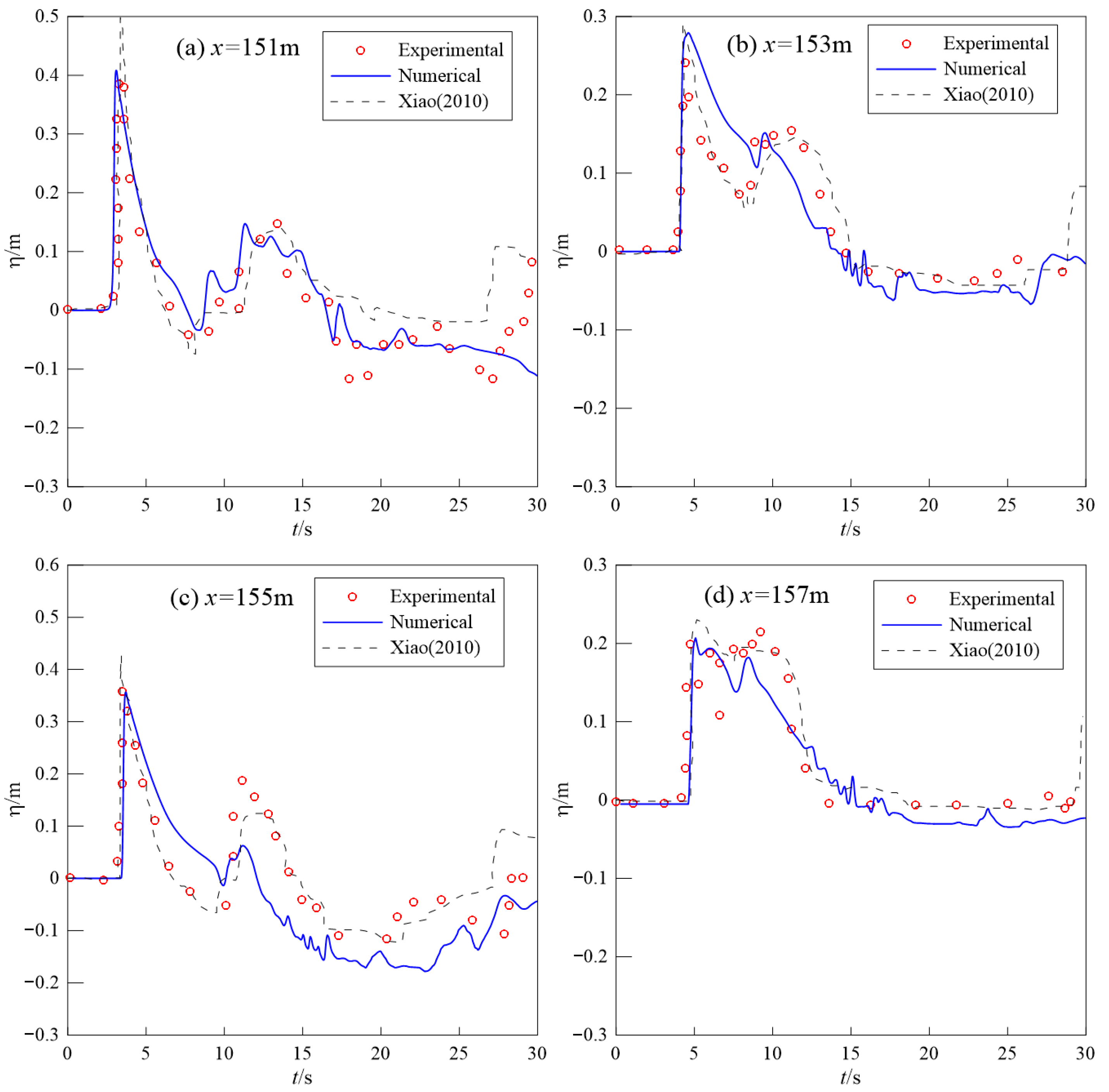
Figure 9 shows the evolution of the water surface over time at four positions: x = 151 m, 153 m, 155 m, 157 m. As can be seen in the figure, the water surface changes from horizontal to almost vertical at t = 2.5 s, and the wave front becomes steeper and the waveform tilts forward due to the effect of the shallow water. There are two water surface peaks at x = 151 m, 153 m and 155 m caused by two processes: the wave rising along the shore and the wave falling back after reaching the highest point. The numerical results of the two peaks are in good agreement with the experimental data, and only the second peak at x = 155 m is underpredicted, which may be due to the stronger reflected wave action at this location. Overall, the numerical model can accurately simulate the whole process of wave propagation, including deformation, breaking, collapse and the interaction between waves.
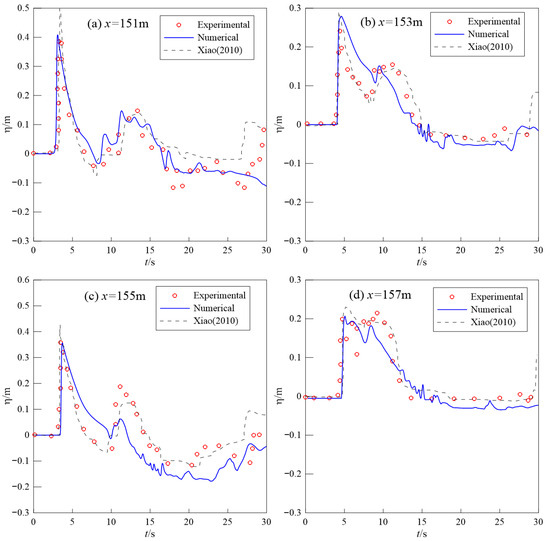
Figure 9.
Time series of water surface elevation at four locations [37].
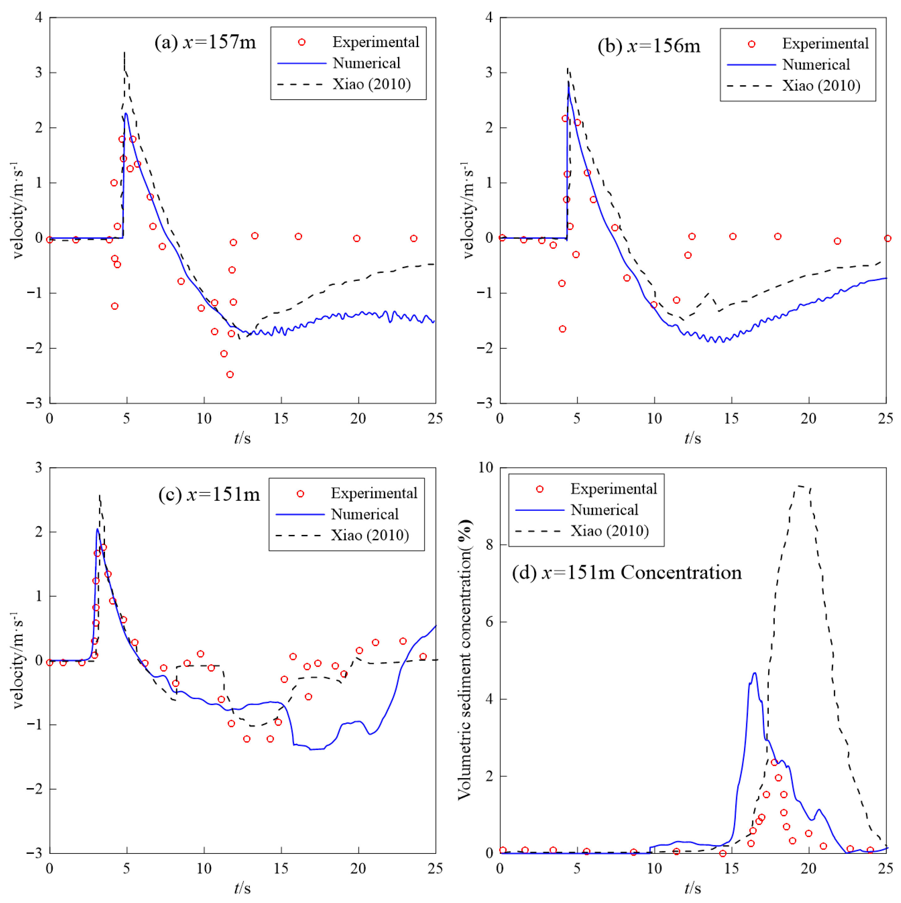
Figure 10 shows the variation of flow velocity at three locations, x = 151 m, 156 m and 157 m, and the volumetric sand concentration at x = 151 m, respectively. Experimental data and numerical results from Xiao et al. [37] are used in the figure for comparison with the results of this paper. The experimental values at x = 156 m and 157 m in the figure are slightly unstable at the moment t = 5 s, which is due to the fact that the initial moment of the velocity instruments at these positions is relatively dry, resulting in the experimental data not yet being stable. After t = 5 s, the velocity instruments have been stabilized, and the experimental data are more accurate, and the numerical values are basically in agreement with the experimental data.
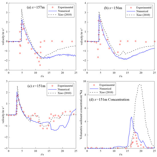
Figure 10.
Time series of velocities and volumetric sediment concentration at three locations [37].
The figure also shows that the model accurately predicts the peak flow velocity at three locations. After the time t = 12 s, the numerical simulation results have a large deviation from the experimental data, mainly due to the fallback of the wave, resulting in the velocity instruments at the locations x = 156 m and 157 m being exposed to the water surface again; the flow velocity data could not be collected and become zero.
Figure 10d shows the variation of sand concentration in the water at x = 151 m. Comparing the experimental data and the model results of Xiao et al. [37], the peak time of sand concentration calculated by the model in this paper is advanced, and the peak value is slightly larger than the experimental data. In contrast, the peak time calculated by Xiao et al. [37] is relatively delayed and the peak sand content is much larger than the measured value. The reasons for the differences between the numerical results and the measured data may be as follows: firstly, the model calculations of flow velocity and sand concentration are based on the simulation of water depth averaging, whereas the instrumental observation is for a specific point; secondly, the sand content of the numerical model includes both suspended sediment and bedload sediment, whereas the experimental instrumentation mainly measures the suspended component of the water. Overall, the calculation results of the shoreline evolution model in this paper are more accurate.
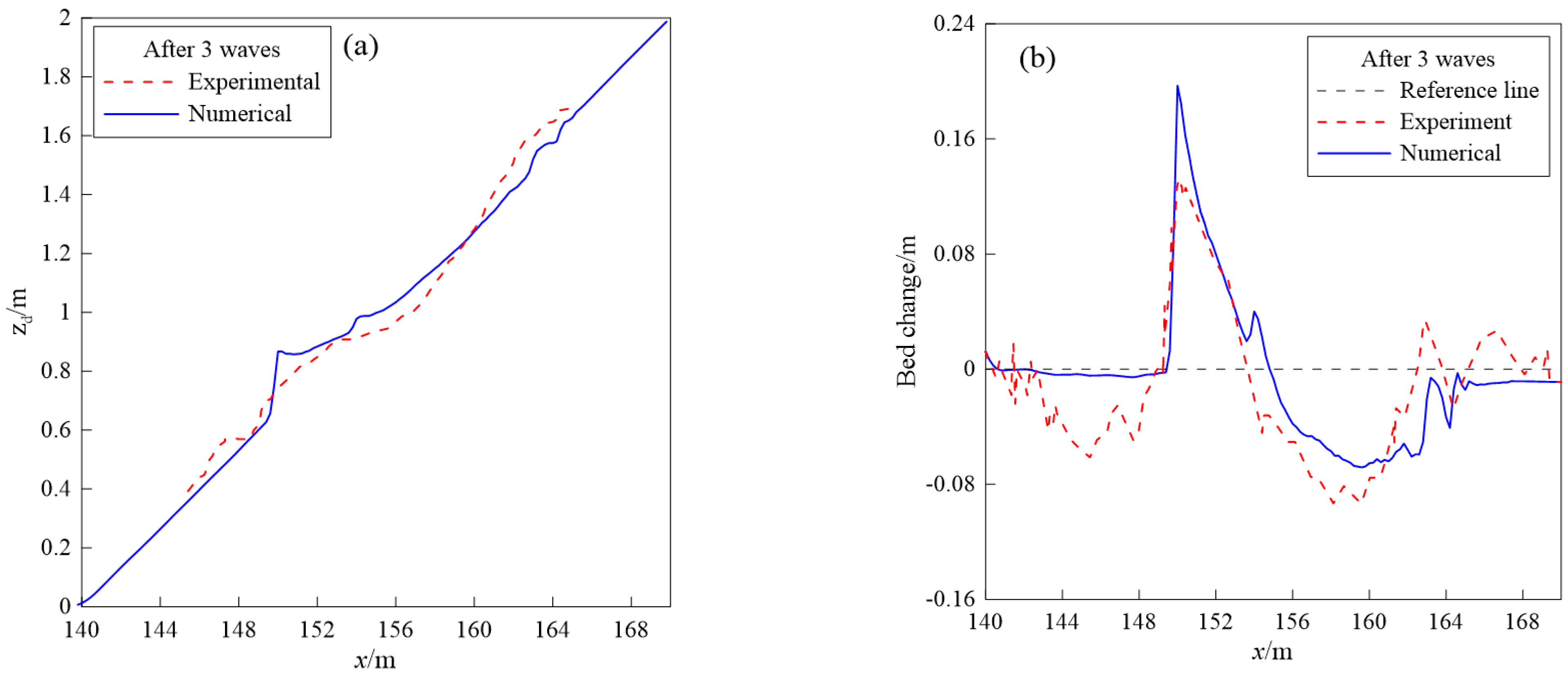
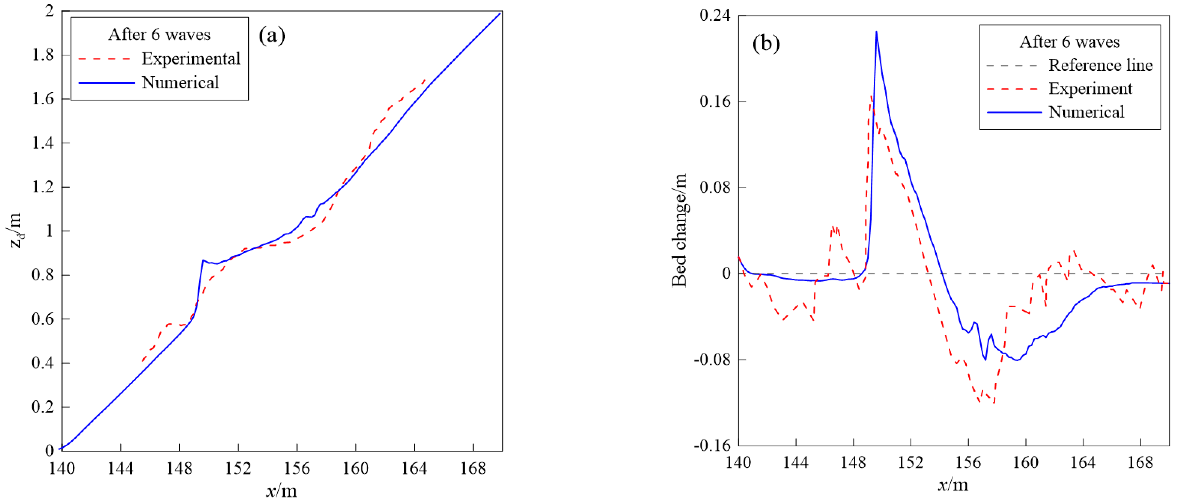
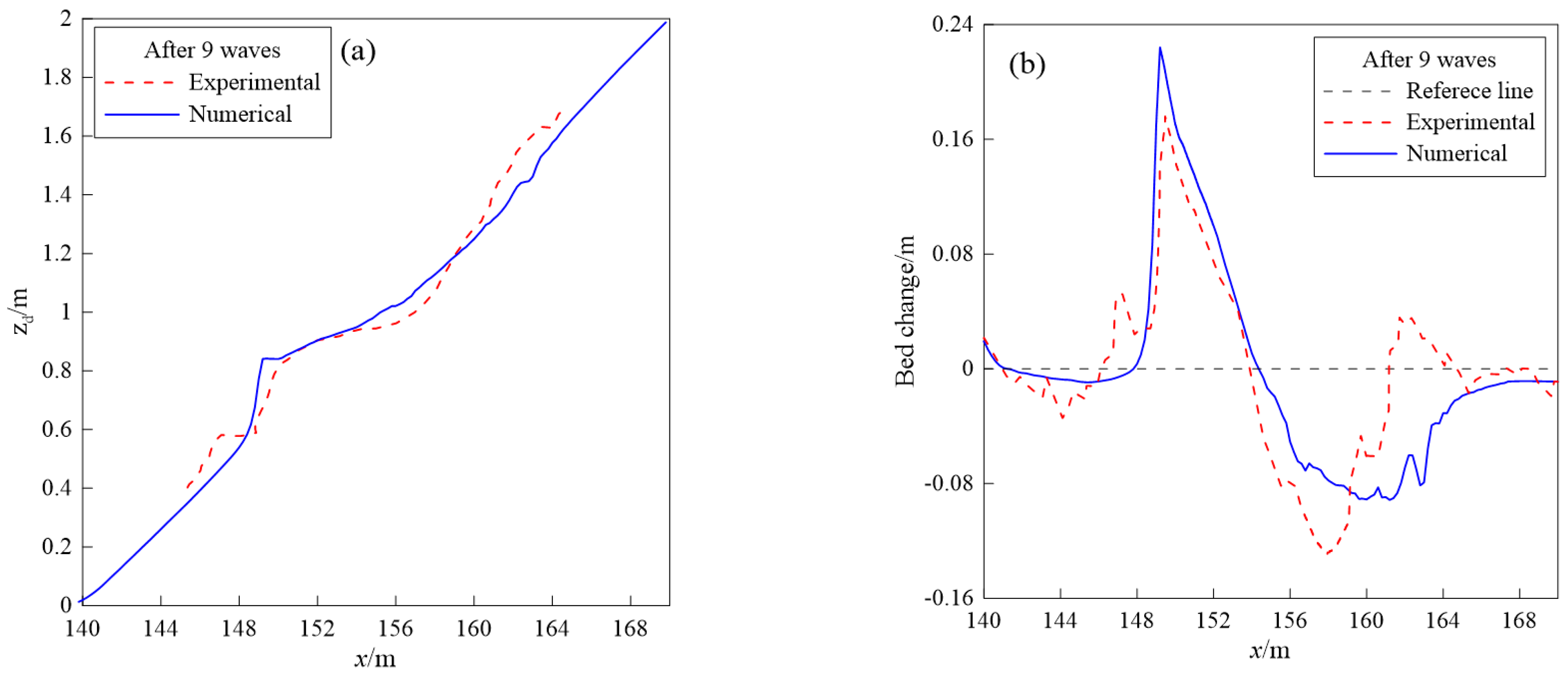
Figure 11, Figure 12 and Figure 13 show the topographic changes of the shoreline after the action of 3, 6 and 9 sets of wave conditions, respectively. It can be seen from the figures that deposition occurs on the shoreline surface in the region of 150 m < x < 153 m, then sandbars appear and the topographic change in the shoreline reaches its maximum value at the position of x = 152 m. This area is near the wave-breaking point, the phenomenon of water jump will occur after the wave climbs, and when the wave falls back, the water jump cycle will occur. This leads to a decrease in the flow speed in the area and a decrease in sediment-carrying capacity, resulting in the fall of sediment silt, so in the water jump cycle will appear a large amount of sediment accumulation and thus the formation of sandbars.
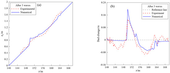
Figure 11.
Profile and topographic changes due to 3 groups wave action. (a) Profile change, (b) Topographic change.
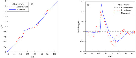
Figure 12.
Profile and topographic changes due to 6 groups wave action. (a) Profile change, (b) Topographic change.
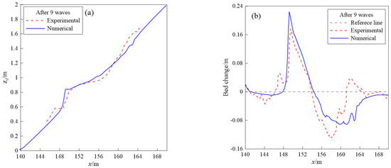
Figure 13.
Profile and topographic changes due to 9 groups wave action. (a) Profile change, (b) Topographic change.
From the figure, we can also see that the changes in length and height of the topography after each wave group are similar, which is about 2–4 cm. In the region of 153 m < x < 157 m, the surface of the beach is eroded and pits appear. This is because the speed of the falling current is larger in this region, and the water depth is shallower, which results in an increase in the shear stress at the bottom of the water, and promoting the activation of sediments and the formation of erosion. The increase in beach deposit and the decrease in erosion are approximately equal in value, in accordance with the law of conservation of matter.
4.3. Sandbar Generation and Migration under Regular Waves
Experiments R3 and R4 on sandbar formation under regular waves completed by Yin [53] were selected to validate the model. The experimental flume was 56 m long, 0.7 m wide and 1.0 m high, with a pusher-plate wavemaker at the left of the flume, and a sandy beach model at the right of the flume, and the still water depth is h = 0.45 m on the flat bottom. The experimental parameters are given in Table 1, and the experiments were carried out to study the evolution of the beach profile at two slopes, 1:10 and 1:20, respectively.

Table 1.
Parameters for the incident wave.
In the numerical simulation, the foot of the coastal slope is located at x = 20 m, the wavemaker is located at x = 10 m and a sponge layer is placed to the left of the computational domain to minimize wave reflection. The topography was updated in the computation every 12 min, and the computation time was 1 h for both conditions. The sediment particle size is D = 0.4 mm, the sediment porosity is ξ = 0.4, the sediment density is ρs = 2650 kg/m3, the water density is ρ = 1000 kg/m3, the bedload mass efficiency coefficient is εb = 0.135, the suspending mass efficiency coefficient is εs = 0.01, the sediment settling speed is = 0.03 m/s, the sediment internal friction angle is = 32° and the friction coefficient is = 0.05.
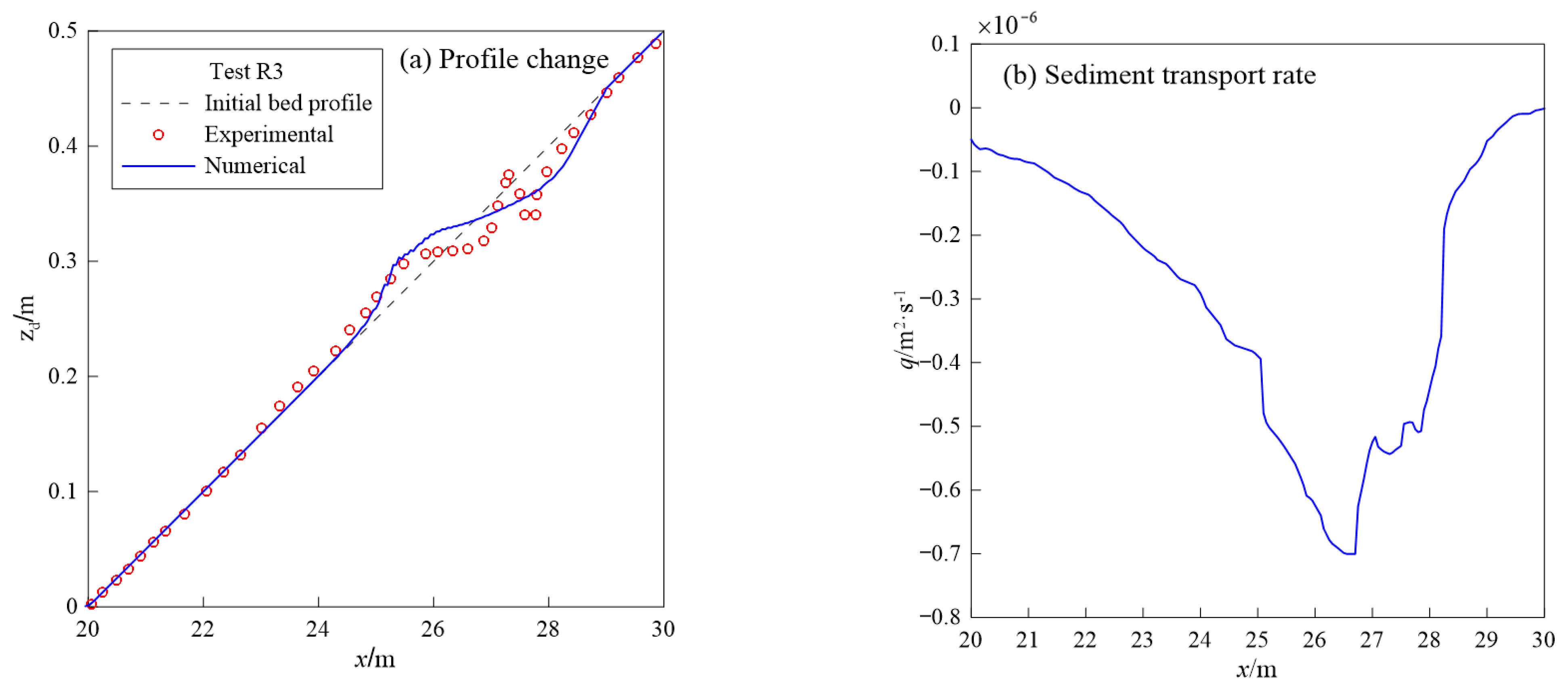
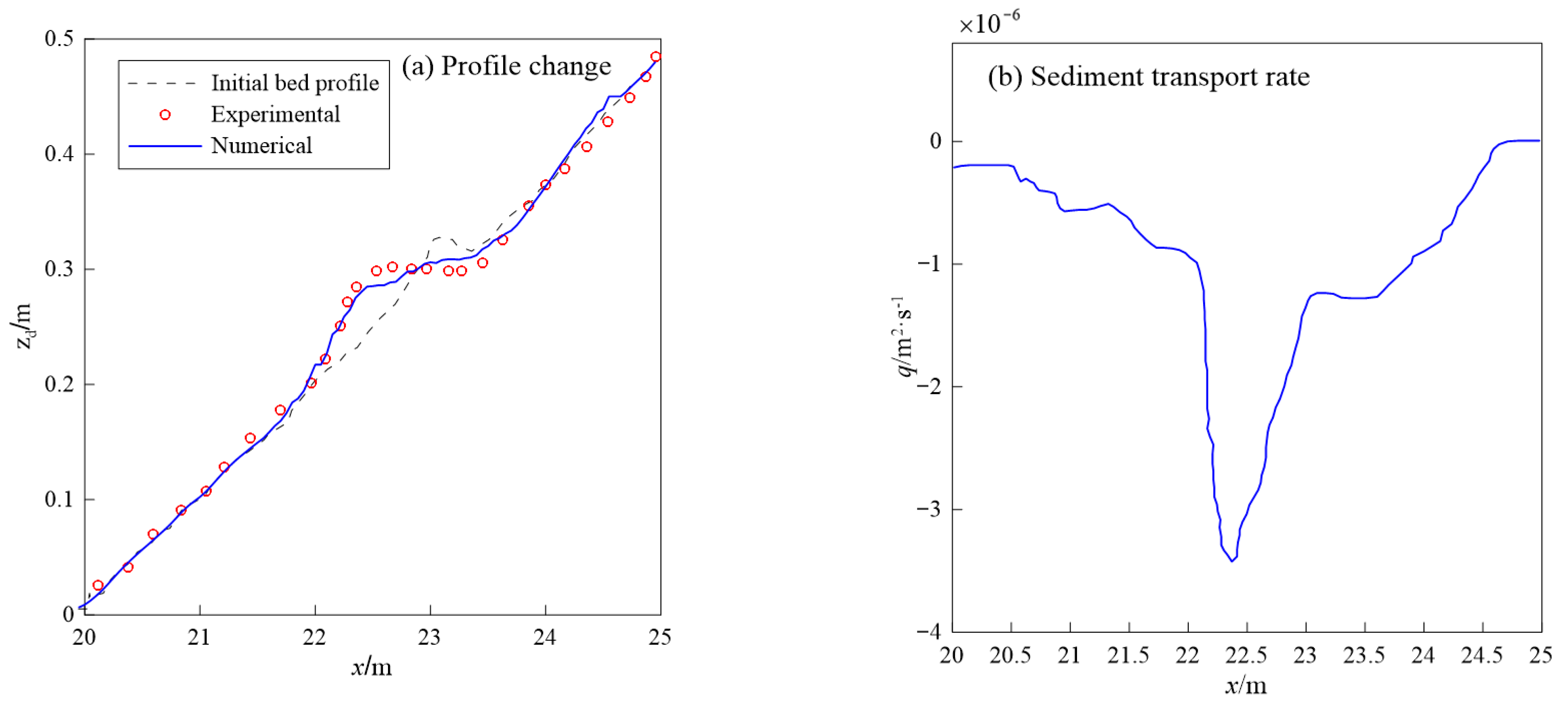
Figure 14a shows the comparison between the simulated values and the experimental data for the change in beach profile under wave condition R3. It can be seen that the experimental data and the numerical results are in better agreement, and the simulated values accurately simulate the location of sandbars and the change in beach profile. Figure 14b shows the distribution of the sand transport rate calculated by the model, which is positive for the onshore sand transport and negative for the offshore sand transport. It can be seen in the figure that the offshore sand transport rate is dominated in the nearshore, and the sand transport rate reaches a maximum at the junction of the erosion and siltation, which is basically consistent with the phenomenon of siltation occurring on the offshore side to form a sandbar, and erosion occurring on the onshore side to form a scour pit.
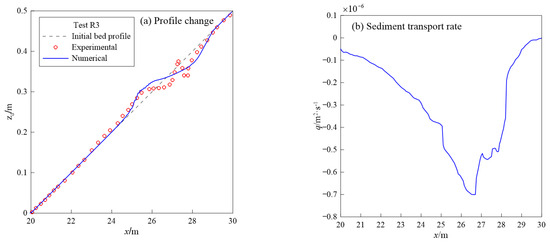
Figure 14.
Change in bed profile and sediment transport rate under Test R3 for 1 h.
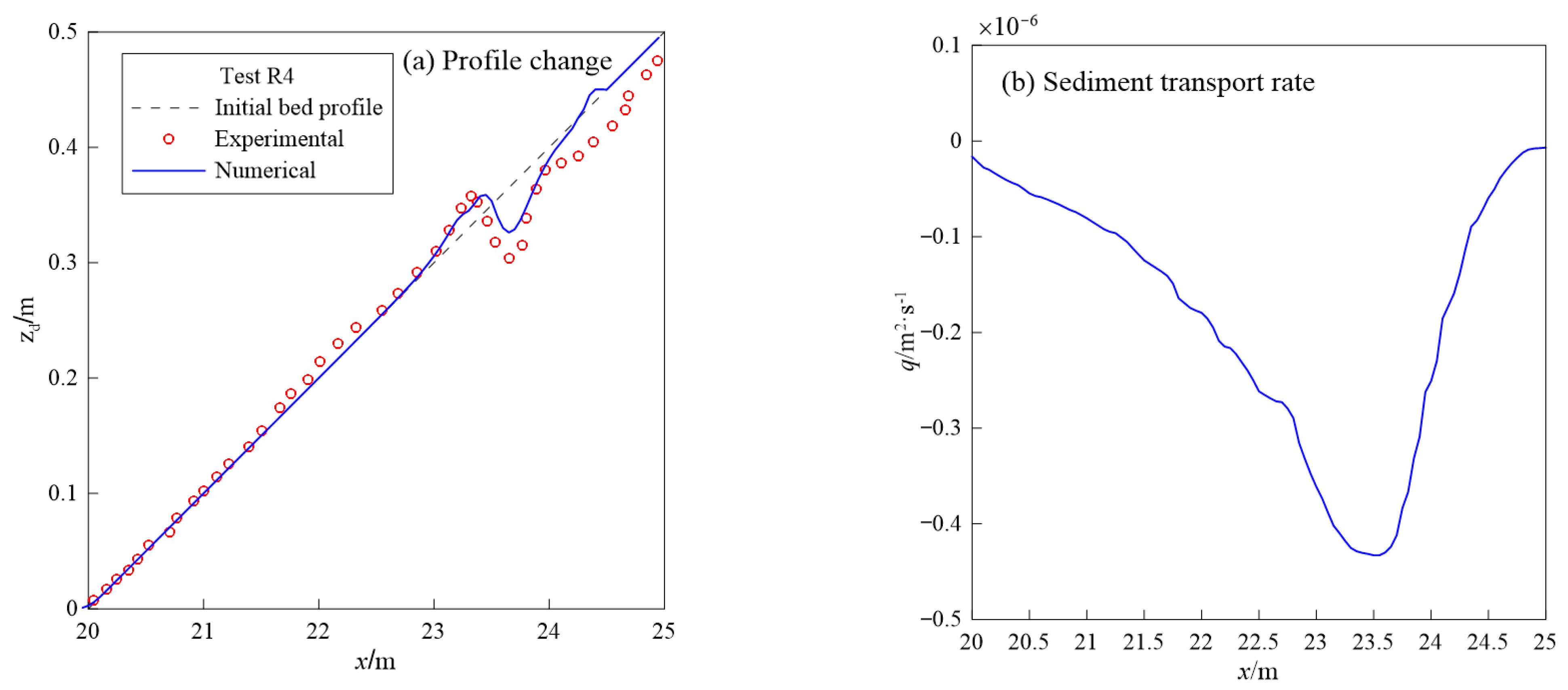
The comparisons for the wave condition Test R4 are shown in Figure 15a. The numerical model accurately simulates the location of the sand bars and the changes in topography, and the distribution of the sand transport rate is shown in Figure 15b. The wave action produces strong water turbulence, which will lead to an increase in shear stress at the water bottom and promotes sediment activation; at the same time, the backward current after the wave climbs will produce strong sediment transport, making the coast of the region form a scour pit. When the wave breaks on the beach, the body of water undergoes strong turbulence, and the backflow of wave forms a sand-carrying current in the offshore direction. After the sand-carrying current crosses the wave-breaking point, the sand-carrying capacity of the current rapidly decreases, the offshore sediment transport will slowly stop due to the block of the onshore current and eventually sediment will be deposited near the breaking point, forming a sandbar.
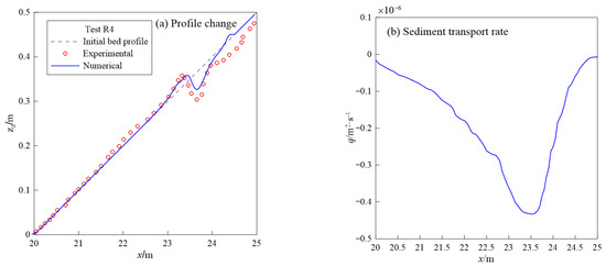
Figure 15.
Change in bed profile and sediment transport rate under Test R4 for 1 h.
Natural coastlines usually have sandbars, which make waves break away from the shore and reduce the destructive effects of waves on the coast. The position of the sandbank on the coast is not fixed and sometimes moves offshore due to wave action. Based on the numerical model, the movement of the sandbar was investigated with an incident wave height of H = 16 cm, keeping the other conditions the same as in test R4 and changing the terrain to a slope with an approximate slope of 1:10 with a sandbar on it.
The results of the evolution of the sandbar profile after 45 min under regular waves were analyzed, and the comparison of the computed results with the experimental data is shown in Figure 16a. It can be seen from the figure that the offshore motion of the sandbar occurs under the action of the waves, and the position of the sandbar calculated by the model is almost identical to the measured data in the experiment. Figure 16b shows the distribution of sand transport rates, which are negative near the sandbars under the wave action, resulting in offshore movement of nearshore sediment, and the rate of sand transport varies with the topography and reaches a maximum at the location of the highest point of the sandbars. Erosion occurs on the onshore side of the sandbar under wave action, while siltation occurs on the offshore side, and over time the shoreline profile then shows offshore movement of the sandbar.
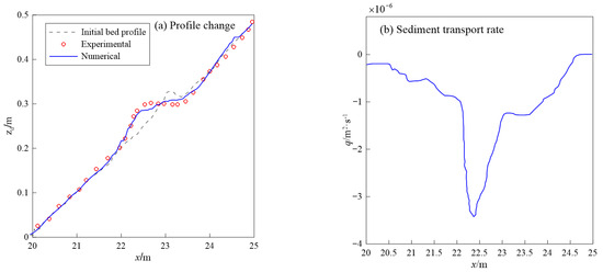
Figure 16.
Beach profile change and sediment transport rate under regular wave action.
Through the above examples, the model accurately simulates the deformation of the shoreline under the action of solitary and regular waves, and the numerical results are in good agreement with the experimental data, which proves that the numerical model of shoreline evolution established in this paper can better simulate the formation and movement process of the coastal sandbar under the different waves.
5. Conclusions
In this paper, the numerical wave model is solved based on the hybrid format, and after coupling the boundary layer model, the sand transport model and the terrain updating model, a numerical model of the shoreline profile evolution based on the dynamical process is formed, which is validated by several numerical experiments, and the following conclusions are obtained:
Compared with the traditional Boussinesq model based on the finite-difference method, a new Boussinesq-type wave model is developed based on a hybrid format of the finite-difference method (FDM) and the finite-volume method (FVM) and adopts the MUSTA format to approximate the numerical fluxes at the interface, which has a greater advantage in dealing with the case of unstable intermittent currents with better nonlinear performance. The model can accurately capture the dry and wet boundaries and can better deal with the wave-breaking problem. Through some numerical experiments, it is verified that the model has a high accuracy in the calculation of the wave boundary layer and the solitary wave, which is fully capable of simulating the wave propagation in the rapidly changing terrain.
The validity of the coupled wave model, sand transport model and terrain updating model is verified by the example of the sandbar evolution under Bragg resonance. The simulation shows that after the wave passes over the sandbar, the wave crest of the sandbar on the onshore side is eroded by the influence of the Bragg reflection and thus decreases, and a new sandbar is formed on the offshore side; and with the weakening of the Bragg reflection effect, the new sandbar will fully disappear. The numerical simulation can well reproduce the interaction between the sandbar and the wave.
Through the simulation of the beach deformation under the solitary and regular waves, it is found that during the wave climbing process, the turbulence of the water body will carry a large amount of sediment into the water body, and after the wave climbs to the highest point, the water velocity tends to be zero, resulting in the siltation of the sediment. While the water is falling back, the water bottom has a larger shear stress, which promotes the sediment activation, transport and erosion formation; near the breaking point, the water jump usually occurs, when the falling sand-carrying current is embedded to the bottom of the water jump, the sand-carrying capacity decreases, resulting in siltation of the sediment, so near the area of the breaking point, a large amount of sediment accumulation will occur, resulting in the formation of sandbars.
The comparison between numerical and experimental results shows that the numerical model of shoreline profile evolution based on dynamical process established in this paper can fully consider the interaction process between waves and nearshore topography and can accurately quantify the shoreline profile change and describe the details of the formation and movement of nearshore sandbars. The computational capability of the three-dimensional numerical model in the shoreward sediment movement should be further optimized.
Author Contributions
Conceptualization, K.F.; Methodology, P.W. and Z.L.; Software, P.W., K.F., J.S. and L.Z.; Validation, P.W., Z.L., J.S. and L.Z.; Formal analysis, P.W., K.F. and Z.L.; Data curation, J.S. and L.Z.; Writing—original draft, P.W., K.F., Z.L. and J.S.; Writing—review & editing, P.W. and Z.L.; Visualization, P.W., J.S. and L.Z.; Supervision, K.F.; Project administration, K.F. All authors have read and agreed to the published version of the manuscript.
Funding
This research was funded by the National Key Research and Development Program of China (2022YFC3106101), and the National Natural Science Foundation of China (52071057, 52171247), and Open Research Project of Hebei Marine Ecological Restoration and Smart Ocean Monitoring Engineering Research Center (HBMESO2316).
Data Availability Statement
The data that support the findings of this study are available from the corresponding author upon reasonable request.
Conflicts of Interest
The authors declare no conflict of interest.
References
- Fredsøe, J.; Andersen, O.H.; Silberg, S. Distribution of suspended sediment in large waves. J. Waterw. Port Coast. Ocean Eng. 1985, 111, 1041–1059. [Google Scholar] [CrossRef]
- Deigaard, R.; Fredsoe, J.; Hedegaard, I.B. Suspended sediment in the surf zone. J. Waterw. Port Coast. Ocean Eng. 1986, 112, 115–128. [Google Scholar] [CrossRef]
- Shibayama, T.; Nistor, I. Modelling of time-dependent sand transport at the bottom boundary layer in the surf zone. Coast. Eng. 1998, 40, 241. [Google Scholar] [CrossRef]
- Nielsen, P. Coastal Bottom Boundary Layers and Sediment Transport; World Scientific: Singapore, 1992. [Google Scholar]
- Kubo, H.; Sunamura, T. Large-scale turbulence to facilitate sediment motion under spilling breakers. In Proceedings of the Fourth Conference on Coastal Dynamics, Lund, Sweden, 11–15 June 2001; pp. 212–221. [Google Scholar]
- Ting, F.C.K. Large-scale turbulence under a solitary wave. Coast. Eng. 2006, 53, 441–462. [Google Scholar] [CrossRef]
- Ting, F.C.K. Large-scale turbulence under a solitary wave. Part 2: Forms and evolution of coherent structures. Coast. Eng. 2008, 55, 522–536. [Google Scholar] [CrossRef]
- Sun, J.W.; Fang, K.Z.; Liu, Z.B.; Fan, H.X.; Sun, Z.C.; Wang, P. A review on the theory and application of Boussinesq-type equations for water waves. Haiyang Xuebao 2020, 42, 1–11. (In Chinese) [Google Scholar]
- Gao, J.L.; Ma, X.Z.; Zang, J.; Dong, G.H.; Ma, X.J.; Zhu, Y.Z.; Zhou, L. Numerical investigation of harbor oscillations induced by focused transient wave groups. Coast. Eng. 2020, 158, 103670. [Google Scholar] [CrossRef]
- Gao, J.L.; Zhou, X.J.; Zhou, L.; Zang, J.; Chen, H.Z. Numerical investigation on effects of fringing reefs on low-frequency oscillations within a harbor. Ocean Eng. 2019, 172, 86–95. [Google Scholar] [CrossRef]
- Gao, J.L.; Ma, X.Z.; Chen, H.Z.; Zang, J.; Dong, G.H. On hydrodynamic characteristics of transient harbor resonance excited by double solitary waves. Ocean Eng. 2021, 219, 108345. [Google Scholar] [CrossRef]
- Wei, G.; Kirby, J.T. Time-dependent numerical code for extended boussinesq equations. J. Waterw. Port Coast. Ocean Eng. 1995, 121, 251–261. [Google Scholar] [CrossRef]
- Madsen, P.A.; Sørensen, O.R. A new form of the Boussinesq equations with improved linear dispersion characteristics. Part 2. A slowly-varying bathymetry. Coast. Eng. 1992, 18, 183–204. [Google Scholar] [CrossRef]
- Liu, Z.B.; Han, P.X.; Fang, K.Z.; Liu, Y. A high-order nonlinear Boussinesq-type model for internal waves over a mildly-sloping topography in a two-fluid system. Ocean Eng. 2023, 285, 115283. [Google Scholar] [CrossRef]
- Gao, J.L.; Shi, H.B.; Zang, J.; Liu, Y.Y. Mechanism analysis on the mitigation of harbor resonance by periodic undulating topography. Ocean Eng. 2023, 281, 114923. [Google Scholar] [CrossRef]
- Gao, J.L.; Ma, X.Z.; Dong, G.H.; Chen, H.Z.; Liu, Q.; Zang, J. Investigation on the effects of Bragg reflection on harbor oscillations. Coast. Eng. 2021, 170, 103977. [Google Scholar] [CrossRef]
- Rakha, K.A.; Deigaard, R.; Brøker, I. A phase-resolving cross-shore transport model for beach evolution. Coast. Eng. 1997, 31, 231–261. [Google Scholar] [CrossRef]
- Karambas, T.V.; Koutitas, C. Surf and swash zone morphology evolution induced by nonlinear waves. J. Waterw. Port Coast. Ocean Eng. 2002, 128, 102–113. [Google Scholar] [CrossRef]
- Long, W.; Kirby, J.T. Cross-shore sediment transport model based on the Boussinesq equations and an improved Bagnold formula. In Proceedings of the Coastal Sediments ’03, Clearwater Beach, FL, USA, 18–23 May 2003. [Google Scholar]
- Rakha, K.A. A quasi-3D phase-resolving hydrodynamic and sediment transport model. Coast. Eng. 1998, 34, 277–311. [Google Scholar] [CrossRef]
- Karambas, T.V.; Karathanassi, E.K. Longshore sediment transport by nonlinear waves and currents. J. Waterw. Port Coast. Ocean Eng. 2004, 130, 277–286. [Google Scholar] [CrossRef]
- Fang, K.Z.; Dong, P.; Zou, Z.L. A phase-resolving beach evolution model based on fully nonlinear Boussinesq equations. In Proceedings of the 21th International Offshore and Polar Engineering Conference (ISOPE), Beijing, China, 20–25 June 2010; pp. 1069–1074. [Google Scholar]
- Wenneker, I.; van Dongeren, A.; Lescinski, J.; Roelvink, D.; Borsboom, M. A Boussinesqtype wave driver for a morphodynamical model to predict short-term morphology. Coast. Eng. 2011, 58, 66–84. [Google Scholar] [CrossRef]
- Karambas, T.V. Design of detached breakwaters for coastal protection: Development and application of an advanced numerical model. In Proceedings of the 33rd International Conference on Coastal Engineering, Santander, Spain, 1–6 July 2012; Volume 1. [Google Scholar]
- Rahman, S.; Mano, A.; Udo, K. Quasi-2D sediment transport model combined with Bagnold-type bed load transport. In Proceedings of the 12th International Coastal Symp, Plymouth, UK, 8–12 April 2013; Volume 1, pp. 368–373. [Google Scholar]
- Lynett, P.J. Nearshore wave modeling with high order Boussinesq-type equations. J. Waterw. Port Coast. Ocean Eng. 2006, 132, 348–357. [Google Scholar] [CrossRef]
- Shi, F.; Kirby, J.T.; Harris, J.C.; Geiman, J.D.; Grilli, S.T. A high order adaptive time-stepping TVD solver for Boussinesq modeling of breaking waves and coastal inundation. Ocean. Model. 2012, 43, 36–51. [Google Scholar] [CrossRef]
- Orszaghova, J.; Borthwick, A.G.L.; Taylor, P.H. From the paddle to the beach-a Boussinesq shallow water numerical wave tank based on madsen and Sørensen’s equations. J. Comput. Phys. 2012, 231, 328–344. [Google Scholar] [CrossRef]
- Roeber, V.; CHEUNG, K.F. Boussinesq-type model for energetic breaking waves in fringing reef environments. Coast. Eng. 2012, 70, 1–20. [Google Scholar] [CrossRef]
- Fang, K.Z.; Zhang, Z.; Zou, Z.L.; Liu, Z.B.; Sun, J.W. Modelling of 2-D extended Boussinesq equations using a hybrid numerical scheme. J. Hydrodyn. 2014, 26, 187–198. [Google Scholar] [CrossRef]
- Cienfuegos, R. A fourth-order compact finite volume scheme for fully nonlinear and weakly dispersive Boussinesq-type equations. Part II: Boundary conditions and validation. Int. J. Numer. Methods Fluids 2007, 53, 1423–1455. [Google Scholar] [CrossRef]
- Dutykh, D.; Katsaounis, T.; Mistotakis, D. Finite volume scheme for dispersive wave propagation and runup. J. Comput. Phys. 2011, 230, 3035–3061. [Google Scholar] [CrossRef]
- USACE. Shore Protection Manual, 4th ed.; Department of the Army, U.S. Corps of Engineers: Washington, DC, USA, 1984.
- Simpson, G.; Castelltort, S. Coupled model of surface water flow, sediment transport and morphological evolution. Comput. Geosci. 2006, 32, 1600–1614. [Google Scholar] [CrossRef]
- Madsen, O.S.; Durham, W.M. Pressure-induced subsurface sediment transport in the surf zone. In Proceedings of the Coastal Sediments ’07, ASCE, New Orleans, LA, USA, 13–17 May 2007; pp. 82–95. [Google Scholar]
- Young, Y.L.; Xiao, H.; Maddux, T. Hydro- and morpho-dynamic modeling of breaking solitary waves over a fine sand beach. Part I: Experimental study. Mar. Geol. 2010, 269, 107–118. [Google Scholar] [CrossRef]
- Xiao, H.; Young, Y.L.; Jean, H. Prévost.Hydro- and morpho-dynamic modeling of breaking solitary waves over a fine sand beach. Part II: Numerical simulation. Mar. Geol. 2010, 269, 119–131. [Google Scholar] [CrossRef]
- Sabaruddin, R.; Akira, M.; Keiko, U. Coupling of boussinesq and sediment transport model in a wave flume. J. Jpn. Soc. Civ. Eng. Ser. B1 2012, 68, 259–264. [Google Scholar]
- Francesco, G.; Giovanni, C.; Oriana, D.G.; Simone, S. Modeling Bed Evolution Using Weakly Coupled Phase-Resolving Wave Model and Wave-Averaged Sediment Transport Model. Coast. Eng. J. 2016, 58, 1650011. [Google Scholar]
- Georgios, T.K.; Constantine, D.M.; Nils, K.D.; Rolf, D. Boussinesq-Type Modeling of Sediment Transport and Coastal Morphology. Coast. Eng. J. 2017, 2, 1750007. [Google Scholar]
- Meyer-Peter, E.; Müller, R. Formulas of bed-load transport. In Proceedings of the 2nd Meeting, IAHR, Stockholm, Sweden, 7–9 June 1948; pp. 39–64. [Google Scholar]
- Kim, G.; Lee, C.; Suh, K. Extended Boussinesq equations for rapidly varying topography. Ocean Eng. 2009, 36, 842–851. [Google Scholar] [CrossRef]
- Fang, K.Z.; Zou, Z.L.; Dong, P.; Liu, Z.B.; Gui, Q.Q.; Yin, J.W. An efficient shock capturing algorithm to the extended Boussinesq wave Equations. Appl. Ocean Res. 2013, 43, 11–20. [Google Scholar] [CrossRef]
- Roeber, V.; Cheung, K.F.; Kobayashi, M.H. Shock-capturing Boussinesq-type model for nearshore wave processes. Coast. Eng. 2010, 57, 407–423. [Google Scholar] [CrossRef]
- Toro, E.F. Musta: A multi-stage numerical flux. Appl. Numer. Math. 2006, 56, 464–1479. [Google Scholar] [CrossRef]
- Guo, W.; Lai, J.; Lin, G. Finite-volume multi-stage schemes for shallow-water flow simulations. Int. J. Numer. Methods Fluids 2008, 57, 177–204. [Google Scholar] [CrossRef]
- Long, W. Boussinesq Modeling of Wave, Eurrent and Sediment Transport; University of Delaware: Newark, DE, USA, 2006. [Google Scholar]
- Hsu, T.; Hanes, D.M. Effects of wave shape on sheet flow sediment transport. J. Geophys. Res. Part C Ocean. 2004, 109, C5025. [Google Scholar] [CrossRef]
- Hsu, T.; Elgar, S.; Guza, R.T. Wave-induced sediment transport and onshore sandbar migration. Coast. Eng. 2006, 53, 817–824. [Google Scholar] [CrossRef]
- Ribberink, J.S. Bed-load transport for steady flows and unsteady oscillatory flows. Coast. Eng. 1998, 34, 59–82. [Google Scholar] [CrossRef]
- Jensen, J.H.; Fredsøe, J. Oblique Flow over Dredged Channels. II: Sediment Transport and Morphology. J. Hydraul. Eng. 1999, 125, 1190–1198. [Google Scholar] [CrossRef]
- Synolakis, C.E. The run-up of solitary waves. Fluid Mech. 1987, 185, 523–545. [Google Scholar] [CrossRef]
- Yin, J. Experimental and Numerical Researches of Sandbar Migration. Ph.D. Thesis, Dalian University of Technology, Dalian, China, 2012. (In Chinese). [Google Scholar]


Disclaimer/Publisher’s Note: The statements, opinions and data contained in all publications are solely those of the individual author(s) and contributor(s) and not of MDPI and/or the editor(s). MDPI and/or the editor(s) disclaim responsibility for any injury to people or property resulting from any ideas, methods, instructions or products referred to in the content. |
© 2023 by the authors. Licensee MDPI, Basel, Switzerland. This article is an open access article distributed under the terms and conditions of the Creative Commons Attribution (CC BY) license (https://creativecommons.org/licenses/by/4.0/).