Article

Artificial Intelligence Modelling to Support the Groundwater Chemistry-Dependent Selection of Groundwater Arsenic Remediation Approaches in Bangladesh

1
Department of Earth and Environmental Sciences, School of Natural Sciences and Williamson Research Centre for Molecular Environmental Sciences, The University of Manchester, Manchester M13 9PL, UK
2
Department of Infrastructure Engineering, Faculty of Engineering and Information Technology, The University of Melbourne, Melbourne, VIC 3010, Australia
*
Authors to whom correspondence should be addressed.
Water 2023, 15(20), 3539; https://doi.org/10.3390/w15203539
Submission received: 5 July 2023 / Revised: 28 September 2023 / Accepted: 29 September 2023 / Published: 11 October 2023
(This article belongs to the Section Hydrogeology)

Abstract

:
Groundwater arsenic (As) still poses a massive public health threat, especially in South Asia, including Bangladesh. The arsenic removal efficiency of various technologies may be strongly dependent on groundwater composition. Previously, others have reported that the molar ratio [ Fe ] 1.8 [ P ] [ As ] , in particular, can usefully predict the potential efficiency of groundwater As removal by widespread sorption/co-precipitation-based remediation systems. Here, we innovatively extended the application of artificial intelligence (AI) machine learning models to predict the geospatial distribution of [ Fe ] 1.8 [ P ] [ As ] in Bangladesh groundwaters utilizing our analogous AI predictions for groundwater As, Fe, and P. A comparison between the predicted geospatial distribution of groundwater As and [ Fe ] 1.8 [ P ] [ As ] distinguished high groundwater As areas where (a) sorption/co-precipitation remediation technologies would have the potential to be highly effective in removing As without Fe amendment, as well as from those areas where (b) amendment with Fe (e.g., zero-valent Fe) would be required to promote efficient As removal. The 1 km2 scale of the prediction maps provided a 100-fold improvement in the granularity of previous district-scale non-AI models. AI approaches have the potential to contribute to informing the appropriate selection and amendment of appropriate groundwater contamination remediation strategies where their effectiveness depends on local groundwater chemistry.

1. Introduction

Groundwater is a major resource used to meet drinking, agricultural, and industrial water supply demands. The utilization of groundwater for both drinking and irrigation has increased substantially over recent decades [1]. In Bangladesh, more than 12 million groundwater tubewells are used for drinking water, especially in rural districts [2]. Groundwater with an arsenic (As) concentration exceeding the World Health Organization (WHO) drinking water provisional guide value of 10 μg/L is widely considered high As groundwater [3]. High groundwater As poses a serious threat to public health globally [4,5], and Bangladesh is one of the worst-affected countries, with 57% of the population potentially having been exposed to high groundwater As [6,7]. The long-term consumption of high As groundwater may lead to skin cancers, internal (e.g., liver, bladder, or lung) cancers, cardiovascular diseases, and other detrimental health outcomes [8,9,10].
The remediation of groundwater As is an important way to reduce human exposure to As and, in turn, contribute to protecting public health in As-impacted areas. Commonly used remediation strategies include drinking water source switching, (co-)precipitation, adsorption/ion exchange, membrane filtration, oxidation, and bioremediation [11,12,13,14,15,16]. Although numerous technologies exist for remediating groundwater, the appropriate selection and management of optimal groundwater remediation strategies is still very challenging, partly due to the intersectionality of technical (including the influence of source water chemistry), socio-economic, regulatory, and other implementation factors [17,18,19].
The role of source water chemistry and, in particular, the ratios of Fe/As and Fe/P in the removal efficiency of As have been reported previously [6,20,21]. In groundwater containing low dissolved oxygen (DO) and Eh, as has commonly been observed in Bangladesh, Fe and As exist predominantly in their reduced states as Fe(II) and As(III), respectively [21,22]. Most remediation methods involve pumping groundwater to the surface and/or to an interim storage location where the groundwater is then exposed to the atmosphere and, hence, can undergo aeration [20], increasing DO to approximately 5–6 mg/L [21], and thus, these processes essentially represent a pre-oxidation stage [20,23].
An increase in DO causes soluble Fe(II) to be converted to insoluble ferric iron, which hydrolyses to form Fe(III) hydroxide flocs, hydrous ferric oxides (HFO), Fe(OH)3, Fe(HCO3)3, and/or a mixture of iron (oxy)hydroxide phases [20,24,25]. Fe(II) oxidation can also result in the simultaneous oxidation of As(III) to As(V) [22], which can also occur during filtration [26] via multiple reaction pathways [21,26,27]. Because As(V) is often less mobile and more favourably sorbed than As(III) [20,23,28] and high specific surface area Fe(III) phases have high sorption potentials, external Fe addition can enhance As removal by facilitating sorption. As removal takes place, in part, by the formation of inner-sphere surface complexes, adsorption onto precipitated Fe hydroxides and co-precipitation, with soluble As incorporated into Fe hydroxide phases by inclusion and occlusion [23,28,29]. Larger flocs are easier to remove, with the As sorbed onto or included/occluded within the Fe(III) phases also being removed [30,31]. The presence of Fe(III) phases increases the number of adsorption sites and the sorption capacity potentially available for As removal [20,22]. Relevant reactions have been reported in detail elsewhere [22,32,33].
However, several studies have shown that phosphate (P) also plays a key role in determining the efficiency of As removal, mainly by competitive sorption at surface sites [23,32,34,35,36], affecting media sorption capacity [28]. Equations governing competitive sorption obtained from lab and modelling studies have been reported in detail elsewhere [22,27,33,37,38]. In addition to its role in competitive sorption, P in inlet water can also form Fe(III) phosphates and ferrous phases during Fe(II) oxidation [30,31].
Equilibrium constants for arsenate and phosphate adsorption reactions are broadly comparable, as can be seen from reported log K values for arsenate (Equations (1) and (3)) and phosphate (Equations (2) and (4)), where log K = 16.6, 16.9, 23.2, and 23.4, respectively, for adsorption as the monodentate (Equations (1) and (2)) and bidentate binuclear (Equations (3) and (4)) surface complexes [33] (see also [22] and [39] for further reactions).
≡FeOH + AsO43− + H+ = ≡FeOAsO32− + H2O       log K = 16.6,
≡FeOH + PO43− + H+ = ≡FeOPO32− + H2O         log K = 16.9,
≡(FeOH)2 + AsO43− + 2H+ = ≡(FeO)2AsO2 + 2H2O   log K = 23.2, and
≡(FeOH)2 + PO43− + 2H+ = ≡(FeO)2PO2 + 2H2O      log K = 23.4.
Although arsenic and phosphate form similar surface complexes [40], the surface complexation of arsenate decreases proportionately with phosphate concentrations [32] due to phosphate using more surface sites [33] and having preferential sorption [41]. Competitive sorption occurs because of the structural similarity between arsenate and phosphate as tetrahedral oxyanions [36,42], and it has been demonstrated using X-ray absorption spectroscopy (XAS) [31,43,44], although phosphate competition has not been observed in FeS-As systems [43,45]. The similar affinity for arsenate and phosphate on Fe(III) oxide surfaces could be due to the O---O distances in arsenate and phosphate tetrahedra (~2.7 and 2.5 Å, respectively), which are comparable to the edge lengths of Fe---O octahedra [44]. Together, these can explain the competitive nature of these ions and why a surplus of Fe is required to remove groundwater arsenic if too much phosphate is present.
Hug et al. (2008) [6] reported that a molar ratio of 1.5–2.0 Fe per P was needed to remove phosphate at a neutral pH. The calculations by Fytianos et al. (1998) [37] on the theoretical stoichiometric ratio of Fe/P required to describe the excess Fe required to remove the P also present in the system arrived at values of ~1.8. Further, a study conducted using extended X-ray absorption fine structure (EXAFS) spectroscopy also found that most of the phosphate present was incorporated into the freshly formed Fe(III) precipitates for P/Fe ratios of less than ~0.55 [46].
To summarise, the concentrations of all of As, Fe, and P impact As removal efficiency due to the mechanistic associations of Fe with sorption capacity and P with competitive sorption. The removal of As is limited if insufficient Fe or too-high P is present in the source water, as is frequently encountered in Bangladesh [6]. In such situations, the external addition of Fe is found to greatly enhance As removal efficiency [21,24], and this could be of help in Bangladesh [6]. More specifically, Hug et al. (2008) [6] postulated that the molar ratio [ Fe ] 1.8 [ P ] [ As ] could be used to predict whether or not adsorption/co-precipitation-based groundwater As removal technologies are likely to be effective. Hug et al. (2008) [6] used this ratio to predict the percentage of wells in Bangladesh, Vietnam, and Cambodia for which As removal by these technologies would be effective or “OK”, and they further used this ratio as a proxy to identify districts where the addition of Fe (for example, in the form of zero-valent Fe, such as nails) is likely to be beneficial for improving the potential efficiency of sorption/co-precipitation-based As remediation plants.
Appropriate groundwater As remediation selection at a large scale (e.g., at the regional or country scale, such as in Bangladesh) is very challenging, particularly if there is a paucity of data available related to the presence or distribution of groundwater contaminants and other relevant solutes. Extensive groundwater sampling is resource-intensive, and in many areas, the number of systematic, representative studies of groundwater chemistry [2,47] are limited and may only cover a small fraction of the total number of wells being used as sources for drinking water.
Further to this, various research groups have developed artificial intelligence (AI) geospatial machine learning models to map high As groundwater hazards both globally [48,49] and in various countries/regions, including the United States [50,51], Southeast Asia [52], Cambodia [53], Pakistan [54], India [55,56,57], Uruguay [58], Bangladesh [59], China [60], Burkino Faso [61], Varanasi (Uttar Pradesh state in India) [62], Gujarat (India) [63], and Purulia (a West Bengal state in India) [64]. The predicted distribution of groundwater As can plausibly usefully inform actions such as switching drinking water wells to lower As areas and/or installing groundwater remediation/treatment facilities. However, the prediction models developed to date have not considered how the (co-)distribution of other natural source water chemicals (e.g., Fe and P) may affect the efficiency of the remediation technologies.
The objective of this study was to illustrate how AI modelling can be innovatively extended to contribute to informing appropriate As remediation selection in Bangladesh based on the predicted distributions of source-water chemistry ( As, Fe, and P) and the source chemistry As-removal relationships (cf. molar ratio [ Fe ] 1.8 [ P ] [ As ] identified in Bihar and elsewhere (e.g. Bangladesh, Vietnam, and Cambodia)) [6,19,65]. Herein, we report the generation of new machine learning models for predicting the distribution of the groundwater molar ratio   [ Fe ] 1.8 [ P ] [ As ] , based, in part, on single-parameter models for the distribution of As, Fe, and P in Bangladesh, and we outline the implications on groundwater resource management, for example, by informing where additional Fe may be required to facilitate increased As remediation efficiency in Bangladesh. As such, the study objectives were related to water resource management and water quality, both of which are research areas encompassed by the stated scope of “Water”, whilst the resultant demonstrated improvement in the granularity of the predictive model was a key important result of this study.

2. Materials and Methods

2.1. Study Area and Data Acquisition of the Source Water Chemistry

The modelled study area was Bangladesh, where As contamination in groundwater has been defined as a major public health issue since 1993 [66,67,68,69]. Secondary data for the concentrations of As, Fe, and P (Figure S1) in the groundwater in Bangladesh were obtained from the DPHE/BGS National Hydrochemical Survey [2], which was a systematic survey of 61 of the 64 districts in Bangladesh and included 3534 borehole/tubewell samples. The DPHE/BGS (2001) survey reported concentrations of 20 chemical elements along with location information (i.e., longitude, latitude, and district) and depths. The reported detection limitations for As, Fe, and P ranged from 0.5 to 0.6 µg/L, 0.005 to 0.006 mg/L, and 0.1 to 0.2 mg/L, respectively [2].
In this study, the secondary data for As, Fe, and P were used to calculate the molar ratio [ Fe ] 1.8 [ P ] [ As ] , and this molar ratio was used to classify the comparatively “high” or “low” levels of predicted potential groundwater As remediation efficiency based on the source water As, Fe, and P levels across Bangladesh. Then, the continuous concentrations of As, Fe, and P and the molar ratio [ Fe ] 1.8 [ P ] [ As ] were converted into binary variables (1 or 0) by setting concentration thresholds as follows: As: 10 μg/L (WHO guideline [3]) or 50 μg/L (Bangladesh drinking water standard [70]); Fe: 0.3 mg/L (EPA secondary standard [71]); P: 0.2 mg/L (the 50% balance between 0 and 1 in the training dataset); and the molar ratio [ Fe ] 1.8 [ P ] [ As ] : 40 (a value identified by Hug et al. (2008) [6] as the delineation between groundwaters for which adsorption/co-precipitation removal technologies are likely or not likely to be effective). The binary target variable was suitable to be used in the machine learning modelling of the spatial distribution prediction. The concentration thresholds of As, Fe, and P and the molar ratio [ Fe ] 1.8 [ P ] [ As ] used in the modelling were higher than (or equal to) the detection limit ranges in the DPHE/BGS National Hydrochemical Survey, and thus, they did not impact the accuracy of the models created in this study, nor did they require further dataset treatment to quantify non-detects. Therefore, a dependent variable dataset composed of binary As, Fe, and P concentrations and the binary molar ratio [ Fe ] 1.8 [ P ] [ As ] was completed. In this secondary concentration dataset, four data points for the As concentrations were missing, but the impacts of these four missing data points could be ignored as the random forest models used in this study could impute the missing data in the dataset.

2.2. Predictor Variables

Based on published and established relationships between environmental parameters and As in groundwater [54,60,63,65,72,73,74,75,76,77,78,79], in total, 35 different spatially continuous environmental parameters were selected to be used as the predictor variables in the machine learning modelling (Table S1) (see also [59,80,81,82,83,84,85,86,87]). The predictor variables were related largely to climate, soil properties, topography, and lithology. A 1 km × 1 km gridded predictor dataset for the whole country was created.

2.3. Prediction Modelling

Machine learning (random forest) was implemented using the R programming language (R 4.2.0) to predict the country-scale distribution of As, Fe, and P and the molar ratio [ Fe ] 1.8 [ P ] [ As ] in Bangladesh at a resolution of 1 km2. Random forest generates an ensemble of decision trees, and the basic classifier within random forest is a decision-tree-without-pruning process. Each decision tree outputs a classification prediction result. The prediction result with the most votes is defined as the final prediction result of the random forest.
For the actual models, the full dataset was randomly split into training (80%) and testing (20%) datasets, achieved by stratified random sampling to maintain the same balance between low and high cases (0 or 1) of the binary target variable (e.g., As, Fe, P, and the molar ratio [ Fe ] 1.8 [ P ] [ As ] ). The training dataset was used to develop the random forest models, and the testing dataset was used for cross-validation to determine the accuracy of the machine learning models in the prediction. In the modelling of distribution of As, Fe, P, and the molar ratio [ Fe ] 1.8 [ P ] [ As ] , the number of predictors to be used at each split of the decision trees in the random forest model were selected according to the lowest out-of-bag (OOB) error rate by assessing all the values between 1 and 35 (the total number of environmental predictors selected in this study). The number of decision trees in the random forest was initially set at 1001, and this was increased (e.g., to 5001 or 10,001) if the number of decision trees was insufficient for guaranteeing the stability of the accuracy of the modelling.
The accuracy of the random forest models was assessed by the area under the ROC (receiver–operator characteristic) curve (AUC). AUC is used to indicate the prediction performance of modelling [88], and an AUC of 0.5 corresponds to a perfectly random model while an AUC of 1.0 corresponds to a perfectly predictive model. The importance of the selected 35 predictors in the modelling was quantitatively estimated by the decreases in both the accuracy and the Gini node impurity. Decreases in both the mean values in accuracy and in the Gini node impurity were normalised by their largest values, respectively. The environmental predictors with negative values for the decreases in both the accuracy and the Gini node impurity were removed from the models.
The random forest method was used in this study as it can (i) decrease overfitting in decision tree models and, hence, improve model accuracy [89,90]; (ii) handle both categorical and continuous independent variables; and (iii) impute missing data in a dataset. On the other hand, random forest modelling can generate a large number of decision trees, requiring greater computational power and data resources, which were nevertheless available in this study. Tan et al. (2020) [59] verified that random forest models perform better than logistic regression models, which are commonly used machine learning models for groundwater As prediction [48,55,58].

2.4. Source Water–Remediation Efficiency Relationship

Concentrations of Fe and P impact the natural removal efficiency of As in groundwater by adsorption/co-precipitation-based technologies [6,65,91]. Iron oxy-hydroxides have the capability to sorb dissolved As from groundwater; however, As is generally more weakly sorbing than P on HFOs. Thus, the competitive sorption of P on Fe-based sorbents can influence or even prevent As sorption, which can lead to maintained As concentrations, or even As release, in groundwater. Hug et al. (2008) [6] discussed As-Fe-P systematics using the molar ratio [ Fe ] 1.8 [ P ] [ As ] to explain the comparative levels of remediation efficiency of As in different groundwaters in Bangladesh, Cambodia, and Vietnam based on the competitive adsorption between As and P as the Fe remaining after removing the P would be available for As removal. Hug et al. (2008) [6] also used a molar ratio cutoff of 40 to predict whether the As could be removed well given the existing natural Fe in groundwater. If the molar ratio [ Fe ] 1.8 [ P ] [ As ] exceeded 40, the Fe may have been sufficient to remove the As (deemed “As removal OK” by Hug et al. (2008) [6]), and possibly, no extra Fe addition would be required. However, if the ratio was lower than 40, then the concentration of Fe may have been needed to be artificially increased for the As removal. This critical molar ratio was used in the current study to determine the predicted natural As remediation comparative efficiency level and, hence, whether extra Fe may have been needed to be added into groundwater for improved As remediation efficiency.
Additionally, in order to test the veracity of the approach used by Hug et al. (2008) [6], we undertook a meta-analysis of the published values of measured As removal (%) as functions of the molar ratio [ Fe ] 1.8 [ P ] [ As ] . The collated results, based on 12 published papers [65,91,92,93,94,95,96,97,98,99,100,101], are shown in Figure S2.
The model-predicted district-level pixel proportion (%) of “As removal OK” (using the molar ratio value of 40) was calculated and compared with the district-level measured well proportion of “As removal OK” calculated by Hug et al. (2008) [6], noting that the same secondary dataset within 10–90 m depths was used. This comparison was also done for two different As concentration ranges (0–50 μg/L and >50 μg/L).

3. Results and Discussion

3.1. Seondary Dataset of Source Water Chemistry

Approximately 42% of the As concentrations in the utilised DPHE/BGS (2001) [2] dataset exceeded the WHO drinking water provisional guide value of 10 μg/L, and 25% of the As concentrations exceeded the Bangladesh drinking water standard value of 50 μg/L. Of the Fe concentrations, 65% exceeded the EPA secondary standard of 0.3 mg/L. Of the P concentrations, 53% exceeded the selected concentration threshold of 0.2 mg/L. Approximately 37% of samples exceeded the molar ratio threshold of [ Fe ] 1.8 [ P ] [ As ] = 40, indicating that these sampling locations were more likely to be geochemically compatible with higher levels of As removal efficiency. The As concentrations were inversely correlated with Fe and P, whereas there was no such relationship with [ Fe ] 1.8 [ P ] [ As ] (Figure S3).
Individual groundwaters may be cross-classified according to (a) whether or not they have high arsenic concentrations; and (b) whether or not their [ Fe ] 1.8 [ P ] [ As ] ratios exceed the threshold above which the potential efficiency of removal of arsenic for sorption/co-precipitation-based technologies are likely to be relatively high. This classification based on the DPHE/BGS (2001) [2] dataset is shown in Figure S4, where the class “high As/high removal” indicates groundwaters for which arsenic removal is indicated and for which there is a sufficiently high enough [ Fe ] 1.8 [ P ] [ As ] ratio to expect potentially high removal efficiencies from a sorption/co-precipitation-based technology, whereas the class “high As/low removal” indicates groundwater for which the addition of iron, for example, in the form of nails, might be indicated to improve the potential efficiency of the arsenic removal unit. What the figure does not show, however, is the spatial distribution of these classes across Bangladesh, and so it is not predictive for locations where groundwater samples have yet to be taken and analysed.

3.2. Random Forest Models

Five machine learning (random forest) models were generated to map the distributions of concentrations and the “high” concentrations of As (10 μg/L threshold), As (50 μg/L) threshold, Fe, P, and the molar ratio [ Fe ] 1.8 [ P ] [ As ] . In these random forest models, 21 (As: 10 μg/L), 24 (As: 50 μg/L), 18 (Fe), 10 (P), and 8 ( [ Fe ] 1.8 [ P ] [ As ] ) continuous environmental predictors were used, respectively, at each decision tree split according to the lowest out-of-bag (OOB) error rate. Each random forest model was composed of 1001 decision trees. The cross-validation results of the random forest models based on the testing datasets are shown in Figure S5, and the AUC values of the random forest models for the distribution of As (using thresholds of 10 μg/L and 50 μg/L), Fe, P, and the molar ratio [ Fe ] 1.8 [ P ] [ As ] were 0.80, 0.84, 0.75, 0.85, and 0.73, respectively, showing the good prediction performance of the models compared to the range between 0.5 (random model) and 1 (perfect model). The AUC value of the random forest model for the molar ratio [ Fe ] 1.8 [ P ] [ As ] was lower than the AUC values for As, Fe, and P since the molar ratio was calculated based on the combined concentrations of As, Fe, and P, and thus, it reflects a propagation of uncertainties derived from each of the contributing models. Tan et al. (2020) [59] also conducted a random forest model of distribution of groundwater As exceeding 10 μg/L in Bangladesh with higher AUC values of over 0.9 (model A, 90 geo-environmental predictors) and over 0.8 (model B, 19 hydrochemical and 90 geo-environmental predictors) based on a larger predictor dataset. However, for the first time, we present here the combined distributions and a discussion of As, Fe, P, and the molar ratio ( [ Fe ] 1.8 [ P ] [ As ] ) in the context of determining the distribution and comparative remediation efficiency level of groundwater As.
The importance of the predictors in the four random forest models for As > 10 μg/L, Fe > 0.3 mg/L, P > 0.2 mg/L, and the molar ratio [ Fe ] 1.8 [ P ] [ As ] > 40 was assessed by the mean decreases in both the accuracy and the Gini node impurity, which were normalised by the maximum value calculated among all predictors (Figure S6). This showed the elevation, temperature, and potential/actual evapotranspiration placing markedly above the other predictors in terms of importance for most of the models. Elevation can impact the flowpath and flowrate of groundwater and associated water-rock interactions, therefore impacting the chemical (e.g., As, Fe, and P) concentrations in groundwater [63]. Meanwhile, high temperature and low evapotranspiration also can contribute to increasing chemical concentrations (e.g., As, Fe, and P) in groundwater [63]. Although the relative importance of the modelling predictors varied, none of the predictors had negative importance values, suggesting they were all beneficial to the model and should have remained included as modelling predictors.

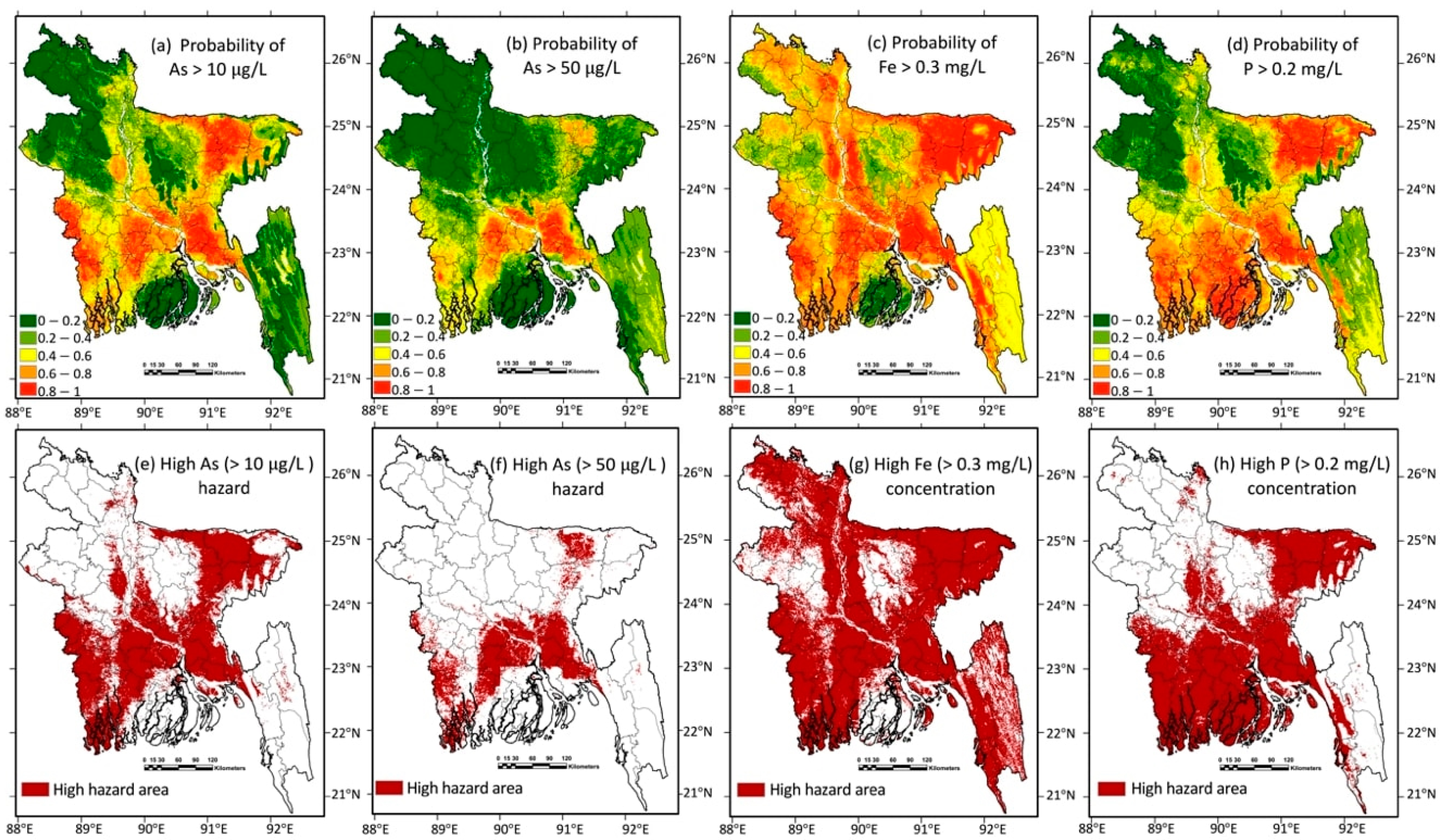
3.3. Distribution of Arsenic, Phosphorus, and Iron in Groundwater

The random forest model-generated probability maps for groundwater As, Fe, and P concentrations exceeding the selected concentration thresholds (10 μg/L or 50 μg/L for As, 0.3 mg/L for Fe, and 0.2 mg/L for P) are shown in Figure 1a–d, and these were converted into high-hazard/high-concentration maps (Figure 1e–h) using a default probability cutoff value of 0.5. The modelled distribution was broadly similar to that previously published by Tan et al. (2020) [59]; however, our models identified slightly more higher-probability zones in southwest (the Khulana region) and northeast (the Sylhet region) Bangladesh and slightly fewer high-probability zones in middle (the upper Dhaha region) Bangladesh. The new random forest models of the distribution of Fe and P (Figure 1g,h) were compared with the distribution of As > 10 μg/L (Figure 1e) in the groundwater. The predicted distribution of high-groundwater Fe (> 0.3 mg/L) had some similarities with the predicted distribution of high As, notwithstanding that the As and Fe were broadly inversely correlated (as shown in Figure S3). High-groundwater P zones occupy a large area in Bangladesh, especially including in some high-As areas, and this is not beneficial for groundwater As removal due to the increased likelihood of the competitive adsorption of P and As on the sorbents. The concentration thresholds of Fe and P in the separate random forest models were not selected based on the As remediation efficiency ratio, and the predicted separate distributions of As, Fe, and P were difficult to compare visually, highlighting the requirement for the further random forest prediction of the molar ratio [ Fe ] 1.8 [ P ] [ As ] .

3.4. Predicted Comparative Level of Arsenic Remediation Efficiency in Groundwater

The calculated (based on the DPHE/BGS (2001) data) [2] and modelled (this study) geographical distributions of the molar ratio [ Fe ] 1.8 [ P ] [ As ] are shown in Figure 2a,b. The probability map of the molar ratio [ Fe ] 1.8 [ P ] [ As ] exceeding the threshold value of 40 (Figure 2b) was converted into a comparatively high As remediation efficiency map by using a default probability cutoff value of 0.5, and the country-scale distribution of the comparative levels of “high” and “low” groundwater As remediation efficiency in Bangladesh is shown in Figure 2c. The predicted map of the comparative levels of As remediation efficiency was also combined with a predicted map of high As, and the high-As area was divided into two classifications (Figure 2d): (i) high As levels in the groundwater, which could likely be removed by the natural Fe in the groundwater using a sorption/co-precipitation-based technology (i.e., a high As and high comparative remediation efficiency level); and (ii) high As levels in the groundwater which likely could not be removed by the natural Fe in the groundwater (i.e., high As but low comparative remediation efficiency level), which could require the artificial addition of Fe to the groundwater.
The map of the comparatively high level of remediation efficiency suggested that the natural Fe concentrations were likely already sufficient (e.g., without the requirement for supplemental Fe) for removing the high As from the groundwater in north (the Rangpur region and the north Mymensingh region), middle (the north Dhaka region), and northeast (the Sylhet region) Bangladesh since the source water was geochemically compatible with the higher remediation efficiencies, especially the adsorption-based technologies. However, the high As levels in the south Dhaka, north Comilla, east Mymensingh, and west Sylhet regions may require supplementary Fe to be added improve the effectiveness of the As remediation strategies due to the insufficient natural Fe in the groundwater.
The predicted distribution of the comparative levels of As remediation efficiency provides pre-emptive guidance for informing appropriate and optimal groundwater (e.g., As) remediation selection. In high-As areas predicted to have comparatively low remediation efficiency (i.e., insufficient Fe), the addition of Fe may contribute to improved or optimised remediation efficiencies. In such cases, adding Fe(II) has a better removal performance than Fe(III) due to the oxidation of Fe(II) in aerated water, which generates reactive intermediates that can oxidise As(III) to As(V) [102]. The repetitive addition of Fe(II) can completely oxidise As(III) to As(V), which may have a stronger sorption capacity, facilitating removal by sorption on HFOs without oxidant additions [102].
Based on the good performance of the random forest models of the distribution of As, Fe, and P and the comparative level of the As remediation efficiency based on [ Fe ] 1.8 [ P ] [ As ] , we demonstrated that AI models (in this study, random forest machine learning models) can contribute to informing appropriate groundwater As remediation selection (e.g., the addition of Fe) at a large scale (e.g., the country scale) using the example of Bangladesh. The predicted distributions of the comparative levels of As remediation efficiencies can suggest whether high As levels can likely be removed naturally via naturally groundwater-sourced Fe or high As levels may require artificial Fe addition to be remediated in groundwater. However, for a specific groundwater well, well-specific testing is still required to select the optimal groundwater remediation approach due to the high spatial heterogeneity of the groundwater’s chemical constituents (e.g., As, Fe, and P).
Our predicted district-level proportions of 1 km × 1 km pixels of “As removal OK” ( [ Fe ] 1.8 [ P ] [ As ] > 40) was calculated and compared with the district-level measured well proportions of “As removal OK” calculated by Hug et al. (2008) using the same dataset [2] within 10–90 m depths (Table S2). There were significant differences in the modelled district-level proportions (%) of “As removal OK” between Hug’s approach (2008) [6], which was based entirely on samples measured in a particular district, and our approach presented here, which was based on random forest prediction on a km-square, pixel-by-pixel basis averaged without bias across an entire district. For example, for Meherpur district, Hug et al. (2008) [6] calculated approximately 23% of “As removal OK” based on 13 sampling data, while our modelled district-level proportion (%) of the "As removal OK" points was estimated to be approximately 85% based on modelling 783 1-km2 pixels. These differences provide a strong justification for our machine learning approach given that the samples in the DPHE/BGS National Hydrochemical Survey [2] dataset are not necessarily representative of each relevant district, nor are they representative of the whole sampled depth range, and thus, our more granular mapping approach on a km-square basis arguably adds substantial value. This comparison was also done for two different As concentration ranges (0–50 μg/L and >50 μg/L; Figure S7 and Table S2). It was found that for the As concentration range 0–50 μg/L, our predicted district-level proportion of pixels that were “As removal OK” tended to be higher than that in than Hug’s approach (2008) [6], and the difference between our modelling and Hug’s approach (2008) [6] for the As concentration range 0–50 μg/L was systematically larger than that for the concentration range As > 50 μg/L. However, the difference between our modelling and Hug’s approach (2008) for As > 50 μg/L was random.

3.5. Limitations

Although AI machine learning (random forest) models can contribute to informing the optimal remediation approach for groundwater As, site-specific water quality testing is still strongly recommended because of the limitations of this approach. Firstly, the potentially substantial local spatial heterogeneity of groundwater composition may not be adequately captured by a model. Secondly, in this study, the comparative remediation efficiency molar ratio only took into account the likely influence of the concentrations of Fe and P on the As remediation, whereas other water quality parameters (e.g., pH, organic matter, bicarbonate, and silicate concentrations) may also impact remediation efficiency and were not considered. Thirdly, other human factors (e.g., technology selection, regulatory and monitoring settings, socio-economic conditions, effectiveness (or otherwise) of the maintenance of field As removal units) may also critically contribute to groundwater As remediation efficiency. Fourthly, the environmental predictors used in the modelling were mainly related to the mobility, release, and enrichment of As in groundwater, and although these are likely somewhat related, consideration of additional environmental predictor parameters specifically associated with Fe and P might improve the AI model. Fifthly, particularly because the relationship between As removal efficiency and the molar ratio [ Fe ] 1.8 [ P ] [ As ] is complex (Figure S2), our machine learning model approach could be improved by better establishing and quantifying the dependence of source water chemistry on As removal efficiency (including via lab-based studies [103]). Lastly, the extent to which machine learning approaches may (or may not) be relevant to multiple hazards beyond groundwater As (e.g., contaminants with differing redox controls, such as U [47], or microbial pollutants) has not been investigated and would be an interesting area for further study.

4. Conclusions

AI machine learning (random forest) modelling has enabled the prediction of the potential effectiveness of source-water-chemistry-dependent sorption/co-precipitation-based groundwater As remediation systems at the 1 km2 scale in Bangladesh. The comparison between the predicted distributions of As, Fe, P, and the molar ratio [ Fe ] 1.8 [ P ] [ As ] in Bangladesh at the national scale indicated where high-groundwater As contamination may require the extra artificial addition of Fe to improve As remediation efficiency levels due to the predicted insufficient natural Fe levels in the groundwater. Whilst broadly consistent with previous district-scale models, our AI approach resulted in models with 100-fold greater granularity, importantly providing key added value as a decision support tool.
Although the study here was focused on machine learning for remediation selection for groundwater As in Bangladesh, the approach also has significant potential for future development across other regions and for other groundwater/soil contaminants, provided robust secondary chemical composition and environmental predictor datasets are available. Although machine learning models may help to inform appropriate groundwater remediation selection, such modelling does not intend to replace detailed and site-specific investigations of groundwater quality, particularly in areas with local spatial heterogeneity.
Using machine learning models to inform groundwater As remediation selection also provides substantial opportunities for further development, particularly where experimental or pilot-scale studies demonstrate relationships between the As or other contaminant removal efficiencies of particular remediation technologies and source water chemistry.

Supplementary Materials

The following supporting information can be downloaded at: https://www.mdpi.com/article/10.3390/w15203539/s1, Figure S1, Distribution of secondary groundwater composition data; Figure S2, Meta-analysis plots of As removal (% and absolute) versus the molar ratio ([Fe]—1.8 [P])/[As]; Figure S3, Bivariate plots of groundwater composition; Figure S4, District-level As remediation efficiency versus groundwater As > 50 µg/L; Figure S5, AUC curves; Figure S6, Normalised importance of the predictor variables; Figure S7, Comparison between the model predictions; Table S1, Description of the predictors used; Table S2, Bangladesh district-level comparison between this study and the study by Hug et al. (2008). Full caption details are provided in the Supplementary Information.

Author Contributions

Conceptualization, L.A.R., D.A.P. and R.W.; methodology, software, validation, and formal analysis, R.W.; data curation, R.W., L.A.R., A.R. and D.A.P.; writing—original draft preparation, R.W.; writing—review and editing, L.A.R., D.A.P. and A.R.; supervision and project administration, L.A.R. and D.A.P.; funding acquisition, L.A.R., D.A.P. and A.R. All authors have read and agreed to the published version of the manuscript.

Funding

This research was supported by the NERC Exploring Frontiers award (NE/X010813/1 to L.A.R. and D.A.P.), Department of Science and Technology (DST, India)—Newton Bhabha—Natural Environmental Research Council (NERC, UK)—Engineering and Physical Sciences Research Council (EPSRC, UK) Indo-UK Water Quality Programme award (NE/R003386/1 and DST/TM/INDO-UK/2K17/55(C) and 55(G)), 2018–2021, to DP et al. (see www.farganga.org, last accessed 1 October 2023); a University of Manchester-KTH Royal Institute of Technology-Stockholm University 2021–2022 seedcorn award to Co-PIs L.A.R., Bhattacharya, and Destouni and a Dame Kathleen Ollerenshaw Fellowship to L.A.R. A.R. acknowledges a University of Manchester-University of Melbourne dual PhD studentship. The authors thank their editor and the anonymous reviewers for their comments, which helped them to improve the manuscript.

Data Availability Statement

The data presented in this study not otherwise available from the references and organizations indicated in the text may be available on reasonable request from the corresponding author.

Conflicts of Interest

The authors declare no conflict of interest. The funders had no role in the design of the study; in the collection, analysis, or interpretation of the data; in the writing of the manuscript; or in the decision to publish the results.

References

  1. Mishra, B.; Kumar, P.; Saraswat, C.; Chakraborty, S.; Gautam, A. Water Security in a Changing Environment: Concept, Challenges and Solutions. Water 2021, 13, 490. [Google Scholar] [CrossRef]
  2. BGS; DPHE. Arsenic Contamination of Groundwater in Bangladesh; British Geological Survey: Keyworth, UK, 2001. [Google Scholar]
  3. WHO; UNICEF. Arsenic Primer—Guidance on the Investigation & Mitigation of Arsenic Contamination; WHO: New York, NY, USA, 2018. [Google Scholar]
  4. Khalid, S.; Shahid, M.; Bibi, I.; Natasha; Murtaza, B.; Tariq, T.Z.; Naz, R.; Shahzad, M.; Hussain, M.M.; Niazi, N.K. Global Arsenic Contamination of Groundwater, Soil and Food Crops and Health Impacts. In Global Arsenic Hazard; Niazi, N.K., Bibi, I., Aftab, T., Eds.; Environmental Science and Engineering; Springer International Publishing: Cham, Switzerland, 2023; pp. 13–33. ISBN 978-3-031-16359-3. [Google Scholar]
  5. Ravenscroft, P.; Brammer, H.; Richards, K.S. Arsenic Pollution: A Global Synthesis; RGS-IBG Book Series; Wiley-Blackwell: Chichester, UK; Malden, MA, USA, 2009; ISBN 978-1-4051-8602-5. [Google Scholar]
  6. Hug, S.J.; Leupin, O.X.; Berg, M. Bangladesh and Vietnam: Different Groundwater Compositions Require Different Approaches to Arsenic Mitigation. Environ. Sci. Technol. 2008, 42, 6318–6323. [Google Scholar] [CrossRef] [PubMed]
  7. Ahmed, M.F.; Ahuja, S.; Alauddin, M.; Hug, S.J.; Lloyd, J.R.; Pfaff, A.; Pichler, T.; Saltikov, C.; Stute, M.; van Geen, A. Ensuring Safe Drinking Water in Bangladesh. Science 2006, 314, 1687–1688. [Google Scholar] [CrossRef] [PubMed]
  8. IARC. Arsenic, Metals, Fibres and Dusts; IARC Working Group on the Evaluation of Carcinogenic Risks to Humans; International Agency for Research on Cancer: Lyon, France, 2012; Volume 100C, ISBN 978-92-832-0135-9. [Google Scholar]
  9. Chen, Y.; Ahsan, H. Cancer Burden from Arsenic in Drinking Water in Bangladesh. Am. J. Public Health 2004, 94, 741–744. [Google Scholar] [CrossRef] [PubMed]
  10. Chowdhury, U.K.; Biswas, B.K.; Chowdhury, T.R.; Samanta, G.; Mandal, B.K.; Basu, G.C.; Chanda, C.R.; Lodh, D.; Saha, K.C.; Mukherjee, S.K.; et al. Groundwater Arsenic Contamination in Bangladesh and West Bengal, India. Environ. Health Perspect. 2000, 108, 393–397. [Google Scholar] [CrossRef] [PubMed]
  11. Mondal, P.; Majumder, C.B.; Mohanty, B. Laboratory Based Approaches for Arsenic Remediation from Contaminated Water: Recent Developments. J. Hazard. Mater. 2006, 137, 464–479. [Google Scholar] [CrossRef] [PubMed]
  12. Ahmad, A.; Richards, L.A.; Bhattacharya, P. Arsenic Remediation of Drinking Water: An Overview. In Best Practice Guide on the Control of Arsenic in Drinking Water; Bhattacharya, P., Polya, D.A., Jovanovic, D., Eds.; IWA Publishing: London, UK, 2017; pp. 79–98. ISBN 978-1-78040-492-9. [Google Scholar]
  13. Dutta, N.; Gupta, A. Development of Arsenic Removal Unit with Electrocoagulation and Activated Alumina Sorption: Field Trial at Rural West Bengal, India. J. Water Process Eng. 2022, 49, 103013. [Google Scholar] [CrossRef]
  14. Kumar, A.; Joshi, H.; Kumar, A. Remediation of Arsenic by Metal/Metal Oxide Based Nanocomposites/Nanohybrids: Contamination Scenario in Groundwater, Practical Challenges, and Future Perspectives. Sep. Purif. Rev. 2021, 50, 283–314. [Google Scholar] [CrossRef]
  15. Irshad, S.; Xie, Z.; Mehmood, S.; Nawaz, A.; Ditta, A.; Mahmood, Q. Insights into Conventional and Recent Technologies for Arsenic Bioremediation: A Systematic Review. Environ. Sci. Pollut. Res. 2021, 28, 18870–18892. [Google Scholar] [CrossRef]
  16. Liu, R.; Qu, J. Review on Heterogeneous Oxidation and Adsorption for Arsenic Removal from Drinking Water. J. Environ. Sci. 2021, 110, 178–188. [Google Scholar] [CrossRef]
  17. Younger, P.L.; Coulton, R.H.; Froggatt, E.C. The Contribution of Science to Risk-Based Decision-Making: Lessons from the Development of Full-Scale Treatment Measures for Acidic Mine Waters at Wheal Jane, UK. Sci. Total Environ. 2005, 338, 137–154. [Google Scholar] [CrossRef]
  18. Bhattacharya, A.; Sahu, S.; Telu, V.; Duttagupta, S.; Sarkar, S.; Bhattacharya, J.; Mukherjee, A.; Ghosal, P.S. Neural Network and Random Forest-Based Analyses of the Performance of Community Drinking Water Arsenic Treatment Plants. Water 2021, 13, 3507. [Google Scholar] [CrossRef]
  19. Richards, L.A.; Wu, R.; Polya, D.A. Water Security in South Asia: The Potential Role of Artificial Intelligence in Supporting the Selection of Remediation Approached for Groundwater; Publisher: Denver, CO, USA, 2022. [Google Scholar]
  20. Hassan, K.M.; Fukuhara, T.; Hai, F.I.; Bari, Q.H.; Islam, K.M.S. Development of a Bio-Physicochemical Technique for Arsenic Removal from Groundwater. Desalination 2009, 249, 224–229. [Google Scholar] [CrossRef]
  21. Shafiquzzaman, M.; Azam, M.S.; Nakajima, J.; Bari, Q.H. Investigation of Arsenic Removal Performance by a Simple Iron Removal Ceramic Filter in Rural Households of Bangladesh. Desalination 2011, 265, 60–66. [Google Scholar] [CrossRef]
  22. Roberts, L.C.; Hug, S.J.; Ruettimann, T.; Billah, M.M.; Khan, A.W.; Rahman, M.T. Arsenic Removal with Iron(II) and Iron(III) in Waters with High Silicate and Phosphate Concentrations. Environ. Sci. Technol. 2004, 38, 307–315. [Google Scholar] [CrossRef] [PubMed]
  23. Pallier, V.; Feuillade-Cathalifaud, G.; Serpaud, B.; Bollinger, J.-C. Effect of Organic Matter on Arsenic Removal during Coagulation/Flocculation Treatment. J. Colloid Interface Sci. 2010, 342, 26–32. [Google Scholar] [CrossRef]
  24. Cornejo, L.; Lienqueo, H.; Arenas, M.; Acarapi, J.; Contreras, D.; Yáñez, J.; Mansilla, H.D. In Field Arsenic Removal from Natural Water by Zero-Valent Iron Assisted by Solar Radiation. Environ. Pollut. 2008, 156, 827–831. [Google Scholar] [CrossRef]
  25. Hasan, M.M.; Shafiquzzaman, M.; Nakajima, J.; Bari, Q.H. Application of a Simple Arsenic Removal Filter in a Rural Area of Bangladesh. Water Supply 2012, 12, 658–665. [Google Scholar] [CrossRef]
  26. Wu, K.; Liu, R.; Liu, H.; Chang, F.; Lan, H.; Qu, J. Arsenic Species Transformation and Transportation in Arsenic Removal by Fe-Mn Binary Oxide–Coated Diatomite: Pilot-Scale Field Study. J. Environ. Eng. 2011, 137, 1122–1127. [Google Scholar] [CrossRef]
  27. Sahai, N.; Lee, Y.J.; Xu, H.; Ciardelli, M.; Gaillard, J.-F. Role of Fe(II) and Phosphate in Arsenic Uptake by Coprecipitation. Geochim. Cosmochim. Acta 2007, 71, 3193–3210. [Google Scholar] [CrossRef]
  28. Bortun, A.; Bortun, M.; Pardini, J.; Khainakov, S.A.; García, J.R. Effect of Competitive Ions on the Arsenic Removal by Mesoporous Hydrous Zirconium Oxide from Drinking Water. Mater. Res. Bull. 2010, 45, 1628–1634. [Google Scholar] [CrossRef]
  29. De Klerk, R.J.; Jia, Y.; Daenzer, R.; Gomez, M.A.; Demopoulos, G.P. Continuous Circuit Coprecipitation of Arsenic(V) with Ferric Iron by Lime Neutralization: Process Parameter Effects on Arsenic Removal and Precipitate Quality. Hydrometallurgy 2012, 111–112, 65–72. [Google Scholar] [CrossRef]
  30. Senn, A.-C.; Kaegi, R.; Hug, S.J.; Hering, J.G.; Mangold, S.; Voegelin, A. Composition and Structure of Fe(III)-Precipitates Formed by Fe(II) Oxidation in Water at near-Neutral PH: Interdependent Effects of Phosphate, Silicate and Ca. Geochim. Cosmochim. Acta 2015, 162, 220–246. [Google Scholar] [CrossRef]
  31. Voegelin, A.; Kaegi, R.; Frommer, J.; Vantelon, D.; Hug, S.J. Effect of Phosphate, Silicate, and Ca on Fe(III)-Precipitates Formed in Aerated Fe(II)- and As(III)-Containing Water Studied by X-Ray Absorption Spectroscopy. Geochim. Cosmochim. Acta 2010, 74, 164–186. [Google Scholar] [CrossRef]
  32. Gao, Y.; Mucci, A. Acid Base Reactions, Phosphate and Arsenate Complexation, and Their Competitive Adsorption at the Surface of Goethite in 0.7 M NaCl Solution. Geochim. Cosmochim. Acta 2001, 65, 2361–2378. [Google Scholar] [CrossRef]
  33. Zeng, H.; Fisher, B.; Giammar, D.E. Individual and Competitive Adsorption of Arsenate and Phosphate to a High-Surface-Area Iron Oxide-Based Sorbent. Environ. Sci. Technol. 2008, 42, 147–152. [Google Scholar] [CrossRef]
  34. Biswas, A.; Gustafsson, J.P.; Neidhardt, H.; Halder, D.; Kundu, A.K.; Chatterjee, D.; Berner, Z.; Bhattacharya, P. Role of Competing Ions in the Mobilization of Arsenic in Groundwater of Bengal Basin: Insight from Surface Complexation Modeling. Water Res. 2014, 55, 30–39. [Google Scholar] [CrossRef]
  35. Manning, B.A.; Goldberg, S. Modeling Arsenate Competitive Adsorption on Kaolinite, Montmorillonite and Illite. Clays Clay Miner. 1996, 44, 609–623. [Google Scholar] [CrossRef]
  36. Youngran, J.; Fan, M.; Van Leeuwen, J.; Belczyk, J.F. Effect of Competing Solutes on Arsenic(V) Adsorption Using Iron and Aluminum Oxides. J. Environ. Sci. 2007, 19, 910–919. [Google Scholar] [CrossRef]
  37. Fytianos, K.; Voudrias, E.; Raikos, N. Modelling of Phosphorus Removal from Aqueous and Wastewater Samples Using Ferric Iron. Environ. Pollut. 1998, 101, 123–130. [Google Scholar] [CrossRef]
  38. Hongshao, Z.; Stanforth, R. Competitive Adsorption of Phosphate and Arsenate on Goethite. Environ. Sci. Technol. 2001, 35, 4753–4757. [Google Scholar] [CrossRef] [PubMed]
  39. Chowdhury, S.R.; Yanful, E.K. Arsenic and Chromium Removal by Mixed Magnetite–Maghemite Nanoparticles and the Effect of Phosphate on Removal. J. Environ. Manag. 2010, 91, 2238–2247. [Google Scholar] [CrossRef] [PubMed]
  40. Zhang, J.S.; Stanforth, R.; Pehkonen, S.O. Irreversible Adsorption of Methyl Arsenic, Arsenate, and Phosphate onto Goethite in Arsenic and Phosphate Binary Systems. J. Colloid Interface Sci. 2008, 317, 35–43. [Google Scholar] [CrossRef] [PubMed]
  41. Neidhardt, H.; Rudischer, S.; Eiche, E.; Schneider, M.; Stopelli, E.; Duyen, V.T.; Trang, P.T.K.; Viet, P.H.; Neumann, T.; Berg, M. Phosphate Immobilisation Dynamics and Interaction with Arsenic Sorption at Redox Transition Zones in Floodplain Aquifers: Insights from the Red River Delta, Vietnam. J. Hazard. Mater. 2021, 411, 125128. [Google Scholar] [CrossRef] [PubMed]
  42. Manning, B.A.; Goldberg, S. Modeling Competitive Adsorption of Arsenate with Phosphate and Molybdate on Oxide Minerals. Soil Sci. Soc. Am. J. 1996, 60, 121–131. [Google Scholar] [CrossRef]
  43. Han, Y.-S.; Park, J.-H.; Min, Y.; Lim, D.-H. Competitive Adsorption between Phosphate and Arsenic in Soil Containing Iron Sulfide: XAS Experiment and DFT Calculation Approaches. Chem. Eng. J. 2020, 397, 125426. [Google Scholar] [CrossRef]
  44. Tiberg, C.; Sjöstedt, C.; Eriksson, A.K.; Klysubun, W.; Gustafsson, J.P. Phosphate Competition with Arsenate on Poorly Crystalline Iron and Aluminum (Hydr)Oxide Mixtures. Chemosphere 2020, 255, 126937. [Google Scholar] [CrossRef] [PubMed]
  45. Niazi, N.K.; Burton, E.D. Arsenic Sorption to Nanoparticulate Mackinawite (FeS): An Examination of Phosphate Competition. Environ. Pollut. 2016, 218, 111–117. [Google Scholar] [CrossRef]
  46. Voegelin, A.; Senn, A.-C.; Kaegi, R.; Hug, S.J.; Mangold, S. Dynamic Fe-Precipitate Formation Induced by Fe(II) Oxidation in Aerated Phosphate-Containing Water. Geochim. Cosmochim. Acta 2013, 117, 216–231. [Google Scholar] [CrossRef]
  47. Richards, L.A.; Kumar, A.; Shankar, P.; Gaurav, A.; Ghosh, A.; Polya, D.A. Distribution and Geochemical Controls of Arsenic and Uranium in Groundwater-Derived Drinking Water in Bihar, India. Int. J. Environ. Res. Public Health 2020, 17, 2500. [Google Scholar] [CrossRef]
  48. Podgorski, J.; Berg, M. Global Threat of Arsenic in Groundwater. Science 2020, 368, 845–850. [Google Scholar] [CrossRef] [PubMed]
  49. Amini, M.; Abbaspour, K.C.; Berg, M.; Winkel, L.; Hug, S.J.; Hoehn, E.; Yang, H.; Johnson, C.A. Statistical Modeling of Global Geogenic Arsenic Contamination in Groundwater. Environ. Sci. Technol. 2008, 42, 3669–3675. [Google Scholar] [CrossRef] [PubMed]
  50. Ayotte, J.D.; Medalie, L.; Qi, S.L.; Backer, L.C.; Nolan, B.T. Estimating the High-Arsenic Domestic-Well Population in the Conterminous United States. Environ. Sci. Technol. 2017, 51, 12443–12454. [Google Scholar] [CrossRef] [PubMed]
  51. Ayotte, J.D.; Montgomery, D.L.; Flanagan, S.M.; Robinson, K.W. Arsenic in Groundwater in Eastern New England: Occurrence, Controls, and Human Health Implications. Environ. Sci. Technol. 2003, 37, 2075–2083. [Google Scholar] [CrossRef]
  52. Winkel, L.; Berg, M.; Amini, M.; Hug, S.J.; Annette Johnson, C. Predicting Groundwater Arsenic Contamination in Southeast Asia from Surface Parameters. Nat. Geosci. 2008, 1, 536–542. [Google Scholar] [CrossRef]
  53. Sovann, C.; Polya, D.A. Improved Groundwater Geogenic Arsenic Hazard Map for Cambodia. Environ. Chem. 2014, 11, 595. [Google Scholar] [CrossRef]
  54. Podgorski, J.E.; Eqani, S.A.M.A.S.; Khanam, T.; Ullah, R.; Shen, H.; Berg, M. Extensive Arsenic Contamination in High-PH Unconfined Aquifers in the Indus Valley. Sci. Adv. 2017, 3, e1700935. [Google Scholar] [CrossRef]
  55. Mukherjee, A.; Sarkar, S.; Chakraborty, M.; Duttagupta, S.; Bhattacharya, A.; Saha, D.; Bhattacharya, P.; Mitra, A.; Gupta, S. Occurrence, Predictors and Hazards of Elevated Groundwater Arsenic across India through Field Observations and Regional-Scale AI-Based Modeling. Sci. Total Environ. 2021, 759, 143511. [Google Scholar] [CrossRef]
  56. Wu, R.; Xu, L.; Polya, D.A. Groundwater Arsenic-Attributable Cardiovascular Disease (CVD) Mortality Risks in India. Water 2021, 13, 2232. [Google Scholar] [CrossRef]
  57. Podgorski, J.; Wu, R.; Chakravorty, B.; Polya, D.A. Groundwater Arsenic Distribution in India by Machine Learning Geospatial Modeling. Int. J. Environ. Res. Public Health 2020, 17, 7119. [Google Scholar] [CrossRef]
  58. Wu, R.; Alvareda, E.; Polya, D.; Blanco, G.; Gamazo, P. Distribution of Groundwater Arsenic in Uruguay Using Hybrid Machine Learning and Expert System Approaches. Water 2021, 13, 527. [Google Scholar] [CrossRef]
  59. Tan, Z.; Yang, Q.; Zheng, Y. Machine Learning Models of Groundwater Arsenic Spatial Distribution in Bangladesh: Influence of Holocene Sediment Depositional History. Environ. Sci. Technol. 2020, 54, 9454–9463. [Google Scholar] [CrossRef] [PubMed]
  60. Rodríguez-Lado, L.; Sun, G.; Berg, M.; Zhang, Q.; Xue, H.; Zheng, Q.; Johnson, C.A. Groundwater Arsenic Contamination Throughout China. Science 2013, 341, 866–868. [Google Scholar] [CrossRef]
  61. Bretzler, A.; Lalanne, F.; Nikiema, J.; Podgorski, J.; Pfenninger, N.; Berg, M.; Schirmer, M. Groundwater Arsenic Contamination in Burkina Faso, West Africa: Predicting and Verifying Regions at Risk. Sci. Total Environ. 2017, 584–585, 958–970. [Google Scholar] [CrossRef] [PubMed]
  62. Kumar, S.; Pati, J. Assessment of Groundwater Arsenic Contamination Using Machine Learning in Varanasi, Uttar Pradesh, India. J. Water Health 2022, 20, 829–848. [Google Scholar] [CrossRef]
  63. Wu, R.; Podgorski, J.; Berg, M.; Polya, D.A. Geostatistical Model of the Spatial Distribution of Arsenic in Groundwaters in Gujarat State, India. Environ. Geochem. Health 2021, 43, 2649–2664. [Google Scholar] [CrossRef]
  64. Ruidas, D.; Pal, S.C.; Towfiqul Islam, A.R.M.; Saha, A. Hydrogeochemical Evaluation of Groundwater Aquifers and Associated Health Hazard Risk Mapping Using Ensemble Data Driven Model in a Water Scares Plateau Region of Eastern India. Expo Health 2023, 15, 113–131. [Google Scholar] [CrossRef]
  65. Richards, L.A.; Parashar, N.; Kumari, R.; Kumar, A.; Mondal, D.; Ghosh, A.; Polya, D.A. Household and Community Systems for Groundwater Remediation in Bihar, India: Arsenic and Inorganic Contaminant Removal, Controls and Implications for Remediation Selection. Sci. Total Environ. 2022, 830, 154580. [Google Scholar] [CrossRef]
  66. Smith, A.H.; Lingas, E.O.; Rahman, M. Contamination of Drinking-Water by Arsenic in Bangladesh: A Public Health Emergency. Bull. World Health Organ. 2000, 78, 1093–1103. [Google Scholar]
  67. Ahmad, S.A.; Khan, M.A.; Faruquee, M.H.; Dutta, S.; Tani, M.; Kobayashi, M.; Shinohara, H. Arsenicosis: Nutrition and Socioeconomic Factors. J. Pre. Soc. Med. 2012, 31, 51–62. [Google Scholar]
  68. Flora, S.J.S. (Ed.) Handbook of Arsenic Toxicology; Academic Press: London, UK, 2015; ISBN 978-0-12-418688-0. [Google Scholar]
  69. Ahmad, S.A.; Khan, M.H.; Haque, M. Arsenic Contamination in Groundwater in Bangladesh: Implications and Challenges for Healthcare Policy. Risk Manag. Healthc. Policy 2018, 11, 251–261. [Google Scholar] [CrossRef] [PubMed]
  70. UNICEF. Drinking Water Quality in Bangladesh; UNICEF: New York, NY, USA, 2018. [Google Scholar]
  71. EPA. Drinking Water Regulations and Contaminants.; EPA: Washington, DC, USA, 2022. [Google Scholar]
  72. Smedley, P.L.; Kinniburgh, D.G. A Review of the Source, Behaviour and Distribution of Arsenic in Natural Waters. Appl. Geochem. 2002, 17, 517–568. [Google Scholar] [CrossRef]
  73. Islam, F.S.; Gault, A.G.; Boothman, C.; Polya, D.A.; Charnock, J.M.; Chatterjee, D.; Lloyd, J.R. Role of Metal-Reducing Bacteria in Arsenic Release from Bengal Delta Sediments. Nature 2004, 430, 68–71. [Google Scholar] [CrossRef]
  74. McArthur, J.M.; Banerjee, D.M.; Hudson-Edwards, K.A.; Mishra, R.; Purohit, R.; Ravenscroft, P.; Cronin, A.; Howarth, R.J.; Chatterjee, A.; Talukder, T.; et al. Natural Organic Matter in Sedimentary Basins and Its Relation to Arsenic in Anoxic Ground Water: The Example of West Bengal and Its Worldwide Implications. Appl. Geochem. 2004, 19, 1255–1293. [Google Scholar] [CrossRef]
  75. Charlet, L.; Polya, D.A. Arsenic in Shallow, Reducing Groundwaters in Southern Asia: An Environmental Health Disaster. Elements 2006, 2, 91–96. [Google Scholar] [CrossRef]
  76. Polya, D.; Charlet, L. Rising Arsenic Risk? Nat. Geosci. 2009, 2, 383–384. [Google Scholar] [CrossRef]
  77. Polya, D.A.; Middleton, D.R.S. Arsenic in Drinking Water: Sources & Human Exposure. In Best Practice Guide on the Control of Arsenic in Drinking Water; Bhattacharya, P., Polya, D.A., Jovanovic, D., Eds.; IWA Publishing: London, UK, 2017; pp. 1–23. ISBN 978-1-78040-492-9. [Google Scholar]
  78. Polya, D.A.; Sparrenbom, C.; Datta, S.; Guo, H. Groundwater Arsenic Biogeochemistry—Key Questions and Use of Tracers to Understand Arsenic-Prone Groundwater Systems. Geosci. Front. 2019, 10, 1635–1641. [Google Scholar] [CrossRef]
  79. Polya, D.A.; Xu, L.; Launder, J.; Gooddy, D.C.; Ascott, M. Distribution of Arsenic Hazard in Public Water Supplies in the United Kingdom—Methods, Implications for Health Risks and Recommendations. In Environmental Arsenic in a Changing World; CRC Press: London, UK, 2019; pp. 22–25. ISBN 978-1-351-04663-3. [Google Scholar]
  80. Trabucco, A.; Zomer, R.J. Global Soil Water Balance Geospatial Database. CGIAR Consortium for Spatial Information, 2010. CGIAR-CSI GeoPortal. Available online: https://cgiarcsi.community/ (accessed on 22 March 2019).
  81. Trabucco, A.; Zomer, R.J. Global Aridity Index (Global-Aridity) and Global Potential Evapo-Transpiration (Global- PET) Geospatial Database. CGIAR Consortium for Spatial Information, 2009. CGIAR-CSI GeoPortal. Available online: https://cgiarcsi.community/ (accessed on 18 February 2019).
  82. Hengl, T. Global Landform and Lithology Class at 250 m Based on the USGS Global Ecosystem Map. 2018. Available online: https://zenodo.org/record/1464846 (accessed on 20 February 2021).
  83. Hengl, T.; Mendes de Jesus, J.; Heuvelink, G.B.M.; Ruiperez Gonzalez, M.; Kilibarda, M.; Blagotić, A.; Shangguan, W.; Wright, M.N.; Geng, X.; Bauer-Marschallinger, B.; et al. SoilGrids250m: Global Gridded Soil Information Based on Machine Learning. PLoS ONE 2017, 12, e0169748. [Google Scholar] [CrossRef]
  84. Pelletier, J.D.; Broxton, P.D.; Hazenberg, P.; Zeng, X.; Troch, P.A.; Niu, G.; Williams, Z.C.; Brunke, M.A.; Gochis, D. Global 1-Km Gridded Thickness of Soil, Regolith, and Sedimentary Deposit Layers; ORNL DAAC: Oak Ridge, TN, USA, 2016. [Google Scholar] [CrossRef]
  85. Fan, Y.; Li, H.; Miguez-Macho, G. Global Patterns of Groundwater Table Depth. Science 2013, 339, 940–943. [Google Scholar] [CrossRef]
  86. Friedl, M.A.; Sulla-Menashe, D.; Tan, B.; Schneider, A.; Ramankutty, N.; Sibley, A.; Huang, X. MODIS Collection 5 Global Land Cover: Algorithm Refinements and Characterization of New Datasets. Remote Sens. Environ. 2010, 114, 168–182. [Google Scholar] [CrossRef]
  87. Earth Resources Observation and Science (EROS) Center. Global 30 Arc-Second Elevation (GTOPO30). 2017. Available online: https://www.usgs.gov/centers/eros/science/usgs-eros-archive-digital-elevation-global-30-arc-second-elevation-gtopo30 (accessed on 1 October 2019).
  88. Breiman, L. Random Forests. Mach. Learn. 2001, 45, 5–32. [Google Scholar] [CrossRef]
  89. Zhou, X.; Lu, P.; Zheng, Z.; Tolliver, D.; Keramati, A. Accident Prediction Accuracy Assessment for Highway-Rail Grade Crossings Using Random Forest Algorithm Compared with Decision Tree. Reliab. Eng. Syst. Saf. 2020, 200, 106931. [Google Scholar] [CrossRef]
  90. Wielenga, D. Identifying and Overcoming Common Data Mining Mistakes. In SAS Global Forum; SAS Institute Inc.: Cary, NC, USA, 2007. [Google Scholar]
  91. Meng, X.; Korfiatis, G.P.; Christodoulatos, C.; Bang, S. Treatment of Arsenic in Bangladesh Well Water Using a Household Co-Precipitation and Filtration System. Water Res. 2001, 35, 2805–2810. [Google Scholar] [CrossRef]
  92. Genç-Fuhrman, H.; Bregnhøj, H.; McConchie, D. Arsenate Removal from Water Using Sand–Red Mud Columns. Water Res. 2005, 39, 2944–2954. [Google Scholar] [CrossRef] [PubMed]
  93. Tyrovola, K.; Nikolaidis, N.P.; Veranis, N.; Kallithrakas-Kontos, N.; Koulouridakis, P.E. Arsenic Removal from Geothermal Waters with Zero-Valent Iron—Effect of Temperature, Phosphate and Nitrate. Water Res. 2006, 40, 2375–2386. [Google Scholar] [CrossRef] [PubMed]
  94. Ciardelli, M.C.; Xu, H.; Sahai, N. Role of Fe(II), Phosphate, Silicate, Sulfate, and Carbonate in Arsenic Uptake by Coprecipitation in Synthetic and Natural Groundwater. Water Res. 2008, 42, 615–624. [Google Scholar] [CrossRef]
  95. Guan, X.; Dong, H.; Ma, J.; Jiang, L. Removal of Arsenic from Water: Effects of Competing Anions on As(III) Removal in KMnO4–Fe(II) Process. Water Res. 2009, 43, 3891–3899. [Google Scholar] [CrossRef]
  96. Chiew, H.; Sampson, M.L.; Huch, S.; Ken, S.; Bostick, B.C. Effect of Groundwater Iron and Phosphate on the Efficacy of Arsenic Removal by Iron-Amended BioSand Filters. Environ. Sci. Technol. 2009, 43, 6295–6300. [Google Scholar] [CrossRef]
  97. Martinson, C.A.; Reddy, K.J. Adsorption of Arsenic(III) and Arsenic(V) by Cupric Oxide Nanoparticles. J. Colloid Interface Sci. 2009, 336, 406–411. [Google Scholar] [CrossRef]
  98. Van Halem, D.; Olivero, S.; de Vet, W.W.J.M.; Verberk, J.Q.J.C.; Amy, G.L.; van Dijk, J.C. Subsurface Iron and Arsenic Removal for Shallow Tube Well Drinking Water Supply in Rural Bangladesh. Water Res. 2010, 44, 5761–5769. [Google Scholar] [CrossRef]
  99. Lakshmanan, D.; Clifford, D.A.; Samanta, G. Comparative Study of Arsenic Removal by Iron Using Electrocoagulation and Chemical Coagulation. Water Res. 2010, 44, 5641–5652. [Google Scholar] [CrossRef]
  100. Nitzsche, K.S.; Lan, V.M.; Trang, P.T.K.; Viet, P.H.; Berg, M.; Voegelin, A.; Planer-Friedrich, B.; Zahoransky, J.; Müller, S.-K.; Byrne, J.M.; et al. Arsenic Removal from Drinking Water by a Household Sand Filter in Vietnam—Effect of Filter Usage Practices on Arsenic Removal Efficiency and Microbiological Water Quality. Sci. Total Environ. 2015, 502, 526–536. [Google Scholar] [CrossRef] [PubMed]
  101. Annaduzzaman, M.; Rietveld, L.C.; Hoque, B.A.; van Halem, D. Sequential Fe2+ Oxidation to Mitigate the Inhibiting Effect of Phosphate and Silicate on Arsenic Removal. Groundw. Sustain. Dev. 2022, 17, 100749. [Google Scholar] [CrossRef]
  102. Leupin, O.X.; Hug, S.J. Oxidation and Removal of Arsenic (III) from Aerated Groundwater by Filtration through Sand and Zero-Valent Iron. Water Res. 2005, 39, 1729–1740. [Google Scholar] [CrossRef] [PubMed]
  103. Ali, I.; Gupta, V.K. Advances in Water Treatment by Adsorption Technology. Nat. Protoc. 2006, 1, 2661–2667. [Google Scholar] [CrossRef]
Figure 1. Random forest models of the groundwater As, Fe, and P concentrations in Bangladesh. (a) Probability map of the groundwater As concentrations exceeding 10 μg/L. (b) Probability map of the groundwater As concentrations exceeding 50 μg/L. (c) Probability map of the groundwater Fe concentrations exceeding 0.3 mg/L. (d) Probability map of the groundwater P concentrations exceeding 0.2 mg/L. (e) Map of high-hazard As (>10 μg/L) areas. (f) Map of high-hazard As (>50 μg/L) areas. (g) Map of high-concentration Fe (>0.3 mg/L) areas. (h) Map of high-concentration P (>0.2 mg/L) areas. All high-hazard areas were defined by a default probability-exceeding cutoff value of 0.5.
Water 15 03539 g001
Figure 2. Random forest model of the distribution of the predicted high and low potential efficiencies of the sorption/co-precipitation-based groundwater As remediation systems in Bangladesh. (a) The molar ratio [ Fe ] 1.8 [ P ] [ As ]   calculated from the secondary data [2] for As, Fe, and P. (b) Map of the random-forest-modelled probability of the molar ratio [ Fe ] 1.8 [ P ] [ As ] > 40. (c) Map of the areas of the modelled high-potential As remediation efficiency (green) (defined by a default probability-exceeding cutoff value of 0.5). (d) Modelled maps of high-groundwater As areas with contrasting (i) predicted high-potential groundwater As remediation efficiency (yellow) and (ii) predicted low-potential groundwater As remediation efficiency for which the addition of Fe may be indicated to improve effectiveness (red).
Water 15 03539 g002
Disclaimer/Publisher’s Note: The statements, opinions and data contained in all publications are solely those of the individual author(s) and contributor(s) and not of MDPI and/or the editor(s). MDPI and/or the editor(s) disclaim responsibility for any injury to people or property resulting from any ideas, methods, instructions or products referred to in the content.

