

Machine Learning Algorithms for Predicting the Water Quality Index

 ,
,  , ,
, ,
Abstract
:1. Introduction
2. Materials and Methods
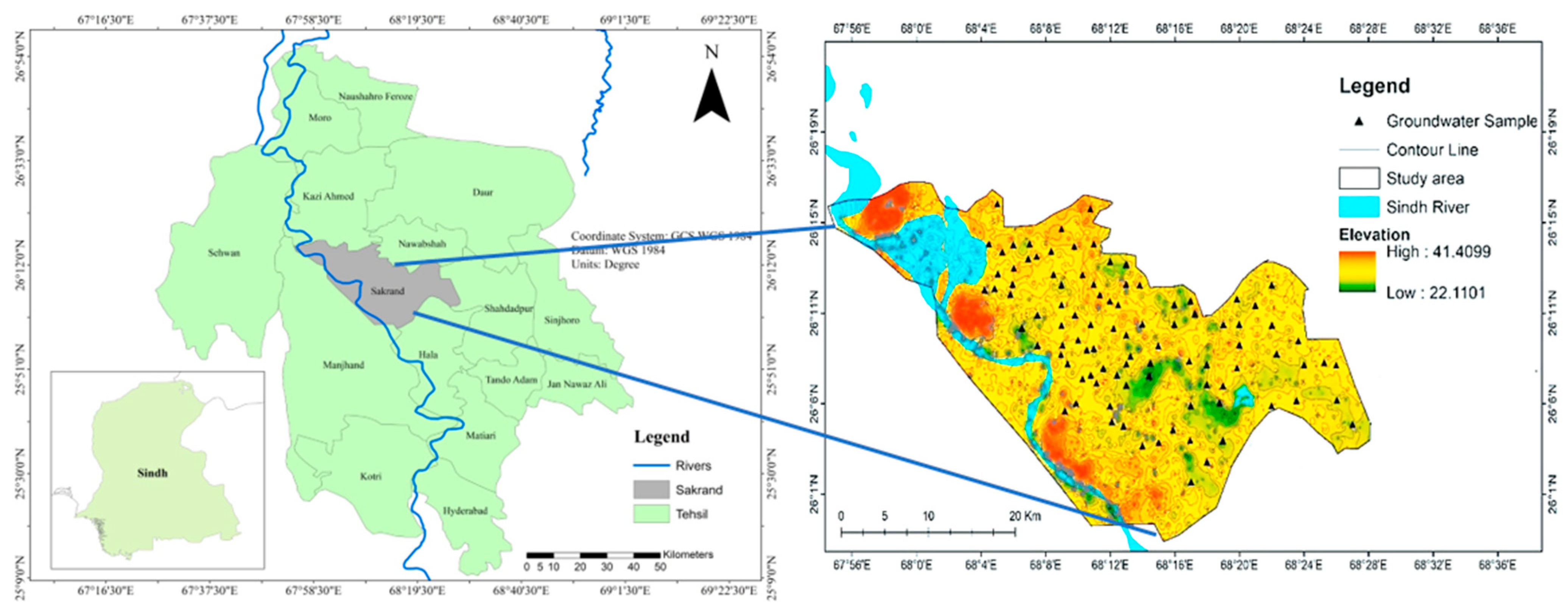
2.1. Description of the Study Area
2.2. Sample Collection and Analysis
2.3. Water Quality Index (WQI) of Groundwater
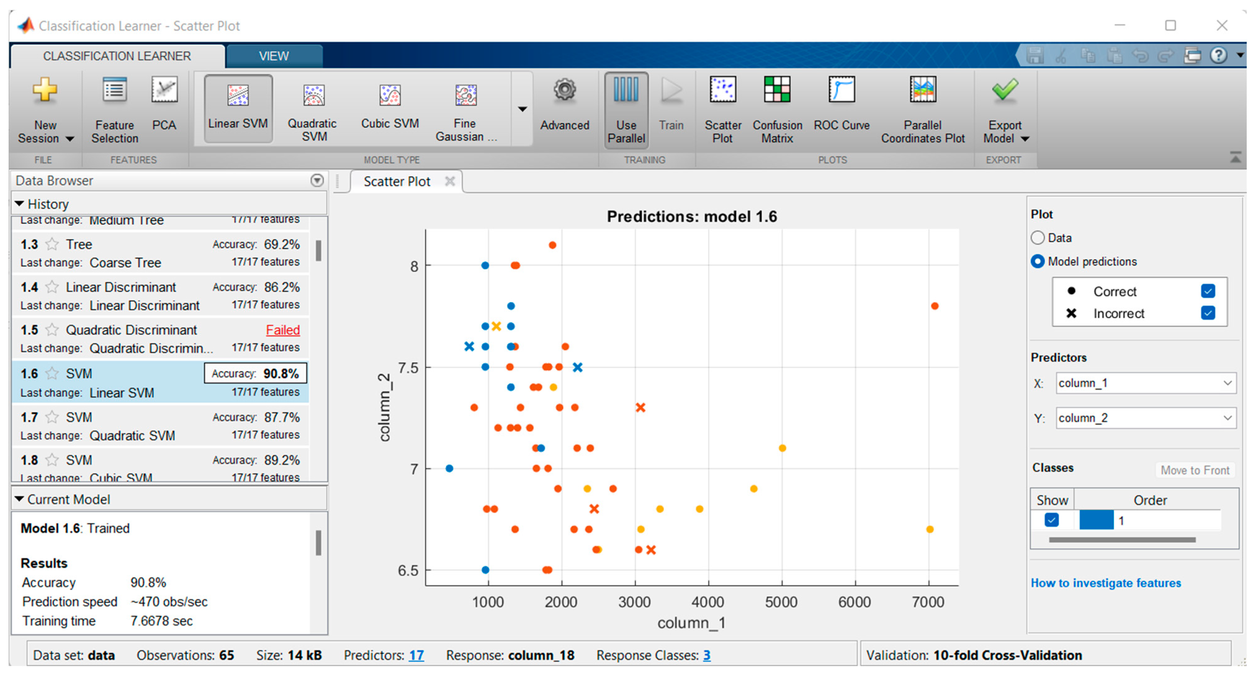
3. Classification Learner
3.1. Training Results of Classification Learner
- -
- There are not enough relevant and informative features. Thus, the classifiers struggle to make accurate predictions.
- -
- The training data are imbalanced, leading to one class having significantly more instances than the others.
- -
- When a classifier learns too much from the training data and cannot generalize effectively to new data; this might occur if the model is complicated or the training set contains noise.
- -
- When a classifier is too simple and fails to capture the underlying patterns in the data; this can happen if the model is not complex enough or if there are insufficient training data.
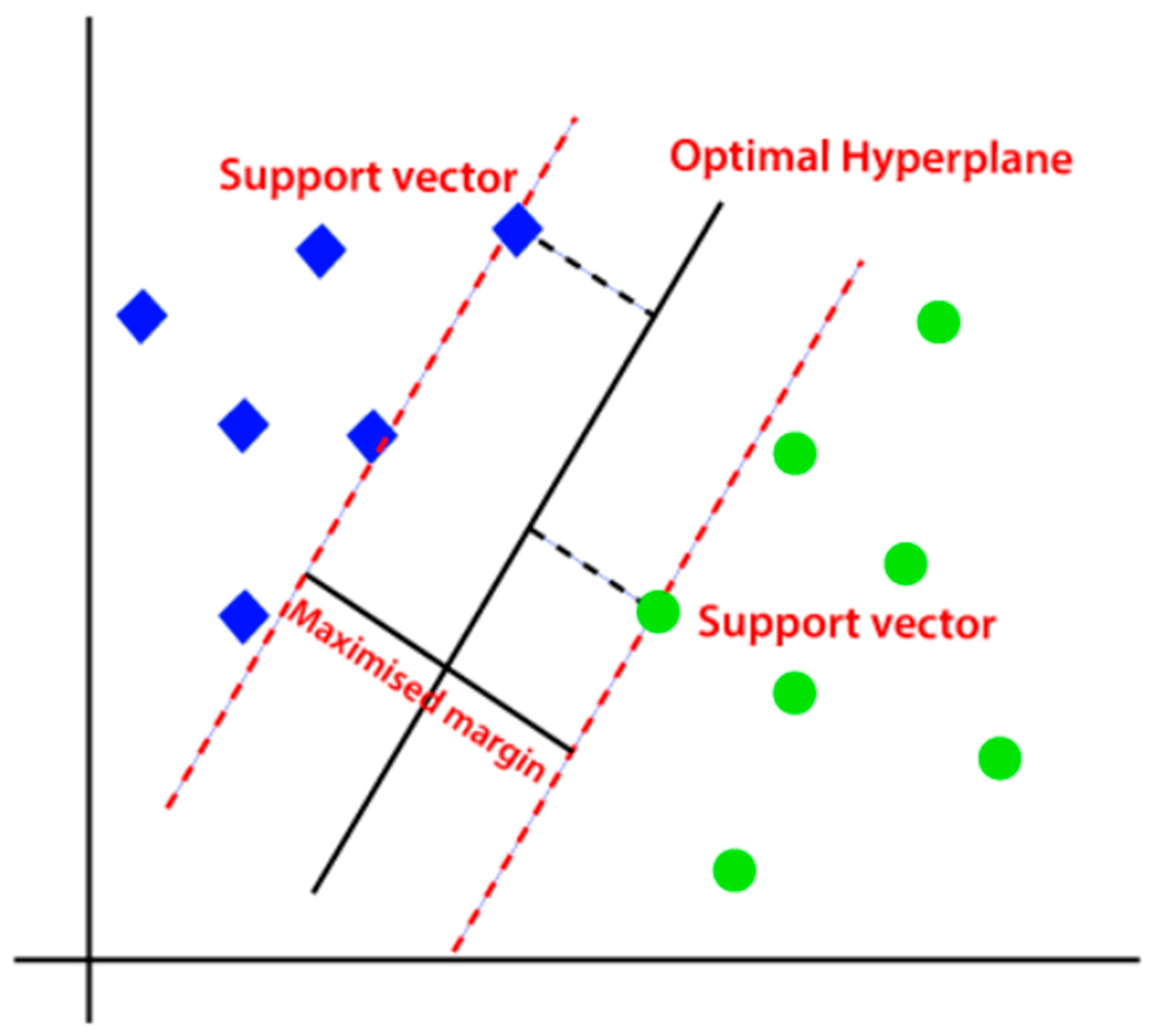
3.2. Linear Support Vector Machine (LSVM)
4. Results and Discussion
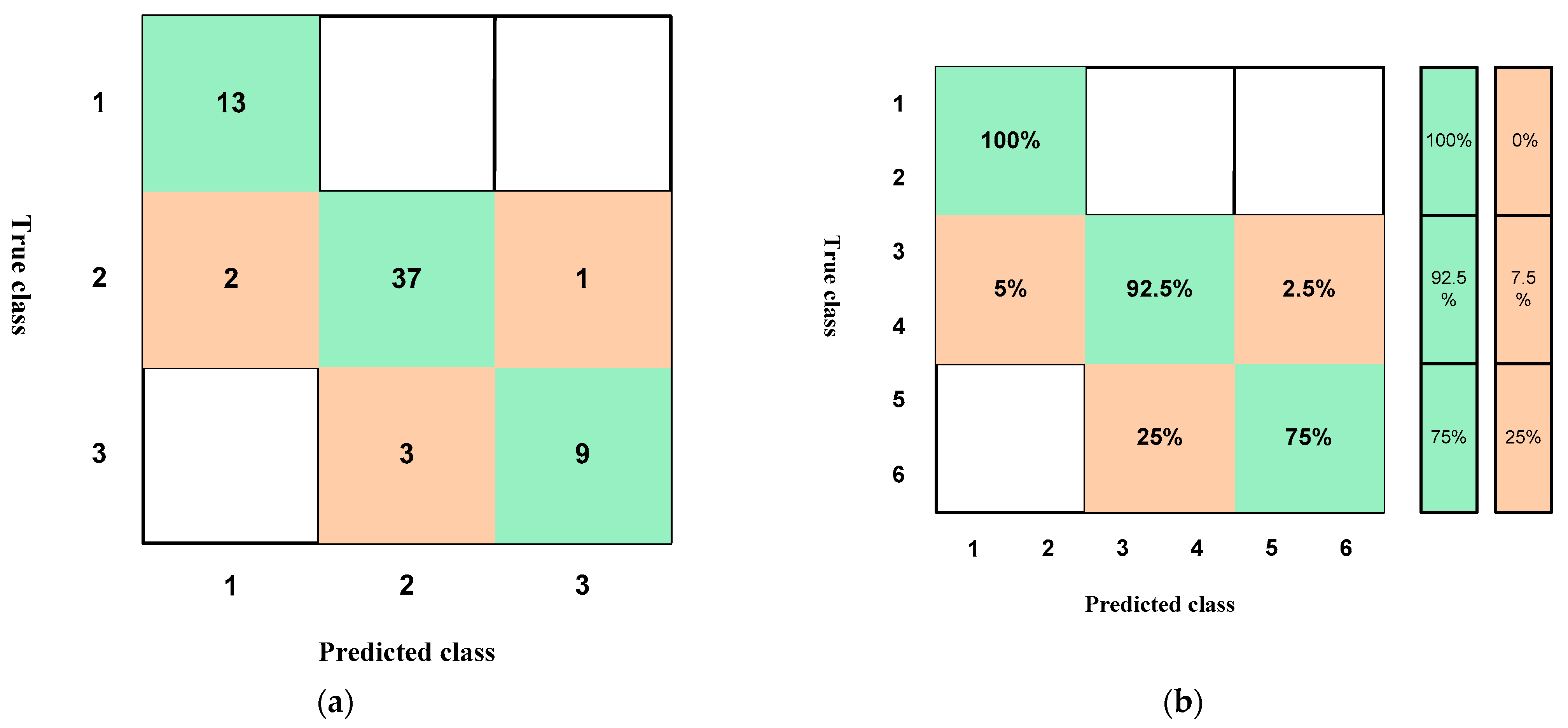
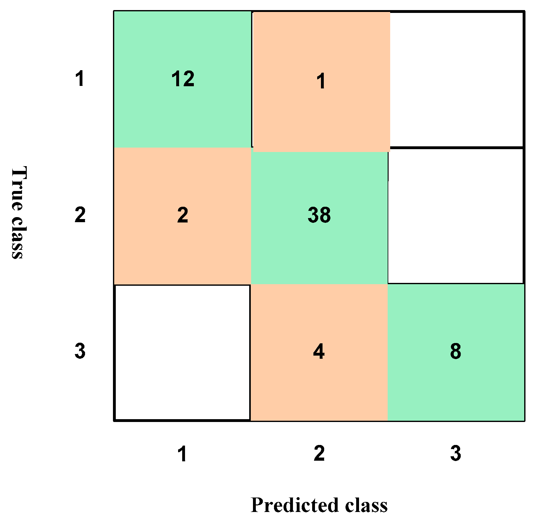
4.1. Results According to the Training of the Raw Data
4.2. Results According to the Training of the Normalization of the Data
5. Conclusions
Author Contributions
Funding
Institutional Review Board Statement
Informed Consent Statement
Data Availability Statement
Acknowledgments
Conflicts of Interest
References
- Dilpazeer, F.; Munir, M.; Baloch, M.Y.J.; Shafiq, I.; Iqbal, J.; Saeed, M.; Abbas, M.M.; Shafique, S.; Aziz, K.H.H.; Mustafa, A.; et al. A Comprehensive Review of the Latest Advancements in Controlling Arsenic Contaminants in Groundwater. Water 2023, 15, 478. [Google Scholar] [CrossRef]
- Jat Baloch, M.Y.; Zhang, W.; Zhang, D.; Al Shoumik, B.A.; Iqbal, J.; Li, S.; Chai, J.; Farooq, M.A.; Parkash, A. Evolution Mechanism of Arsenic Enrichment in Groundwater and Associated Health Risks in Southern Punjab, Pakistan. Int. J. Environ. Res. Public Health 2022, 19, 13325. [Google Scholar] [CrossRef]
- Li, S.; Zhang, W.; Zhang, D.; Xiu, W.; Wu, S.; Chai, J.; Ma, J.; Baloch, M.Y.J.; Sun, S.; Yang, Y. Migration risk of Escherichia coli O157: H7 in unsaturated porous media in response to different colloid types and compositions. Environ. Pollut. 2023, 323, 121282. [Google Scholar] [CrossRef] [PubMed]
- Baloch, M.Y.J.; Talpur, S.A.; Talpur, H.A.; Iqbal, J.; Mangi, S.H.; Memon, S. Effects of Arsenic Toxicity on the Environment and Its Remediation Techniques: A Review. J. Water Environ. Technol. 2020, 18, 275–289. [Google Scholar] [CrossRef]
- Tariq, A.; Mumtaz, F.; Zeng, X.; Baloch, M.Y.J.; Moazzam, M.F.U. Spatio-temporal variation of seasonal heat islands mapping of Pakistan during 2000–2019, using day-time and night-time land surface temperatures MODIS and meteorological stations data. Remote Sens. Appl. Soc. Environ. 2022, 27, 100779. [Google Scholar] [CrossRef]
- Tariq, A.; Ali, S.; Basit, I.; Jamil, A.; Farmonov, N.; Khorrami, B.; Khan, M.M.; Sadri, S.; Baloch, M.Y.J.; Islam, F. Terrestrial and groundwater storage characteristics and their quantification in the Chitral (Pakistan) and Kabul (Afghanistan) river basins using GRACE/GRACE-FO satellite data. Groundw. Sustain. Dev. 2023, 23, 100990. [Google Scholar] [CrossRef]
- Jat Baloch, M.Y.; Su, C.; Talpur, S.A.; Iqbal, J.; Bajwa, K. Arsenic Removal from Groundwater Using Iron Pyrite: Influence Factors and Removal Mechanism. J. Earth Sci. 2023, 34, 857–867. [Google Scholar] [CrossRef]
- Stojanović Bjelić, L.; Ilić, P.; Nešković Markić, D.; Ilić, S.; Popović, Z.; Mrazovac Kurilić, S.; Mihajlović, D.; Farooqi, Z.; Jat Baloch, M.; Mohamed, M. Contamination in water and ecological risk of heavy metals near a coal mine and a thermal power plant (republic of srpska, bosnia and herzegovina). Appl. Ecol. Environ. Res. 2023, 21, 3807–3822. [Google Scholar]
- Jat Baloch, M.Y.; Zhang, W.; Chai, J.; Li, S.; Alqurashi, M.; Rehman, G.; Tariq, A.; Talpur, S.A.; Iqbal, J.; Munir, M.; et al. Shallow groundwater quality assessment and its suitability analysis for drinking and irrigation purposes. Water 2021, 13, 3361. [Google Scholar] [CrossRef]
- Baloch, M.Y.J.; Mangi, S.H. Treatment of synthetic greywater by using banana, orange and sapodilla peels as a low cost activated carbon. J. Mater. Environ. Sci. 2019, 10, 966–986. [Google Scholar]
- Kumar, R.; Parkash, A.; Almani, S.; Baloch, M.Y.J.; Khan, R.; Soomro, S.A. Synthesis of porous cobalt oxide nanosheets: Highly sensitive sensors for the detection of hydrazine. Funct. Compos. Struct. 2022, 4, 035002. [Google Scholar] [CrossRef]
- Zhang, W.; Chai, J.; Li, S.; Wang, X.; Wu, S.; Liang, Z.; Baloch, M.Y.J.; Silva, L.F.; Zhang, D. Physiological characteristics, geochemical properties and hydrological variables influencing pathogen migration in subsurface system: What we know or not? Geosci. Front. 2022, 13, 101346. [Google Scholar] [CrossRef]
- Zhang, W.; Zhu, Y.; Gu, R.; Liang, Z.; Xu, W.; Jat Baloch, M.Y. Health Risk Assessment during In Situ Remediation of Cr (VI)-Contaminated Groundwater by Permeable Reactive Barriers: A Field-Scale Study. Int. J. Environ. Res. Public Health 2022, 19, 13079. [Google Scholar] [CrossRef] [PubMed]
- Iqbal, J.; Su, C.; Wang, M.; Abbas, H.; Baloch, M.Y.J.; Ghani, J.; Ullah, Z.; Huq, M.E. Groundwater fluoride and nitrate contamination and associated human health risk assessment in South Punjab, Pakistan. Environ. Sci. Pollut. Res. 2023, 30, 61606–61625. [Google Scholar] [CrossRef] [PubMed]
- Iqbal, J.; Amin, G.; Su, C.; Haroon, E.; Baloch, M.Y.J. Assessment of landcover impacts on the groundwater quality using hydrogeochemical and geospatial techniques. Environ. Sci. Pollut. Res. 2023, in press. [CrossRef] [PubMed]
- Khalid, W.; Jat Baloch, M.Y.; Ali, A.; Ngata, M.R.; Alrefaei, A.F.; Rashid, A.; Ilić, P.; Almutairi, M.H.; Siddique, J. Groundwater Contamination and Risk Assessment in Greater Palm Springs. Water 2023, 15, 3099. [Google Scholar] [CrossRef]
- Khan, Z.; Ali, S.A.; Mohsin, M.; Shamim, S.K.; Mankovskaya, E.; Parvin, F.; Bano, N.; Ahmad, A.; Jat Baloch, M.Y. Estimating Photosynthetically Active Euphotic Layer in Major Lakes of Kumaun Region Using Secchi Depth. Water Air Soil Pollut. 2023, 234, 597. [Google Scholar] [CrossRef]
- Baloch, H.; Kandhro, B.; Channa, A.; Memon, S.A.; Jat Baloch, M.Y. Enhancement of Biogas Production from Fixed Dome Biogas Plant through Recycling of Digested Slurry. Int. J. Environ. Sci. Nat. Resour. 2022, 29, 556274. [Google Scholar]
- Jat Baloch, M.Y.; Talpur, S.A.; Iqbal, J.; Munir, M.; Bajwa, K.; Baidya, P.; Talpur, H.A. Review Paper Process Design for Biohydrogen Production from Waste Materials and Its Application. Sustain. Environ. 2022, 7, 2022. [Google Scholar] [CrossRef]
- Basharat, U.; Zhang, W.; Baloch, M.Y.J.; Abbasi, A.; Ali, B.; Khan, S.M.; Khan, S.H.; Niaz, A.; Irshad, M. Review Paper Presence and Dispersion of Organic and Inorganic Contaminants in Groundwater. Sustain. Environ. 2023, 8, 71. [Google Scholar] [CrossRef]
- Jat Baloch, M.Y.; Zhang, W.; Sultana, T.; Akram, M.; Al Shoumik, B.A.; Khan, M.Z.; Farooq, M.A. Utilization of sewage sludge to manage saline-alkali soil and increase crop production: Is it safe or not? Environ. Technol. Innov. 2023, 32, 103266. [Google Scholar] [CrossRef]
- Asghar, I.; Ahmed, M.; Farooq, M.A.; Ishtiaq, M.; Arshad, M.; Akram, M.; Umair, A.; Alrefaei, A.F.; Jat Baloch, M.Y.; Naeem, A. Characterizing indigenous plant growth promoting bacteria and their synergistic effects with organic and chemical fertilizers on wheat (Triticum aestivum). Front. Plant Sci. 2023, 14, 1232271. [Google Scholar] [CrossRef] [PubMed]
- Manzar, M.S.; Benaafi, M.; Costache, R.; Alagha, O.; Mu'azu, N.D.; Zubair, M.; Abdullahi, J.; Abba, S. New generation neurocomputing learning coupled with a hybrid neuro-fuzzy model for quantifying water quality index variable: A case study from Saudi Arabia. Ecol. Inform. 2022, 70, 101696. [Google Scholar] [CrossRef]
- Masood, N.; Farooqi, A.; Zafar, M.I. Health risk assessment of arsenic and other potentially toxic elements in drinking water from an industrial zone of Gujrat, Pakistan: A case study. Environ. Monit. Assess. 2019, 191, 1–15. [Google Scholar] [CrossRef] [PubMed]
- Qureshi, A.; Lashari, B.; Kori, S.; Lashari, G. Hydro-salinity behavior of shallow groundwater aquifer underlain by salty groundwater in Sindh Pakistan. In Proceedings of the Fifteenth International Water Technology Conference, Alexandria, Egypt, 28–30 May 2011; pp. 1–15. [Google Scholar]
- Iqbal, J.; Su, C.; Rashid, A.; Yang, N.; Jat Baloch, M.Y.; Talpur, S.A.; Ullah, Z.; Rahman, G.; Rahman, N.U.; Sajjad, M.M. Hydrogeochemical assessment of groundwater and suitability analysis for domestic and agricultural utility in Southern Punjab, Pakistan. Water 2021, 13, 3589. [Google Scholar] [CrossRef]
- Talpur, S.A.; Noonari, T.M.; Rashid, A.; Ahmed, A.; Jat Baloch, M.Y.; Talpur, H.A.; Soomro, M.H. Hydrogeochemical signatures and suitability assessment of groundwater with elevated fluoride in unconfined aquifers Badin district, Sindh, Pakistan. SN Appl. Sci. 2020, 2, 1038. [Google Scholar] [CrossRef]
- Baig, J.A.; Kazi, T.G.; Arain, M.B.; Afridi, H.I.; Kandhro, G.A.; Sarfraz, R.A.; Jamal, M.K.; Shah, A.Q. Evaluation of arsenic and other physico-chemical parameters of surface and ground water of Jamshoro, Pakistan. J. Hazard. Mater. 2009, 166, 662–669. [Google Scholar] [CrossRef]
- Arain, M.; Kazi, T.; Baig, J.; Jamali, M.; Afridi, H.; Shah, A.; Jalbani, N.; Sarfraz, R.A. Determination of arsenic levels in lake water, sediment, and foodstuff from selected area of Sindh, Pakistan: Estimation of daily dietary intake. Food Chem. Toxicol. 2009, 47, 242–248. [Google Scholar] [CrossRef]
- Brahman, K.D.; Kazi, T.G.; Afridi, H.I.; Naseem, S.; Arain, S.S.; Ullah, N. Evaluation of high levels of fluoride, arsenic species and other physicochemical parameters in underground water of two sub districts of Tharparkar, Pakistan: A multivariate study. Water Res. 2013, 47, 1005–1020. [Google Scholar] [CrossRef]
- Arain, M.; Kazi, T.; Jamali, M.; Jalbani, N.; Afridi, H.; Shah, A. Total dissolved and bioavailable elements in water and sediment samples and their accumulation in Oreochromis mossambicus of polluted Manchar Lake. Chemosphere 2008, 70, 1845–1856. [Google Scholar] [CrossRef]
- Gul, M.; Mashhadi, A.F.; Iqbal, Z.; Qureshi, T.I. Monitoring of arsenic in drinking water of high schools and assessment of carcinogenic health risk in Multan, Pakistan. Hum. Ecol. Risk Assess. Int. J. 2020, 26, 2129–2141. [Google Scholar] [CrossRef]
- Sultana, J.; Farooqi, A.; Ali, U. Arsenic concentration variability, health risk assessment, and source identification using multivariate analysis in selected villages of public water system, Lahore, Pakistan. Environ. Monit. Assess. 2014, 186, 1241–1251. [Google Scholar] [CrossRef] [PubMed]
- Shehzad, M.T.; Sabir, M.; Zia-ur-Rehman, M.; Zia, M.A.; Naidu, R. Arsenic concentrations in soil, water, and rice grains of rice-growing areas of Punjab, Pakistan: Multivariate statistical analysis. Environ. Monit. Assess. 2022, 194, 346. [Google Scholar] [CrossRef] [PubMed]
- Rasheed, H.; Iqbal, N.; Ashraf, M.; ul Hasan, F. Groundwater quality and availability assessment: A case study of District Jhelum in the Upper Indus, Pakistan. Environ. Adv. 2022, 7, 100148. [Google Scholar] [CrossRef]
- Abbas, M.; Shen, S.-L.; Lyu, H.-M.; Zhou, A.; Rashid, S. Evaluation of the hydrochemistry of groundwater at Jhelum Basin, Punjab, Pakistan. Environ. Earth Sci. 2021, 80, 300. [Google Scholar] [CrossRef]
- Abbas, M.; Cheema, K.J. Arsenic levels in drinking water and associated health risk in district Sheikhupura, Pakistan. J. Anim. Plant Sci. 2015, 25, 719–724. [Google Scholar]
- Baloch, M.Y.J.; Zhang, W.; Al Shoumik, B.A.; Nigar, A.; Elhassan, A.A.; Elshekh, A.E.; Bashir, M.O.; Ebrahim, A.F.M.S.; Iqbal, J. Hydrogeochemical mechanism associated with land use land cover indices using geospatial, remote sensing techniques, and health risks model. Sustainability 2022, 14, 16768. [Google Scholar] [CrossRef]
- Daud, M.; Nafees, M.; Ali, S.; Rizwan, M.; Bajwa, R.A.; Shakoor, M.B.; Arshad, M.U.; Chatha, S.A.S.; Deeba, F.; Murad, W. Drinking water quality status and contamination in Pakistan. BioMed Res. Int. 2017, 2017, 7908183. [Google Scholar] [CrossRef]
- Hussein, E.E.; Fouad, M.; Gad, M.I. Prediction of the pollutants movements from the polluted industrial zone in 10th of Ramadan city to the Quaternary aquifer. Appl. Water Sci. 2019, 9, 20. [Google Scholar] [CrossRef]
- Slukovskii, Z.; Dauvalter, V.; Guzeva, A.; Denisov, D.; Cherepanov, A.; Siroezhko, E. The hydrochemistry and recent sediment geochemistry of small lakes of Murmansk, Arctic Zone of Russia. Water 2020, 12, 1130. [Google Scholar] [CrossRef]
- Islam, N.; Irshad, K. Artificial ecosystem optimization with Deep Learning Enabled Water Quality Prediction and Classification model. Chemosphere 2022, 309, 136615. [Google Scholar] [CrossRef]
- Durango-Cordero, J.; Saqalli, M.; Ferrant, S.; Bonilla, S.; Maurice, L.; Arellano, P.; Elger, A. Risk assessment of unlined oil pits leaking into groundwater in the Ecuadorian Amazon: A modified GIS-DRASTIC approach. Appl. Geogr. 2022, 139, 102628. [Google Scholar] [CrossRef]
- Gidey, A. Geospatial distribution modeling and determining suitability of groundwater quality for irrigation purpose using geospatial methods and water quality index (WQI) in Northern Ethiopia. Appl. Water Sci. 2018, 8, 82. [Google Scholar] [CrossRef]
- Abdessamed, D.; Jodar-Abellan, A.; Ghoneim, S.S.; Almaliki, A.; Hussein, E.E.; Pardo, M.Á. Groundwater quality assessment for sustainable human consumption in arid areas based on GIS and water quality index in the watershed of Ain Sefra (SW of Algeria). Environ. Earth Sci. 2023, 82, 510. [Google Scholar] [CrossRef]
- Uddin, M.G.; Nash, S.; Rahman, A.; Olbert, A.I. A novel approach for estimating and predicting uncertainty in water quality index model using machine learning approaches. Water Res. 2023, 229, 119422. [Google Scholar] [CrossRef]
- Aralu, C.C.; Okoye, P.A.; Abugu, H.O.; Eze, V.C. Pollution and water quality index of boreholes within unlined waste dumpsite in Nnewi, Nigeria. Discov. Water 2022, 2, 14. [Google Scholar] [CrossRef]
- Kouadri, S.; Elbeltagi, A.; Islam, A.R.M.T.; Kateb, S. Performance of machine learning methods in predicting water quality index based on irregular data set: Application on Illizi region (Algerian southeast). Appl. Water Sci. 2021, 11, 190. [Google Scholar] [CrossRef]
- El Bilali, A.; Taleb, A.; Brouziyne, Y. Groundwater quality forecasting using machine learning algorithms for irrigation purposes. Agric. Water Manag. 2021, 245, 106625. [Google Scholar] [CrossRef]
- Elbeltagi, A.; Pande, C.B.; Kouadri, S.; Islam, A.R.M.T. Applications of various data-driven models for the prediction of groundwater quality index in the Akot basin, Maharashtra, India. Environ. Sci. Pollut. Res. 2022, 29, 17591–17605. [Google Scholar] [CrossRef]
- Uddin, M.G.; Nash, S.; Olbert, A.I. A review of water quality index models and their use for assessing surface water quality. Ecol. Indic. 2021, 122, 107218. [Google Scholar] [CrossRef]
- Uddin, M.G.; Nash, S.; Rahman, A.; Olbert, A.I. A comprehensive method for improvement of water quality index (WQI) models for coastal water quality assessment. Water Res. 2022, 219, 118532. [Google Scholar] [CrossRef] [PubMed]
- Uddin, M.G.; Nash, S.; Rahman, A.; Olbert, A.I. Performance analysis of the water quality index model for predicting water state using machine learning techniques. Process Saf. Environ. Prot. 2023, 169, 808–828. [Google Scholar] [CrossRef]
- Mohd Zebaral Hoque, J.; Ab Aziz, N.A.; Alelyani, S.; Mohana, M.; Hosain, M. Improving Water Quality Index Prediction Using Regression Learning Models. Int. J. Environ. Res. Public Health 2022, 19, 13702. [Google Scholar] [CrossRef] [PubMed]
- Derdour, A.; Jodar-Abellan, A.; Pardo, M.Á.; Ghoneim, S.S.; Hussein, E.E. Designing Efficient and Sustainable Predictions of Water Quality Indexes at the Regional Scale Using Machine Learning Algorithms. Water 2022, 14, 2801. [Google Scholar] [CrossRef]
- Salma, S.; Rehman, S.; Shah, M.A. Rainfall trends in different climate zones of Pakistan. Pak. J. Meteorol. 2012, 9, 37–47. [Google Scholar]
- Qureshi, A.S.; McCornick, P.G.; Qadir, M.; Aslam, Z. Managing salinity and waterlogging in the Indus Basin of Pakistan. Agric. Water Manag. 2008, 95, 1–10. [Google Scholar] [CrossRef]
- Shahab, A.; Shihua, Q.; Rashid, A.; Hasan, F.U.; Sohail, M.T. Evaluation of water quality for drinking and agricultural suitability in the lower Indus plain in Sindh province, Pakistan. Pol. J. Environ. Stud. 2016, 25, 2563–2574. [Google Scholar] [CrossRef]
- Federation, W.E. American Public Health Association. Standard Methods for the Examination of Water and Wastewater; American Public Health Association: Washington, DC, USA, 2005; Volume 21. [Google Scholar]
- Halder, S.; Das, S.; Basu, S. Use of support vector machine and cellular automata methods to evaluate impact of irrigation project on LULC. Environ. Monit. Assess. 2023, 195, 3. [Google Scholar] [CrossRef]
- Park, J.; Choi, Y.; Byun, J.; Lee, J.; Park, S. Efficient differentially private kernel support vector classifier for multi-class classification. Inf. Sci. 2023, 619, 889–907. [Google Scholar] [CrossRef]
- Benmahamed, Y.; Kherif, O.; Teguar, M.; Boubakeur, A.; Ghoneim, S.S. Accuracy improvement of transformer faults diagnostic based on DGA data using SVM-BA classifier. Energies 2021, 14, 2970. [Google Scholar] [CrossRef]


| Water Quality Index (WQI) | WQI Class | WQI Code |
|---|---|---|
| 0 < WQI < 50 | Excellent | 1 |
| 50 < WQI < 100 | Good | 2 |
| WQI > 100 | Poor | 3 |
| WQI State | Number of Samples | |
|---|---|---|
| Training | Testing | |
| Excellent | 13 | 2 |
| Good | 40 | 11 |
| Poor | 12 | 2 |
| Total | 65 | 15 |
| Model Inputs | Model Output | |||||||||||||||||
|---|---|---|---|---|---|---|---|---|---|---|---|---|---|---|---|---|---|---|
| EC | PH | NTU | TDS | ALK. | TH | HCO3− | Cl− | SO42− | Ca2+ | Mg2+ | Na+ | K+ | NO3− | F− | Fe | As | Code | WQI |
| 1306 | 7.6 | 2.1 | 474 | 2.4 | 220 | 120 | 89 | 81 | 40 | 29 | 68 | 2.1 | 0.89 | 0.14 | 0.01 | 0 | 1 | 34.947 |
| 1307 | 7.7 | 2.4 | 358 | 2 | 150 | 100 | 88 | 48 | 24 | 22 | 58 | 1 | 0.6 | 0.18 | 0.03 | 10 | 1 | 31.974 |
| 1308 | 7.4 | 2.8 | 401 | 2.4 | 180 | 120 | 89 | 58 | 32 | 24 | 60 | 2 | 0.77 | 0.14 | 0.07 | 0 | 1 | 32.144 |
| 1309 | 7.7 | 2.9 | 656 | 4.2 | 310 | 210 | 130 | 89 | 52 | 44 | 90 | 3.2 | 0.66 | 0.19 | 0.03 | 0 | 1 | 46.7 |
| 1876 | 8.1 | 2.2 | 1078 | 13.6 | 560 | 280 | 195 | 169 | 68 | 53 | 171 | 3.3 | 0.76 | 0.29 | 0.04 | 0 | 2 | 69.322 |
| 1356 | 8 | 3 | 884 | 5.8 | 410 | 450 | 168 | 139 | 180 | 51 | 120 | 4.6 | 0.67 | 0.23 | 0.03 | 0 | 2 | 69.837 |
| 2700 | 6.9 | 2.9 | 1201 | 9.2 | 820 | 280 | 280 | 228 | 72 | 58 | 139 | 4.6 | 0.92 | 0.37 | 0.04 | 10 | 2 | 83.405 |
| 1399 | 7.2 | 3.9 | 868 | 6.6 | 430 | 680 | 150 | 175 | 160 | 90 | 120 | 3.9 | 0.99 | 0.32 | 0.07 | 0 | 2 | 78.639 |
| 1949 | 6.9 | 3 | 1228 | 9.2 | 600 | 290 | 189 | 180 | 74 | 61 | 167 | 6.1 | 1 | 0.44 | 0.06 | 10 | 2 | 77.049 |
| 1566 | 7.2 | 3.2 | 895 | 28 | 480 | 460 | 200 | 144 | 159 | 49 | 158 | 3.8 | 0.86 | 0.37 | 0.09 | 0 | 2 | 73.765 |
| 2440 | 6.8 | 2.5 | 1600 | 4.2 | 750 | 850 | 238 | 200 | 120 | 115 | 211 | 6 | 0.97 | 0.27 | 0.09 | 0 | 3 | 107.43 |
| 3220 | 6.6 | 2.1 | 1312 | 9.6 | 890 | 350 | 395 | 320 | 62 | 27 | 326 | 5.4 | 0.99 | 0.44 | 0.03 | 0 | 3 | 100.59 |
| 3080 | 6.7 | 2 | 710 | 20.2 | 900 | 780 | 311 | 280 | 130 | 134 | 281 | 13.3 | 0.78 | 0.42 | 0.23 | 0 | 3 | 118.38 |
| 3880 | 6.8 | 3.9 | 1952 | 6 | 850 | 700 | 333 | 265 | 210 | 128 | 309 | 14 | 2 | 0.55 | 0.02 | 0 | 3 | 137.66 |
| Classifier | Training Data | |
|---|---|---|
| Raw Data | Normalization | |
| 1. Decision Tree (DT) | ||
| Fine tree | 72.3 | 80.0 |
| Medium tree | 72.3 | 80.0 |
| Coarse tree | 69.2 | 76.9 |
| Linear discriminant | 86.2 | 86.2 |
| Quadratic discriminant | Fail | Fail |
| 2. Support Vector Machine (SVM) | ||
| Linear SVM | 90.8 | 89.2 |
| Quadratic SVM | 87.7 | 83.1 |
| Cubic SVM | 89.2 | 86.2 |
| Fine Gaussian SVM | 61.5 | 61.5 |
| Medium Gaussian SVM | 84.6 | 80.0 |
| Coarse Gaussian SVM | 66.2 | 66.2 |
| 3. K-Nearest Neighbors (KNN) | ||
| Fine KNN | 87.7 | 87.7 |
| Medium KNN | 78.5 | 80.0 |
| Coarse KNN | 61.5 | 61.5 |
| Cosine KNN | 75.4 | 73.8 |
| Cubic KNN | 87.5 | 76.9 |
| Weighted KNN | 84.6 | 83.1 |
| 4. Ensemble Trees | ||
| Ensemble Boosted Trees | 61.5 | 61.5 |
| Ensemble Bagged Trees | 83.1 | 86.2 |
| Ensemble Subspace Discriminant | 84.6 | 84.6 |
| Ensemble Subspace KNN | 86.2 | 86.2 |
| Ensemble RUSBoosted Trees | 78.5 | 80.0 |
| Model Inputs | Actual WQI Code | Model Output | |||||||||||||||||
|---|---|---|---|---|---|---|---|---|---|---|---|---|---|---|---|---|---|---|---|
| EC | PH | NTU | TDS | ALK. | TH | HCO3− | Cl− | SO42− | Ca2+ | Mg2+ | Na+ | K+ | NO3− | F− | Fe | As | WQI | Code | Prediction |
| 1304 | 7 | 2 | 669 | 5.8 | 330 | 290 | 99 | 98 | 72 | 36 | 77 | 4.1 | 0.77 | 0.17 | 0.06 | 0 | 48.85 | 1 | 1 |
| 1305 | 8 | 2.3 | 564 | 4.4 | 350 | 220 | 70 | 62 | 62 | 47 | 39 | 2 | 0.76 | 0.18 | 0.04 | 5 | 41.74 | 1 | 1 |
| 1401 | 6.9 | 2 | 1000 | 6.8 | 460 | 340 | 188 | 135 | 88 | 58 | 158 | 2.1 | 0.87 | 0.32 | 0.05 | 0 | 64.44 | 2 | 2 |
| 1617 | 7.3 | 1.3 | 897 | 6.4 | 450 | 320 | 147 | 139 | 78 | 62 | 113 | 1.6 | 0.72 | 0.27 | 0.06 | 5 | 62.48 | 2 | 2 |
| 1920 | 6.5 | 3.1 | 1000 | 6.7 | 450 | 335 | 186 | 134 | 78 | 62 | 113 | 1.6 | 0.88 | 0.22 | 0.05 | 5 | 66.49 | 2 | 2 |
| 2470 | 6.5 | 2.1 | 1228 | 10.1 | 610 | 505 | 177 | 186 | 110 | 81 | 158 | 3.1 | 0.9 | 0.25 | 0.03 | 5 | 84.71 | 2 | 2 |
| 1684 | 7.2 | 3.1 | 1581 | 11.6 | 730 | 580 | 263 | 195 | 150 | 86 | 226 | 8.8 | 0.98 | 0.22 | 0.43 | 0 | 99.26 | 2 | 3 |
| 2380 | 7.3 | 3.2 | 1078 | 12 | 480 | 370 | 189 | 177 | 92 | 61 | 162 | 4.5 | 0.97 | 0.23 | 0.06 | 5 | 78.95 | 2 | 2 |
| 1772 | 7.1 | 2.4 | 1523 | 12 | 770 | 600 | 236 | 239 | 140 | 102 | 187 | 6.5 | 0.77 | 0.23 | 0.05 | 10 | 96.27 | 2 | 2 |
| 1693 | 7.2 | 3 | 1134 | 7.8 | 560 | 390 | 225 | 144 | 94 | 79 | 146 | 4.2 | 0.75 | 0.1 | 0 | 0 | 72.21 | 2 | 2 |
| 1405 | 6.8 | 3.6 | 1054 | 4.6 | 580 | 430 | 170 | 155 | 84 | 84 | 53 | 12.4 | 0.89 | 0.19 | 0.03 | 5 | 72.67 | 2 | 2 |
| 1102 | 7 | 2.4 | 1084 | 5 | 430 | 250 | 132 | 179 | 72 | 53 | 124 | 2.5 | 0.78 | 0.16 | 0.03 | 5 | 57.75 | 2 | 2 |
| 1103 | 7.1 | 1 | 899 | 4.1 | 240 | 204 | 127 | 148 | 40 | 63 | 48 | 3.4 | 0.88 | 0.13 | 0.02 | 0 | 48.65 | 2 | 1 |
| 4620 | 6.9 | 2.7 | 1971 | 14 | 1111 | 900 | 415 | 370 | 260 | 142 | 371 | 5.2 | 3 | 0.21 | 0.03 | 0 | 153.7 | 3 | 3 |
| 1888 | 7.4 | 3.2 | 2483 | 3 | 1260 | 1010 | 533 | 388 | 100 | 148 | 472 | 5.2 | 0.77 | 0.43 | 0.22 | 0 | 144.5 | 3 | 3 |
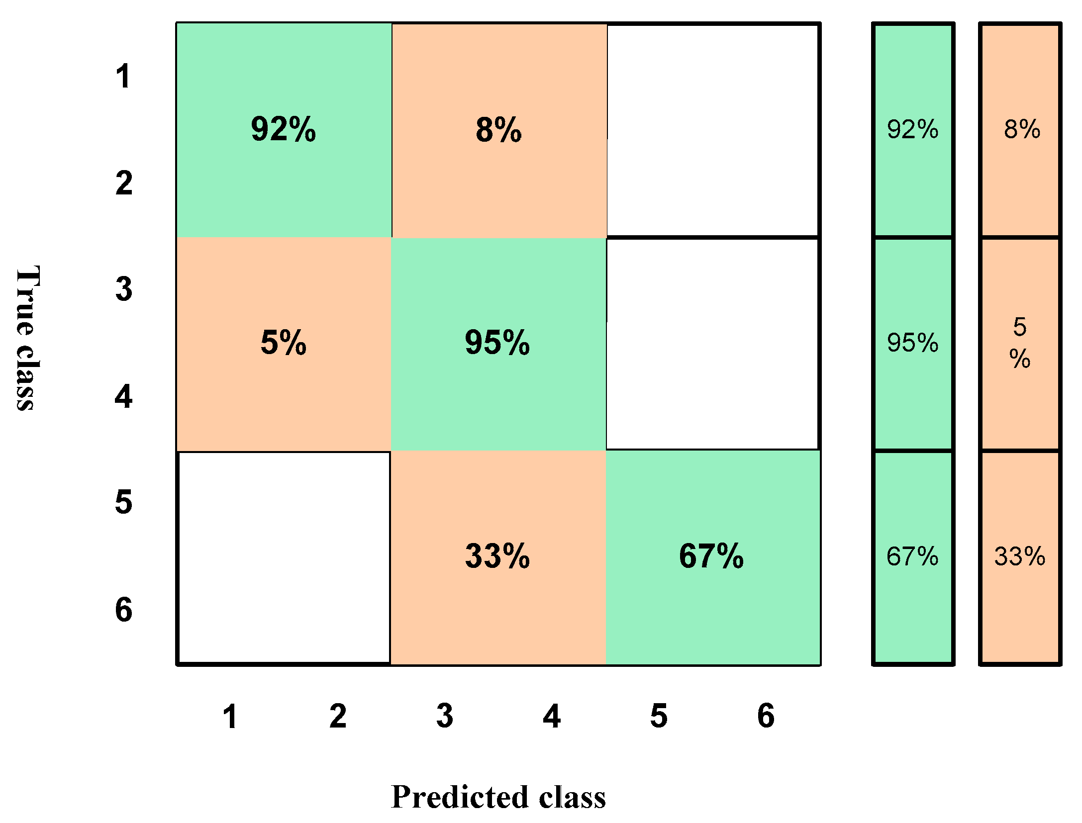
| 86.67 | |||||||||||||||||||
| Inputs Data | Actual WQI | Predicted WQI | ||||||||||||||||
|---|---|---|---|---|---|---|---|---|---|---|---|---|---|---|---|---|---|---|
| EC | PH | NTU | TDS | ALK. | TH | HCO3− | Cl− | SO42− | Ca2+ | Mg2+ | Na+ | K+ | NO3− | F− | Fe | As | Code | Prediction |
| 0.18 | 0.9 | 0.5 | 0.15 | 0.2 | 0.18 | 0.2 | 0.12 | 0.1 | 0.2 | 0.1 | 0.1 | 0.2 | 0.2 | 0.2 | 0.17 | 0 | 1 | 1 |
| 0.18 | 1 | 0.6 | 0.13 | 0.2 | 0.19 | 0.2 | 0.09 | 0.1 | 0.2 | 0.1 | 0.1 | 0.1 | 0.2 | 0.2 | 0.11 | 0.5 | 1 | 1 |
| 0.2 | 0.9 | 0.5 | 0.22 | 0.2 | 0.26 | 0.2 | 0.24 | 0.2 | 0.3 | 0.1 | 0.2 | 0.1 | 0.3 | 0.4 | 0.14 | 0 | 2 | 2 |
| 0.23 | 0.9 | 0.3 | 0.2 | 0.2 | 0.25 | 0.2 | 0.18 | 0.2 | 0.2 | 0.1 | 0.1 | 0.1 | 0.2 | 0.4 | 0.17 | 0.5 | 2 | 2 |
| 0.27 | 0.8 | 0.8 | 0.22 | 0.2 | 0.25 | 0.2 | 0.23 | 0.2 | 0.2 | 0.1 | 0.1 | 0.1 | 0.3 | 0.3 | 0.14 | 0.5 | 2 | 2 |
| 0.35 | 0.8 | 0.5 | 0.27 | 0.4 | 0.34 | 0.4 | 0.22 | 0.2 | 0.3 | 0.2 | 0.2 | 0.1 | 0.3 | 0.3 | 0.09 | 0.5 | 2 | 2 |
| 0.24 | 0.9 | 0.8 | 0.35 | 0.4 | 0.41 | 0.4 | 0.33 | 0.2 | 0.4 | 0.2 | 0.3 | 0.3 | 0.3 | 0.3 | 1.23 | 0 | 2 | 2 |
| 0.34 | 0.9 | 0.8 | 0.24 | 0.4 | 0.27 | 0.3 | 0.24 | 0.2 | 0.3 | 0.1 | 0.2 | 0.2 | 0.3 | 0.3 | 0.17 | 0.5 | 2 | 2 |
| 0.25 | 0.9 | 0.6 | 0.34 | 0.4 | 0.43 | 0.4 | 0.3 | 0.3 | 0.4 | 0.2 | 0.2 | 0.3 | 0.2 | 0.3 | 0.14 | 1 | 2 | 2 |
| 0.24 | 0.9 | 0.8 | 0.25 | 0.3 | 0.31 | 0.3 | 0.28 | 0.2 | 0.3 | 0.2 | 0.2 | 0.2 | 0.2 | 0.1 | 0 | 0 | 2 | 2 |
| 0.2 | 0.8 | 0.9 | 0.23 | 0.2 | 0.32 | 0.3 | 0.21 | 0.2 | 0.2 | 0.2 | 0.1 | 0.5 | 0.3 | 0.2 | 0.09 | 0.5 | 2 | 2 |
| 0.16 | 0.9 | 0.6 | 0.24 | 0.2 | 0.24 | 0.2 | 0.17 | 0.2 | 0.2 | 0.1 | 0.2 | 0.1 | 0.2 | 0.2 | 0.09 | 0.5 | 2 | 2 |
| 0.16 | 0.9 | 0.3 | 0.2 | 0.1 | 0.13 | 0.1 | 0.16 | 0.2 | 0.1 | 0.1 | 0.1 | 0.1 | 0.3 | 0.2 | 0.06 | 0 | 2 | 1 |
| 0.65 | 0.9 | 0.7 | 0.44 | 0.5 | 0.62 | 0.6 | 0.52 | 0.4 | 0.8 | 0.3 | 0.5 | 0.2 | 0.9 | 0.3 | 0.09 | 0 | 3 | 3 |
| 0.27 | 0.9 | 0.8 | 0.55 | 0.1 | 0.7 | 0.7 | 0.67 | 0.5 | 0.3 | 0.3 | 0.6 | 0.2 | 0.2 | 0.6 | 0.63 | 0 | 3 | 3 |
| 93.33 | ||||||||||||||||||
Disclaimer/Publisher’s Note: The statements, opinions and data contained in all publications are solely those of the individual author(s) and contributor(s) and not of MDPI and/or the editor(s). MDPI and/or the editor(s) disclaim responsibility for any injury to people or property resulting from any ideas, methods, instructions or products referred to in the content. |
© 2023 by the authors. Licensee MDPI, Basel, Switzerland. This article is an open access article distributed under the terms and conditions of the Creative Commons Attribution (CC BY) license (https://creativecommons.org/licenses/by/4.0/).
Share and Cite
Hussein, E.E.; Jat Baloch, M.Y.; Nigar, A.; Abualkhair, H.F.; Aldawood, F.K.; Tageldin, E. Machine Learning Algorithms for Predicting the Water Quality Index. Water 2023, 15, 3540. https://doi.org/10.3390/w15203540
Hussein EE, Jat Baloch MY, Nigar A, Abualkhair HF, Aldawood FK, Tageldin E. Machine Learning Algorithms for Predicting the Water Quality Index. Water. 2023; 15(20):3540. https://doi.org/10.3390/w15203540
Chicago/Turabian StyleHussein, Enas E., Muhammad Yousuf Jat Baloch, Anam Nigar, Hussain F. Abualkhair, Faisal Khaled Aldawood, and Elsayed Tageldin. 2023. "Machine Learning Algorithms for Predicting the Water Quality Index" Water 15, no. 20: 3540. https://doi.org/10.3390/w15203540
APA StyleHussein, E. E., Jat Baloch, M. Y., Nigar, A., Abualkhair, H. F., Aldawood, F. K., & Tageldin, E. (2023). Machine Learning Algorithms for Predicting the Water Quality Index. Water, 15(20), 3540. https://doi.org/10.3390/w15203540